Multi-Response Optimization via Desirability Functionfor the Black Liquor DATA

Multi-Response Optimization via

Desirability Functionfor the Black

Liquor DATA

Anwar Fitrianto1,2,3,*, Habshah Midi1,2

1_{Department of Mathematics,}

2_{Institute for Mathematical Research, Universiti Putra Malaysia,} 43400 UPM Serdang, Selangor Darul Ehsan, Malaysia.

3_{Department of Statistics, Bogor Agricultural University of Indonesia}

*_{Corresponding email: [email protected]}

Abstract

The experiment that was conducted to examine the advanced oxidation of the black liquor effluent obtained from the pulp and paper industry using the dark Fenton reaction in a lab-scale experiment based on Central Composite Design. The three factors along with their range values in that experiment were temperature (298; 333, K), H2O2 concentration (29.4; 58.8, mM), and Fe(II) concentration (0.36; 8.95, mM). The range of the factors were examine at fixed phase pH=3. Three response variables studied in the experiment, namely, COD removal after 90 min(%), UV254 removal after 90 min(aromatic content,%), and UV280 removal after 90 min (lignin content, %). The most widespread application of the RSM is in the situation where input variables potentially influence some quality characteristics of a process. Due to the fact that the experiment has several response variables, we employed a desirability function approach to optimize the responses simultaneously at one best setting of available factors. The resulted simultaneous optimization of an experiment is, in fact, the real situation where the experimenter should deal with since in an experiment, there is certainly a single input setting. After analyzing the data, both separated for each response variable and simultaneous for all response variables provided the same terms (factors) which are significantly contribute to the quadratic model (H2O2 and Fe(II) concentration). Nevertheles, they produced different factor settings. Through desirability function approach, we found that the best settings are 46.84 mM and 6.771 mM of H2O2 and Fe(II) concentration, respectively. Those setting can be obtained at desirability function’s value of 0.782.

92 1. INTRODUCTION

Response Surface Methodology (RSM) is a collection of statistical and mathematicaltechniques useful for developing, improving, and optimizing processes ([1].The most widespread application of the RSM is in situation where input variables potentially influence some quality characteristics of a process.

Its origin was the work of Box and Wilson, [2]. It is used in many practical applications in which the goal is to identify the level of p design variables or factors



x x xp



x ₁, ₂,_, , that optimize a response, f

 

x , over an experimental region. Additionally, RSM is used to analyze and control the processes to obtain optimal condition and parameters [3]. The main objective of response surface method is to optimize the response in a process.

Most industrial processes and products have more than one response or quality characteristic which are called multiple-response surface (MRS). This factoften leads to involvedisproportionate and conflicting qualitycharacteristics (responses).Those responses must, in some sense, be optimized simultaneously to obtain the best levels of factors during process design. Optimal factor setting for one response may be far from optimal for another response. Multiple response optimizations allows for compromise among the various responses.

In an effort of obtaining simultaneous optimization steps, we will employ a black liquor dataset, which appeared in [4]. It is an investigation of the advanced oxidation of the black liquor effluent from the pulp and paper industry using the dark Fenton reaction in a lab-scale experiment. They used central composite (CCD) in the process.But, in this article, we focus the analysis on the procedures of doing simultaneous optimization since in [4], their focused is on individual response optimization.

2. REVIEWS OF MULTI-RESPONSE DEVELOPMENT IN RSM

Harrington, [6], presented an optimization schemeutilizing what he termed the desirability function. Meanwhile, [7] and [8] describedoptimization schemes based upon the linearprogramming model. However, a major disadvantageof these schemes is the philosophy upon whichthey are based. These methods involve optimizationof one response variable subject to constraints on the remaining response variables. [9] then gave a slight modificationof Harrington’s function.The dual response approach for two responses was given by Myers and Carter, [10].The responses were categorized as primary and secondary responses. In this approach, we need to identify the levels of the design variables that optimize a primary response which is depended on a secondary response that has been set to a particular value. The tworesponse functions are then combined into a single response function which is then optimized.

Thus far, the most commonly used approaches are desirability functions, [11], the generalized distance measure method by Khuri and Conlon, [12], and the weighted squared error loss methodby Vining, [13]. The desirability function method is one of the most popular for multiple response problems. In desirability function method, the response variable is transformed to give a desirability value which is proportional to the priority given to the response variable. In other words, this approach incorporates the priorities on the response function as a part of optimization by Osborne and Armocost, [14]. In this approach, multiple response functions are estimated as polynomial functionsof the factors or design variables.

2.1 Optimization in RSM

Let say we have a set of data containing observations on a response variable yand k controllable factors. The true value of the response variable can be expressed as:







 f x x x_k y ₁, ₂,_, ,

where is noise or error which is usually assumed to be distributed with mean zero and constant variance 2



 . The function f is a response surface model, usually unknown. One goal in experimental design is to fit a mathematical model as the function f. Knowledge of the form of the function, f, often found by fitting models to data obtained from designed experiments in order to provide a summary representation of the behavior of the response, as the predictor variables are changed. This might be done in order to optimize the response or to find what regions of the x -space lead to a desirable product, [15].

In a multiple responses experiment, suppose that each response variable can be expressed as:

 



i , m



y n

i x :R R 12,, ,

94

2.2 Desirability Function for Multi-Response Optimization

One useful approach to optimization of multiple responses is to utilize the simultaneousoptimization technique popularized by [11]. It is one of the most widely used methods in industry which is based on the idea that the "quality" of a product or process that has multiple quality characteristics, with one of them outside of some "desired" limits, is completely unacceptable. Their proceduremakes use of desirability functions. The common approach is to first transform each response y_i into an individual desirability function d_i

 

y_i that varies over the range0d_i

 

y_i 1_, where it takes a range of between 0 and 1, and increases as the correspondingresponse value becomes more desirable [16].

Depending on whether a particular response y_iis to be maximized, minimized, or assigned to a target value, different desirability functions di

 

yi can be

used. The individual desirabilitydi

 

yi will be as follows:

Target is the best (TB), the objective ismin



ˆ_i

 

ˆ; _i



2

x y θ x T ,

 

 

 

_{ }

 

_{ }

 

                                 i i i i i r i i i i i i i r i i i i i i i i U y U y T U T U y T y L L T L y L y y d x x x x x x ˆ if 0 ˆ if ˆ ˆ if ˆ ˆ if 0 ˆ ₍₁₎

Smaller better (SB), the objective is

 

x

x ;

ˆ ˆ

miny_i θ , or

 

 

 

_{ }

 

                    i i i i i r i i i i i i i i U y U y T U T U y T y y d x x x x ˆ if 0 ˆ if ˆ ˆ if 1 ˆ (2)

Larger better LB), the objective is

 

x

x ;

ˆ ˆ

maxy_i θ ,

 

 

 

_{ }

 

                    i i i i i r i i i i i i i i T y T y L L T L y L y y d x x x x ˆ if 1 ˆ if ˆ ˆ if 0 ˆ

, (3)

values of y_i, while T is _i target values desired for ith response, where Li Ti Ui,

[17]. At this point, ris the parameters that determine the shape of d_i

 

yˆ_i . A value of 1



r means that the desirability function is linear, r1means that the desirability function is convex, more importance should be attached to close with the target value, and when the shape of the d_i

 

yˆ_i is concave when the value is0r1 which means less importance tobe attached. The individual desirabilities are then combined using the geometric mean, which gives the overall desirability D:

 

 

 





m

m m y

d y

d y d

D 1 ˆ1  2 ˆ2  ˆ 1 _,

Where m denotes the number of responses.

In fact, RSM normally starts with a series of steepest ascent/descent method based on a first-order model until a practicable higher-order model is suitable. For its simplicity, let assume here thatyhas been determined to be of second-order after steepest ascent method.

3. THE BLACK LIQUOR DATA

96

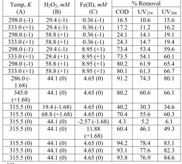
Table 1: Central composite design for Black Liquor data with the actual and coded values

Temp, K (A)

H2O2, mM (B)

Fe(II), mM (C)

% Removal COD UV254 UV280 298.0 (-1) 29.4 (-1) 0.36 (-1) 16.5 10.6 15.6 333.0 (+1) 29.4 (-1) 0.36 (-1) 17.2 11.2 16.2 298.0 (-1) 58.8 (+1) 0.36 (-1) 24.1 14.1 19.1 333.0 (+1) 58.8 (+1) 0.36 (-1) 24.3 14.7 19.4 298.0 (-1) 29.4 (-1) 8.95 (+1) 73.4 53.4 59.6 333.0 (+1) 29.4 (+1) 8.95 (+1) 73.5 54.1 60.1 298.0 (-1) 58.8 (+1) 8.95 (+1) 80.2 61.9 65.4 333.0 (+1) 58.8 (+1) 8.95 (+1) 80.1 61.3 66.7

286.0 (-1.68)

44.1 (0) 4.65 (0) 91.2 74.3 80.1

345.0

(+1.68) 44.1 (0) 4.65 (0) 80.2 60.6 66.1 315.5 (0) 19.4 (-1.68) 4.65 (0) 40.2 30.3 34.6 315.5 (0) 68.8 (+1.68) 4.65 (0) 70.4 55.6 60.3 315.5 (0) 44.1 (0) -2.57 (-1.68) 4.3 5.2 6.1 315.5 (0) 44.1 (0) 11.88

(+1.68)

60.4 46.1 49.3

315.5 (0) 44.1 (0) 4.65 (0) 94.2 78.4 83.1 315.5 (0) 44.1 (0) 4.65 (0) 93.1 77.6 82.3 315.5 (0) 44.1 (0) 4.65 (0) 93.8 76.9 84.6 Source :[4]

4. RESULTS AND DISCUSSION

4.1 Model Fitting for Individual Response Variable

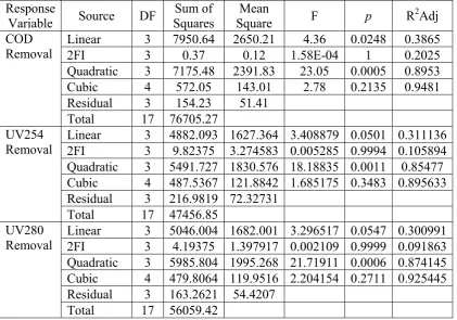
Table 2: Sequential model sum of squares and coefficient of determination of COD Removal, UV254 Removal, and UV280 Removal after 90 minutes (%) Response

Variable Source DF Squares Sum of Square Mean F p R2Adj COD

Removal

Linear 3 7950.64 2650.21 4.36 0.0248 0.3865

2FI 3 0.37 0.12 1.58E-04 1 0.2025

Quadratic 3 7175.48 2391.83 23.05 0.0005 0.8953

Cubic 4 572.05 143.01 2.78 0.2135 0.9481

Residual 3 154.23 51.41

Total 17 76705.27

UV254

Removal Linear 3 2FI 3 4882.093 1627.364 3.408879 0.0501 9.82375 3.274583 0.005285 0.9994 0.3111360.105894 Quadratic 3 5491.727 1830.576 18.18835 0.0011 0.85477 Cubic 4 487.5367 121.8842 1.685175 0.3483 0.895633

Residual 3 216.9819 72.32731

Total 17 47456.85

UV280

Removal Linear 3 2FI 3 5046.004 1682.001 3.296517 0.0547 4.19375 1.397917 0.002109 0.9999 0.3009910.091863 Quadratic 3 5985.804 1995.268 21.71911 0.0006 0.874145 Cubic 4 479.8064 119.9516 2.204154 0.2711 0.925445

Residual 3 163.2621 54.4207

Total 17 56059.42

Then we tried to fit the data with higher order model since, in general, first order model is not suitable, and we found that quadratic polynomial fits to all response variables with quite high value of adjusted R2.

Next step is then to find out terms in the suitable model for each response variable.A full quadratic response surface model with design variable inputs,x₁,x₂ and x₃with corresponding jth response variable y_jis formulated as follows:

 

 

   

        

 0 1x1 2x2 3x3 4x1x2 5x1x3 5x2x3 6x1x2x3

yj , (4)

where _i’s are polynomial regression coefficients of the input variables that were estimated by least squares fitting of the model to the experimental results obtained at the design points, and  is random errors. But since we found that the temperature (A, x₁) in all terms were not significant in the quadratic model, then we remove all

1

x related term from the Eq. (4).Curvature contribution was determined through

central composite design to obtain final reduced second-order model in the terms of

1

98

2 3 2

2 3

2 16.52 0.06 1.19

05 . 6 57 . 104

ˆ x x x x

y_COD     



_R2 _0.9188



2 3 2

2 3

2

254 97.31 5.43 13.63 0.06 1.01

ˆ x x x x

y_UV     



_R2 _0.87



2 3 2

2 3

2

280 94.63 5.52 14.28 0.06 1.07

ˆ x x x x

y_UV     



_R2 _0.8777



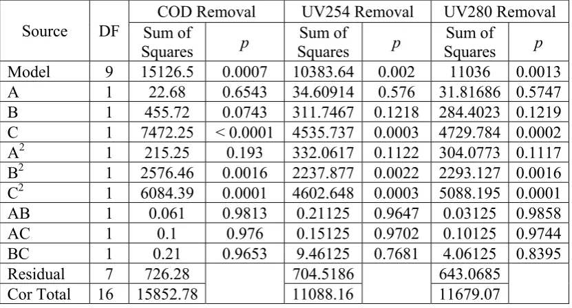
Table 3: Analysis of variance for response variables with full quadratic polynomial model

Source DF

COD Removal UV254 Removal UV280 Removal Sum of

Squares p Squares Sum of p Squares Sum of p Model 9 15126.5 0.0007 10383.64 0.002 11036 0.0013

A 1 22.68 0.6543 34.60914 0.576 31.81686 0.5747

B 1 455.72 0.0743 311.7467 0.1218 284.4023 0.1219

C 1 7472.25 < 0.0001 4535.737 0.0003 4729.784 0.0002 A2 1 215.25 0.193 332.0617 0.1122 304.0773 0.1117 B2 1 2576.46 0.0016 2237.877 0.0022 2293.127 0.0016 C2 1 6084.39 0.0001 4602.648 0.0003 5088.195 0.0001

AB 1 0.061 0.9813 0.21125 0.9647 0.03125 0.9858

AC 1 0.1 0.976 0.15125 0.9702 0.10125 0.9744

BC 1 0.21 0.9653 9.46125 0.7681 4.06125 0.8395

Residual 7 726.28 704.5186 643.0685

Cor Total 16 15852.78 11088.16 11679.07

4.2 Individual and Composite Desirability

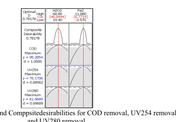
Figure 1: Individual and Comppsitedesirabilities for COD removal, UV254 removal, and UV280 removal.

In this study, there are three response variables on which the responses are competing with one another to determine the H2O2 and Fe(II) factor settings. The predicted maximum values of the responses are COD removal = 95.3854%, UV254 removal = 76.1706%, and UV280 removal = 81.9689% along with individual desirabilities of 1.0, 0.6856, and 0.6968, respectively (Figure 1). At the individual desirabilities, it has its own factor setting for each response variable which most probably have different factor setting. In fact, in a single experiment, it will have a single factor setting which is required to optimize all response variables.

The problem is solved through composite desirability. We obtained a value of composite desirability of D0.78178 to get a factors setting which optimize all response variables. The factors setting are 46.84 mMconcentration of H2O2and 6.771 mMconcentration of Fe(II).

5. CONCLUSIONS

100 REFERENCES

[1] Myers Raymond H., D.C. Montgomery, and M. Anderson-Cook. (2009). Response Surface Methodology: Process and Product Optimization using Designed Experiment, John Wiley & Sons. Hoboken, New Jersey.

[2] Box G.E.P. and Wilson, K.B. (1951). On the Experimental Attainment of Optimum Conditions.Journal of the Royal Statistical Society ,13, 1-45.

[3] Dehghani, K., Nekahi, A. (2010). Using Response Surface Methodology to Model the Age Hardening of AA6061, Metallurgical and Materials

Transaction A. 41A:3228 – 3237.

[4] Torrades, F., Samuel, S., Garcia-Hortal, J. A. (2011). Using Central

Composite Experimental Design to optimize the degradation of black liquor by Fenton Reagent, Desalination. 268: 97-102

[5] Hoerl, A.E.,(1959). Optimum Solution of Many Variables

Equations.Chemical Engineering Progress, vol.55, No.11, pp. 69–78.

[6] Harrington, E. C. Jr. (1965). The Desirability Function. Industrial Quality Control, Vol. 21, No. 10, pp. 494-498.

[7] Hartmann, N.E. and Beaumont, R. A. (1968). Optimum Compounding by Computer, Journal of the Institute of the Rubber Industry, Vol. 2, No. 6, pp. 272-275.

[8] Nicholson, T. A. J. and Pulle, R. D. (1969). Statistical and Optimization Techniques in the Design of Rubber Compounds, Computer Aided Design, Vol. 1, No. 1, pp.39-47.

[9] Gatza, P. E. and Mcmillan, R. C. (1972). The Use of Experimental Design and Computerized Data Analysis in Elastomer Development Studies, Division of Rubber Chemistry,American Chemical Society Fall Meeting, Paper No.6, Cincinnati, Ohio, October 3-6.

[10] Myers, R.H., and Carter,W.H., Jr. (1973). Response Surface Techniques for DualResponse Systems.Technometrics, Vol. 15, No.2, pp. 301–317.

[12] Khuri, A. I. and Conlon, M. (1981). Simultaneous Optimization of Multiple Responses Represented by Polynomial Regression-Functions.Technometrics 23, pp. 363-375.

[13] Vining, G. G. (1998). A Compromise Approach to Multi-response Optimization.Journal of Quality Technology 30, pp. 309-313.

[14] Osborne, D.M. and Armocost, R.L.(1997). State of the Art in Multiple Response Surface Methodology, Proceedings of the IEEE/SMC Conference, Orlando, Fl., pp. 3833–3838.

[15] Lin, D. K. J and John, J. P. (2006). Statistical Inference for Response Optima. In: ResponseSurface Methodology and Related Topics, A. I. Khuri (Editor), World Scientific, Singapore.

[16] Fuller, D and Scherer W. (1999). The desirability function: underlying assumptions and application implications. IEEE International Conference on Systems, Man and Cybernetics, p. 4016-21.