The Implementation of Double Bootstrap Method in Structural
Equation Modeling
Nor Iza Anuar Razak1, Zamira Hasanah Zamzuri∗2, and Nur Riza Mohd Suradi3
1,2,3School of Mathematical Sciences, Faculty of Science and Technology, Universiti
Kebangsaan Malaysia, 43600, Bangi, Selangor, Malaysia.
∗Corresponding author: [email protected]
Accuracy and reliability are fiery issues in Structural Equation Modeling (SEM). The single bootstrap method was outstanding, but the double bootstrap method was overlooked. The aim of this paper is to propose the usage of double raw data bootstrap method in SEM (double BOOT SEM). Double BOOT SEM is an enhanced version of raw data bootstrap method in SEM (BOOT SEM), where we resample raw data with replacement from each of the bootstrap samples repeatedly for a number of times. The performance of double BOOT SEM, BOOT SEM and SEM are evaluated through several summary statistics and confidence intervals. Results indicate that the performance of double BOOT SEM is more efficient compared to BOOT SEM and SEM in terms of smaller summary statistics values and narrowed bootstrap intervals.
Keywords: accuracy, confidence intervals, double bootstrap, Structural equation modeling.
I.
Introduction
Missing data remain a thorny issue in Struc-tural Equation Modeling (SEM), but the ac-curacy and reliability of SEM are no excep-tion. In spite of debate over accuracy and re-liability in SEM, research about it has con-tinued (Bentler, 2010, Boucard et al., 2007, Cheung and Lau, 2017, Hox and Maas, 2001, Lai and Kelley, 2011, Yang and Green, 2010). Commonly in accuracy and reliability issues, small sample sizes always lingering around as one of the factors contributed (Chumney, 2013, Ievers-Landis et al., 2011, Jung, 2013, Krebs-bach, 2014).
As the sample size decreases and non nor-mality increases, the increasing part of SEM analyses is incapable to converge (improper result may be found) (Kline, 2015). In the same way for small samples, maximum like-lihood and generalized least squares estima-tors tend to produce slightly inflated χ2 val-ues, even though multivariate normality ex-ists (Ievers-Landis et al., 2011). Significantly,
one can use a bootstrap method to treat small sample sizes and/or multivariate non normal data (Byrne, 2001, Ievers-Landis et al., 2011, Krebsbach, 2014). Also, the bootstrap method is used to assess the statistical accuracy and improve the performance of the model (Choi et al., 2015, Fitrianto and Midi, 2010, Lola and Zainuddin, 2016, Roberts and Martin, 2009).
Not only the bootstrap method becomes a nat-ural enhancement to statistical parameter esti-mation, but also supplementary potential small sample concerns (Efron, 1979).
There is a vast amount of literature on the implementation of SEM and the boot-strap method. Several studies have been pub-lished on dissimilarity and comparison of sev-eral bootstrap performances through a well-designed simulation study (Bollen and Stine, 1990, Fitrianto and Midi, 2010, MacKinnon et al., 2002, Ory and Mokhtarian, 2010, Preacher and Selig, 2012, Sharma and Kim, 2013, Zhang and Savalei, 2016, Zhang and Wang, 2008). Several critical issues are being raised and tackled such as sample size, normal-ity, mediation effect, outliers, effect size, boot-strap performance, and confidence intervals.
The concept of bootstrapping in SEM was well covered by Ievers-Landis et al. (2011) and Streukens and Leroi-Werelds (2016). Also, several studies of the bootstrap method in other models were reported by Assaf and Ag-bola (2011), Kounetas and Papathanassopou-los (2013), Lola and Zainuddin (2016), Pascual et al. (2006) and Roberts and Martin (2009). Improving the bootstrap method were carried out by Davidson and MacKinnon (2007) and McCullough and Vinod (1998). Here, we elab-orated some former research of SEM with or without the bootstrap method.
Ory and Mokhtarian (2010) studied the im-pact of non-normality, sample size and esti-mation technique on goodness-of-fit measures in structural equation modeling. Four estima-tion methods are used a) maximum likelihood (ML), b) asymptotic distribution free (ADF), c) bootstrapping and d) Mplus method. Over-all, when sample sizes are small and/or the high multivariate kurtosis, these methods yielded different outcomes pattern.
Zhang and Wang (2008) have conducted a simulation study to evaluate and compare the performance of three methods; a) Nor-mal Approximation Method b) Bootstrapping Raw Data Method and c) Bootstrapping Er-ror Method on mediation effects. Several
fac-tors were simulated including sample size, ef-fect size, distribution of residual errors, cov-erage probability, power and confidence inter-vals. In short, the error bootstrap and raw data bootstrap methods each showed the ultimate different results on different factors.
Fitrianto and Midi (2010) proposed a Rescaled Studentized Residual Bootstrap using Least Squares (ReSRB) method. The ReSRB method works by resampling the residuals from the original data. The performance of ReSRB measured via bias and root of mean square er-ror (RMSE) performances. The performances of ReSRB is compared with Raw Residual Bootstrap (RRB), Studentized Residual strap (SRB) and Jackknifed Residual Boot-strap (JRB). To sum up, the performances of ReSRB is superior to the competing method, as the performance of the bootstrapped estimates was well boosted.
Streukens and Leroi-Werelds (2016) were practically guiding in details the procedure of extracting more information from the boot-strap output. Focusing on European manage-ment research, this paper covered numerous is-sues of bootstrap in SEM such as bootstrap-ping and partial least squares-SEM (PLS-SEM) utilization. Some reviews of applied bootstrap methods also included, which including a) di-rect effect, b) non-didi-rect effect, c) comparison coefficients and d) coefficients of determination (R2).
In the hospitality industry, the Data En-velopment Analysis (DEA) double bootstrap method was used to evaluate the technical effi-ciency among Australian hotels (Assaf and Ag-bola, 2011). This research aims to a) examine empirically the performance of Australian ho-tels and b) studies the main factors of the tech-nical efficiency of hotels in Australia. A com-bination of two outputs and six inputs data set were used. As a result, the DEA double boot-strap model fixes the bias in the estimation of technical efficiency, compared to the traditional DEA model.
av-eraging for time series studies. The simula-tion study was run on four methods; dou-ble BOOT, BOOT, Bayesian model averaging (BMA) and a standard Akaike’s information criterion (AIC). On the whole, double BOOT produced smaller root mean squared error (RMSE) compared to BOOT, BMA, and stan-dard AIC. The performance of double BOOT also is far better from BOOT and BMA due to smaller variance value of estimates.
Most studies tend to focus on the single boot-strap (also known as an ordinary bootboot-strap) method in SEM, but not on the double boot-strap method. As a matter of fact, the double bootstrap method has a greater convergence property and the double bootstrap confidence interval typically has a higher order of accu-racy (McCullough and Vinod, 1998). Chernick (2007) describes the double bootstrap as an ap-proach to boost the bootstrap bias correction of the superficial error rate of a linear discrim-inant law.
As have been elaborated above, there is a lavish amount of bootstrapping method being implemented in SEM, or on the other model undoubtedly, each with remarkable estimation and outstanding contributions. Despite this in-terest, no one to the best of our knowledge has used double raw data bootstrap method in SEM. Hence, this paper aims to propose the implementation of a double raw data bootstrap method in SEM by using a Monte Carlo simu-lation and a set of real data and assessing the performance of the suggested method.
Given this aim, this paper is structured as follows. Section 2 set out the details of the single and double raw data bootstrap method used in SEM. A detailed Monte Carlo simula-tion design is detailed in Secsimula-tion 3. Secsimula-tion 4 is an encore of this paper, discussing the re-sults of the simulation study and application on a real data set. The performance of the proposed method will be fully stressed in this special part. Lastly, our conclusions are drawn in the final section; which is Section 5
II.
Methodology
Let M represents a mediation variable (also known as a mediator), X is an independent variable and Y is a dependent variable. Sym-bols ofa0 and b0 represent the intercepts, a, b and c are the parameters, whereas eM and eY both are residuals. The Structural Equation Modeling (SEM) can be expressed as follows:
M =a0+aX+eM (1)
Y =b0+bM +cX+eY (2)
The double raw data bootstrap method will be implemented on paired raw dataX,M and Y. Note that, this method is an extended ver-sion of the single raw data bootstrap method by Zhang and Wang (2008). Also, bear in mind that all the single bootstrap estimations are ex-ecuted before estimating the double bootstrap. The first stage is to ‘shuffle’ or sample the original data set (M, X and Y) with replace-ment to obtain a single set of bootstrap sample, denote asMb,Xb,Yb. Estimate the parameters
ˆ
a0ˆa,bˆ0, ˆband ˆcby using ordinary least squares method and statistic of interest, ˆθbis estimated from this bootstrap sample. The first stage of resampling is repeated for a number of repe-titions. From this bootstrap samples, single bootstrap SEM is estimated, Mib = ˆa0 + ˆaXib and Yb
BOOT SEM and double BOOT SEM by using calculation formula in Table 1 and confidence intervals in Table 2.
A. Performance measures
For the purpose of performance measures, for each of the model (SEM, BOOT SEM and Dou-ble BOOT SEM), we focus on the Standard Er-ror (SE), Mean Square ErEr-ror (MSE) and Root Mean Square Error (RMSE) to measure the ef-ficiency of models and also on the bias to es-timate its accuracy. Coupled with that, we construct the 95% of normal and t-distribution confidence intervals (CIs), and width of CIs will be evaluated. Assessment of all reliabil-ity of models is verified over the generated data once the new sample data,N, are applied to the SEM, BOOT SEM and double BOOT SEM. Table 1 summarized the statistical in-dicators for the evaluation of the performance measures from Walther and Moore (2005), AL-Lami et al. (2017) and Choi et al. (2015).
Likewise, the construction of 95% standard normal and t-distribution confidence intervals for SEM, BOOT SEM, and double BOOT SEM are constructed from Table 2. For 95% stan-dard normal confidence interval, the lower CI is computed by this formula; ˆθ−1.96√s
n, and as for upper CI, the formula is ˆθ+1.96√s
n in which ˆ
θand √s
n each is the sample statistics estimate and standard error of sample statistics estimate of model (SEM-N, BOOT SEM-N and Double BOOT SEM-N). Also, the 1.96 value is the ap-proximate value of the 97.5 percentile point of the normal distribution. Lastly, the CI width can be derive from the upper CI minus with the lower CI.
Meanwhile, the lower t-distribution CIs is computed by this formula; t = ˆθ −1.96√s
n, and upper t-distribution CIs is represent by
t = ˆθ+ 1.96√s
n, in which t-distribution with
n−1 degrees of freedom is the sampling dis-tribution of the t-value when the samples com-prise of independent identically distributed ob-servations from a normally distributed popu-lation. Note that, for t-distribution CIs, the
sample statistics estimate of model (ˆθ) are rep-resenting three models; SEM-t, BOOT SEM-t and Double BOOT SEM-t.
III.
Simulation design
The R programming language used to run the statistical simulations. The data were simulated using Equations (1) and (2), with sample data of M, X and Y are generated randomly from Gaussian distribution, with a mean of zero and one of standard deviation, ∼ N(0,1), i = 1, . . . , n. The path coefficients are set as a=b= 0.39 and c= 0.35. The val-ues are motivated by the research of Preacher and Selig (2012). Four different sample sizes were generated N = 30, 50, 75 and 100, for each sample size, 50 different sets of data were simulated. This results in a 1(X) x 1(M) x 1(Y) x 4(N) x 50 (sets onN) design, by which produced a total of 200 different combinations. In this simulation study, for each of the com-binations run, we only focus on the SE, MSE, RMSE, the bias and also construction of 95% of normal and t-distribution confidence inter-vals (CIs). One thousand (B= 1000 bootstrap resamples) replication were run for each of the combinations. Number of bootstrap repetition is suggested by Efron and Tibshirani (1985) as the number of bootstrap repetition should be at least 1000 when constructing confidence in-tervals around ˆθ.
The assumptions about nature and data set properties used in this study are based on Hallgren (2013) simulation. Data are gener-ated by following the Ordinary Least Square (OLS) regression assumptions; random vari-ables are sampled from populations with nor-mal distributions, residual errors are nornor-mally distributed (mean is zero), and the residual errors are homoscedastic and serially uncorre-lated.
IV.
Results and Discussion
sim-Table 1: Summary statistics Statistical indicator Calculation formula
Standard Error √s n;s=
q Pn
i=1 ( ˆYi−µ)2
n−1 Mean Square Error n1Pn
i=1( ˆYi−Yi)2 Root Mean Square
Er-ror n1
q Pn
i=1( ˆYi−Yi)2
Bias n1Pn
i=1( ˆYi−Yi)
whereYiand ˆYidenotes the observed and the estimated model fori= 1,2, . . . , n, andnis the number
of samples.
Table 2: 95% standard normal and t-distribution CIs Standard normal bootstrap CIs t-distribution CIs
C.I= ˆθ±(Z(1−α/2)·SEˆ ) C.I= ˆθ±(t(1−n−1α/2)·SEˆ )
where ˆθ is the sample statistics estimate of SEM, BOOT SEM and double BOOT SEM. ˆSE is the standard error of sample statistics estimate and (1−α/2) is 95% critical value of the standard normal distribution and t-distribution.
ulation study in Subsection 4.1 and application on real data in Subsection 4.2.
A. Simulation study
The sets of (M, X, Y) data were randomly gen-erated in line with the traditional SEM, M =
a0 +aX +eM and Y = b0 +bM +cX +eY. The performance of the Double Bootstrap SEM is evaluated with its competing method, SEM and Bootstrap SEM through the SE, MSE, RMSE and the bias. The results for each model are presented in Table 3.
Remarkably that the summary statistics of Double BOOT SEM were always lower than the competing methods, BOOT SEM and tra-ditional SEM; for all sample sizes involved. For instance, when n = 30, the SE values are de-creasing from 0.098697→0.097062→0.00302, which from traditional SEM to Bootstrap SEM and lastly to Double BOOT SEM. Importantly, the same decreasing pattern occurred for MSE and RMSE values. For example, for n = 30, the MSE value for SEM is 1.10359, BOOT SEM is 1.071198 and Double BOOT SEM is 0.042189. Also for RMSE, like whenn=50, the RMSE values decrease from 1.043647 (SEM) to 1.029303 (BOOT SEM) to 0.14175 (Double BOOT SEM).
As well as the bias values, bias values de-cline when double bootstrap method was ap-plied onto the traditional SEM. As when n
= 75, bias value for Double BOOT SEM is 0.093188, compared to the BOOT SEM and traditional SEM each is 0.835252 and 0.841151. Worth noting, the same declining pattern also spotted in other sample sizes. Lower bias value is always favorable as it indicates a higher ac-curacy of models. The most striking result from the simulation study is that the rapid changes detected between double BOOT SEM and BOOT SEM, for all sample size generated. In short, for all four performance measures, Double BOOT SEM notably outperform than BOOT SEM and SEM, which indicate the ro-bustness of the proposed method.
Table 3: Average SE, MSE, RMSE and bias
n Model SE MSE RMSE Bias
30 SEM 0.098697 1.10359 1.040704 0.831949 BOOT SEM 0.097062 1.071198 1.016814 0.816881 Double BOOT SEM 0.00302 0.042189 0.173714 0.170045
50 SEM 0.07276 1.101301 1.043647 0.835322
BOOT SEM 0.072187 1.081449 1.029303 0.828087
Double BOOT SEM 0.0021 0.030232 0.14175 0.137206
75 SEM 0.05923 1.109048 1.049454 0.841151 BOOT SEM 0.058605 1.094747 1.039288 0.835252 Double BOOT SEM 0.001825 0.014444 0.098753 0.093188
100 SEM 0.048938 1.178374 1.082792 0.863396
BOOT SEM 0.048482 1.167457 1.075154 0.859487
Double BOOT SEM 0.001512 0.01125 0.093165 0.087164
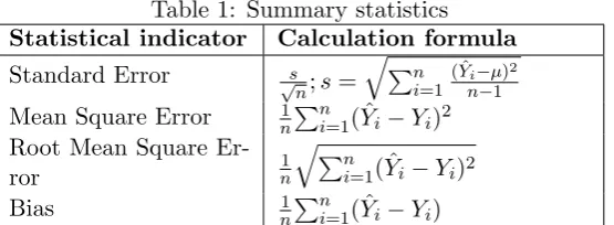
A narrow confidence interval is much more desirable than a wide one (Rumsey, 2007). Interestingly, the CI width for both Dou-ble BOOT N and DouDou-ble BOOT SEM-t remarkably narrower compared SEM-to SEM-the oSEM-ther model’s CIs, regarding for all sample sizes. For example, at 95% standard normal CIs, when n = 30, CI width for Double BOOT SEM-N is 0.011836, which narrower than the SEM-N and BOOT SEM-N, each with 0.386886 and 0.380474.
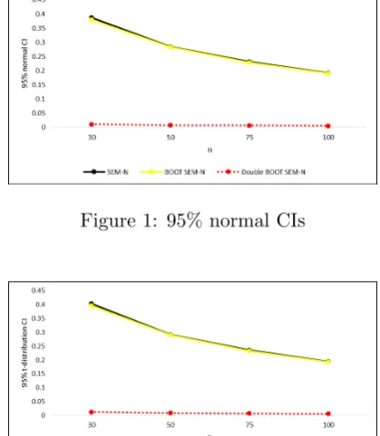
Besides, at 95% t-distribution CIs, whenn= 30, the CI width for Double BOOT SEM-t is 0.012351, while CI width for SEM-t and BOOT SEM-t are 0.403717 and 0.397026 each. The most remarkable result emerging from the t-distribution CIs result is that this result was in line with the standard normal CIs results. The CI width narrowed when the bootstrap method was applied to the traditional SEM.
Overall, for all the models involved, the CI width shows a consistent pattern, which is nar-rower as the sample size increase. Another key point is, CI width for double BOOT SEM is always remarkably showed the narrowest width compare to the other competing meth-ods, particularly between double BOOT SEM and BOOT SEM. The summary result from Ta-ble 4 is visualized in Graph 1 and Graph 2.
We have clearly shown that double Boot-strap SEM can offer more advantages over the
rival methods through the simulation study. Important to realize that the performance of double Bootstrap SEM are particularly no-ticeable compare to Bootstrap SEM. As sup-ported by Roberts and Martin (2009), the im-proved performance of double Bootstrap SEM is caused by a reduction in the variance of the estimates.
Figure 1: 95% normal CIs
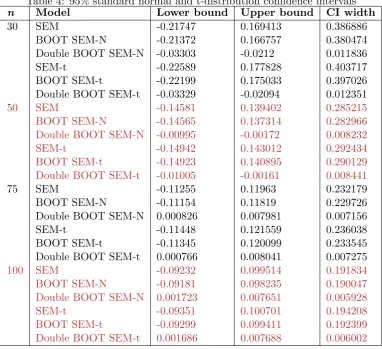
Table 4: 95% standard normal and t-distribution confidence intervals
n Model Lower bound Upper bound CI width
30 SEM -0.21747 0.169413 0.386886
BOOT SEM-N -0.21372 0.166757 0.380474 Double BOOT SEM-N -0.03303 -0.0212 0.011836
SEM-t -0.22589 0.177828 0.403717
BOOT SEM-t -0.22199 0.175033 0.397026 Double BOOT SEM-t -0.03329 -0.02094 0.012351
50 SEM -0.14581 0.139402 0.285215
BOOT SEM-N -0.14565 0.137314 0.282966
Double BOOT SEM-N -0.00995 -0.00172 0.008232
SEM-t -0.14942 0.143012 0.292434
BOOT SEM-t -0.14923 0.140895 0.290129
Double BOOT SEM-t -0.01005 -0.00161 0.008441
75 SEM -0.11255 0.11963 0.232179
BOOT SEM-N -0.11154 0.11819 0.229726 Double BOOT SEM-N 0.000826 0.007981 0.007156
SEM-t -0.11448 0.121559 0.236038
BOOT SEM-t -0.11345 0.120099 0.233545 Double BOOT SEM-t 0.000766 0.008041 0.007275
100 SEM -0.09232 0.099514 0.191834
BOOT SEM-N -0.09181 0.098235 0.190047
Double BOOT SEM-N 0.001723 0.007651 0.005928
SEM-t -0.09351 0.100701 0.194208
BOOT SEM-t -0.09299 0.099411 0.192399
Double BOOT SEM-t 0.001686 0.007688 0.006002
B. Application on real data
The same procedure of double raw data boot-strap method described in Section 2 was imple-mented to the real data. The secondary data set (24 samples) is obtained from the Institute of Marine Biology (IMB), Universiti Malaysia Terengganu. Data consists of three variables which consist of one treatment group of 100 mg/kg (seahorse extract), also known as food consumption and denoted as X variable. The mediator is the body weight, denoted as M
variable and diameter of lumen denoted as Y
variable.
These results indicate that the standard er-ror value for double BOOT SEM is 2.252811e-05, which much smaller than BOOT SEM and SEM, each with 2.841251e-04 and 4.915769e-04.Also, CIs width for Double BOOT SEM-N is 8.830858e-05, much narrower than BOOT
SEM-N and SEM-N, each with 1.113750e-03 and 1.926946e-1.113750e-03. The same pattern also occurred for Double BOOT SEM-t, the CIs width is 0.0000932059, way better than the SEM-t (0.0020338086) and BOOT-SEM-t (0.0011755153). Notably, the performance of the double raw data bootstrap method also works well on real data.
confi-dence intervals.
With attention to both simulation study and application on real data outcomes, positively, the double raw data bootstrap method works well and be able to offer advantages over sin-gle raw data bootstrap method or traditional method. While the performance of BOOT SEM is much better than SEM, the bizarrely noticeable performance is from double BOOT SEM. The double raw data bootstrap method in SEM can offer extra benefits in terms of smaller summary statistics and narrower confi-dence intervals.
V.
Conclusion
We have illustrated the implementation of dou-ble raw data bootstrap procedure in SEM. The analysis was performed by Monte Carlo simu-lation on X, M and Y set of raw data and a set of real data. Through the simulation study, the performance of double BOOT SEM, BOOT SEM and SEM are evaluated not only through the SE, MSE, RMSE, bias but also by con-structing confidence intervals. Formally, our simulation and implementation on real data re-sults directly showed that the performance of the proposed method, double raw data boot-strap method is more competent compared to the traditional SEM, in terms of smaller sum-mary statistics values and narrowed bootstrap intervals. In short, the double raw data boot-strap method does improve statistical efficiency measured. In essence, if improving the ac-curacy and reliability of the model is a con-cern, then double raw data bootstrap method in SEM (double BOOT SEM) offers a practical alternative to BOOT SEM and SEM.
Acknowledgements
The author would like to thank the Faculty of Science and Technology (FST), Universiti Kebangsaan Malaysia (UKM) for the grant FRGS/1/2015/ST06/UKM/02/1 and Mohd. Effendy, A.W. from UMT for the contribution of data.
References
[1] Alaa M AL-Lami, Ali M AL-Salihi, and Yaseen K AL-Timimi. Parameterization of the downward long wave radiation un-der clear-sky condition in baghdad, iraq. Sciences, 10(1):10–17, 2017.
[2] A Georges Assaf and Frank W Agbola. Modelling the performance of australian hotels: a dea double bootstrap approach. Tourism Economics, 17(1):73–89, 2011.
[3] Peter M Bentler. Sem with simplicity and accuracy. Journal of Consumer Psychol-ogy, 20(2):215–220, 2010.
[4] Kenneth A Bollen and Robert Stine. Di-rect and indiDi-rect effects: Classical and bootstrap estimates of variability. Socio-logical methodology, pages 115–140, 1990.
[5] Aur´elie Boucard, Alain Marchand, and Xavier Nogu`es. Reliability and validity of structural equation modeling applied to neuroimaging data: a simulation study. Journal of neuroscience methods, 166(2): 278–292, 2007.
[6] Barbara M Byrne. Structural equation modeling: Perspectives on the present and the future. International Journal of Testing, 1(3-4):327–334, 2001.
[7] MR Chernick. Bootstrap methods: A guide for researchers and practitioners, 2007.
[8] Gordon W Cheung and Rebecca S Lau. Accuracy of parameter estimates and confidence intervals in moderated media-tion models: A comparison of regression and latent moderated structural equa-tions. Organizational Research Methods, 20(4):746–769, 2017.
bootstrap adoption. Journal of Mechan-ical Science and Technology, 29(1):279– 289, 2015.
[10] Frances L Chumney. Structural equation models with small samples: A compara-tive study of four approaches. 2013.
[11] Russell Davidson and James G MacKin-non. Improving the reliability of strap tests with the fast double boot-strap. Computational Statistics & Data Analysis, 51(7):3259–3281, 2007.
[12] B. Efron. Bootstrap methods: An-other look at the jackknife. Ann. Statist., 7(1):1–26, 01 1979. doi: 10.1214/aos/1176344552. URL https://doi.org/10.1214/aos/1176344552.
[13] Bradley Efron and Robert Tibshirani. The bootstrap method for assessing sta-tistical accuracy. Behaviormetrika, 12 (17):1–35, 1985.
[14] Anwar Fitrianto and Habshah Midi. Es-timating bias and rmse of indirect effects using rescaled residual bootstrap in me-diation analysis. WSEAS Transaction on Mathematics, 9(6):397–406, 2010.
[15] Kevin A Hallgren. Conducting simula-tion studies in the r programming envi-ronment. Tutorials in quantitative meth-ods for psychology, 9(2):43, 2013.
[16] Joop J Hox and Cora JM Maas. The ac-curacy of multilevel structural equation modeling with pseudobalanced groups and small samples. Structural equation modeling, 8(2):157–174, 2001.
[17] Carolyn E Ievers-Landis, Christopher J Burant, and Rebecca Hazen. The concept of bootstrapping of structural equation models with smaller samples: An illus-tration using mealtime rituals in diabetes management. Journal of Developmental & Behavioral Pediatrics, 32(8):619–626, 2011.
[18] Sunho Jung. Structural equation mod-eling with small sample sizes using two-stage ridge least-squares estimation. Be-havior research methods, 45(1):75–81, 2013.
[19] Rex B Kline. Principles and practice of structural equation modeling. Guilford publications, 2015.
[20] Kostas Kounetas and Fotis Papathanas-sopoulos. How efficient are greek hospi-tals? a case study using a double boot-strap dea approach. The European Jour-nal of Health Economics, 14(6):979–994, 2013.
[21] Craig Michael Krebsbach. Bootstrapping with small samples in structural equation modeling: Goodness of fit and confidence intervals. 2014.
[22] Keke Lai and Ken Kelley. Accuracy in parameter estimation for targeted effects in structural equation modeling: Sample size planning for narrow confidence inter-vals. Psychological Methods, 16(2):127, 2011.
[23] Chondra M Lockwood and David P MacKinnon. Bootstrapping the standard error of the mediated effect. In Proceed-ings of the 23rd annual meeting of SAS Users Group International, pages 997– 1002. Citeseer, 1998.
[24] Muhamad Safiih Lola and Nurul Hila Zainuddin. The performance of double bootstrap method for large sampling se-quence. 6:805–813, 2016.
[25] David P MacKinnon, Chondra M Lock-wood, Jeanne M Hoffman, Stephen G West, and Virgil Sheets. A comparison of methods to test mediation and other intervening variable effects. Psychologi-cal methods, 7(1):83, 2002.
[27] David T Ory and Patricia L Mokhtarian. The impact of non-normality, sample size and estimation technique on goodness-of-fit measures in structural equation mod-eling: evidence from ten empirical models of travel behavior. Quality & Quantity, 44(3):427–445, 2010.
[28] Lorenzo Pascual, Juan Romo, and Esther Ruiz. Bootstrap prediction for returns and volatilities in garch models. Com-putational Statistics & Data Analysis, 50 (9):2293–2312, 2006.
[29] Kristopher J Preacher and James P Selig. Advantages of monte carlo confidence in-tervals for indirect effects. Communica-tion Methods and Measures, 6(2):77–98, 2012.
[30] Steven Roberts and Michael A Martin. Bootstrap-after-bootstrap model averag-ing for reducaverag-ing model uncertainty in model selection for air pollution mortal-ity studies. Environmental health per-spectives, 118(1):131–136, 2009.
[31] Deborah J Rumsey. Intermediate statis-tics for dummies. John Wiley & Sons, 2007.
[32] Pratyush N Sharma and Kevin H Kim. A comparison of pls and ml bootstrap-ping techniques in sem: A monte carlo study. InNew perspectives in partial least squares and related methods, pages 201– 208. Springer, 2013.
[33] Sandra Streukens and Sara Leroi-Werelds. Bootstrapping and pls-sem: A step-by-step guide to get more out of your bootstrap results. European Management Journal, 34(6):618–632, 2016.
[34] Bruno A Walther and Joslin L Moore. The concepts of bias, precision and ac-curacy, and their use in testing the per-formance of species richness estimators, with a literature review of estimator
performance. Ecography, 28(6):815–829, 2005.
[35] Yanyun Yang and Samuel B Green. A note on structural equation modeling es-timates of reliability.Structural Equation Modeling, 17(1):66–81, 2010.
[36] Xijuan Zhang and Victoria Savalei. Boot-strapping confidence intervals for fit indexes in structural equation model-ing. Structural Equation Modeling: A Multidisciplinary Journal, 23(3):392– 408, 2016.