81
Differential Evolution Biogeography Based Optimization for
Linear Phase Fir Low Pass Filter Design
Surekha Rani* Balwinder Singh Dhaliwal Sandeep Singh Gill Department of ECE , Guru Nanak Dev Engineering College, Ludhiana,Punjab, India
* E-mail of the corresponding author: [email protected]
Abstract
This paper presents an efficient way of designing Linear Phase Finite Impulse Response (FIR) Filter using hybrid Differential Evolution (DE) and Biogeography based optimization (BBO) algorithms. DE is a fast and robust evolutionary algorithm tool for global optimization. On the other hand, BBO uses migration operator to share information among solutions. FIR filter of order 20 is designed using fitness function that is based on minimization of maximum ripples in pass band and stop band of the filter response. The result obtained from Differential Evolution Biogeography Based Optimization (DEBBO) for the FIR low pass filter is good in convergence speed and solution quality in terms of pass band ripple, stop band ripple, transition width.
Keywords: DE, BBO, DEBBO, Convergence, FIR Filter.
1. Introduction
Digital filter is an important part of digital signal processing. They can be implemented in hardware or software and can process both real time and recorded signals. It serves basic two functions of signal separation and signal restoration. There are two types of digital filters, FIR & Infinite Impulse Response (IIR) filter (Litwin 2000). FIR filter is more attractive due to its simplicity and stability. Recently, the use of nature-inspired optimization algorithm for the design of FIR filter is explored. DE (Storn and Price 1997), Differential Evolution Particle Swarm Optimization (DEPSO) (Luitel and Venayagamoorthy 2008), Particle Swarm Optimization with Quantum Infusion (PSO-QI) (Luitel and Venaygamoorthy 2008) has been used for the computationally efficient FIR digital filter design.
In this paper hybrid differential evolution biogeography based optimization algorithm is used for the designing of FIR low pass filter of order 20. The rest of this paper is organized as follows: Section 2 briefly describes problem formulation; proposed approach is presented in detail in section 3. Results of FIR filter is presented with DE and DEBBO in section 4. The last section i.e. section 5, is devoted to conclusion.
2. Problem Formulation
Filter is used to pass certain band of frequencies and it attenuates undesired frequencies. This paper presents design of linear phase FIR low pass filter using DEBBO. Linear phase FIR low pass filter has a symmetry property, due to that half of the coefficients are calculated by the proposed algorithm and for other they are concatenated to reduce dimension of the problem (Mandal et al 2012) . Transfer function and difference equation for the FIR low pass filter (Luitel and Venaygamoorthy 2008) is given in equation (1) & (2) respectively.
H Z h n z n=0, 1, 2………N (1) where h (n) is called impulse response.
y( n)=h (0) x (n)+h (1) x(n-1)+…… h (N) x(n-N) (2) where N is order of the filter and N+1 is the number of coefficients of the FIR low pass filter.
In case of PM algorithm, the ratio of δp/δs is fixed. To improve the flexibility in the error fitness function to be minimized, the fitness function given in equation (3) is used in this proposed work. The cost function used in this paper is based on minimization of maximum ripples in pass band and stop band of the filter response that is defined by (Luitel and Venaygamoorthy 2008) and it is given below:
J = Max (׀ E(ω) ׀ - δp) + Max (׀ E(ω) ׀ - δs) (3) ω ≤ωp ω ≥ωs
Where δp and δs are ripples in pass band and stop band, ωp and ωs are pass band and stop band cut off frequencies.
In case of low pass FIR filter:
Hi (e jw) = 1 for 1 ≤w ≤ wc 0 otherwise (4) Where wc is the cut off frequency of the filter to be desired. Hi(e jw) is the frequency response of the ideal filter.
3. Proposed DEBBO Hybrid Algorithm
82
optimization techniques, the DE and BBO which are briefly described as below.
3.1 DE
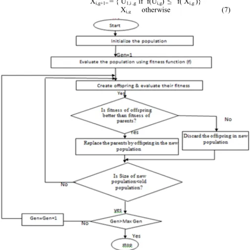
It is powerful population optimization technique that is used to create new candidate solution by the process of mutation and crossover (Storn and Price 1997). New candidate replaces the parents only if it has better fitness. The flow chart of DE is shown in Figure 1 and different steps of DE are explained below:
Initialization: Initially, the values associated with parameter vector are chosen randomly and it should cover the entire parameter space.
Mutation: This process begins with randomly selecting three individuals from generated population. Mutation strategy used in this work defined by (Storn and Price 1997) and it is given below (5) Where, i = 1,2 . . . , NP, where NP is the population size. r1, r2, r3 ϵ{1, . . . , NP} are randomly selected vectors from the population for mutation process and satisfy: r1 ≠ r2 ≠ r3 ≠ i. F ϵ [0, 1], F is the mutation control parameter.
Crossover: This process is used to generate the trial vector according to following rule (6). Ui,g= { v1,i,g if rand j <C r}
Xi,g Otherwise (6) Where j =1, 2, 3…..D, where D is dimension of the problem. Crossover rate, Cr ϵ [0, 1] and set by the user. Selection: The selection scheme of DE also differs from that of other Evolutionary Algorithms (EAs). The population for the next generation is selected from the individual in current population and its corresponding trial vector according to the following rule:
Xi,g+1= = { U1,i ,g if f(Ui,g) ≤ f( Xi,g )}
Xi,g otherwise (7)
FIGURE 1: Flow chart of DE algorithm
3.2. BBO
BBO (Simon 2008) is a relatively new population based biogeography inspired global optimization algorithm. In BBO, each individual is considered as ‘habitat’ with suitability index (HSI) which is similar to the fitness of EAs. Island with a high HSI means good solution whereas island with low HSI means poor solution. High HSI solution tends to share their features with low HSI solution. Low HSI solutions accept a lot of new features from high HSI solution.
83
lower value of λ corresponds to a good solution, whereas lower value of µ & higher value of λ corresponds to poor solution. The flow chart of BBO is given in Figure 2. Emigration rate λ k & immigration rate μ k for spices are given in (8), (9) respectively:
λ k I 1 k/n.) (8)
μ k E k/n (9) where I is maximum possible immigration rate, E is the maximum possible emigration rate. Maximum rate of
immigration and emigration is 1, n is the maximum number of species, k is kth number species.
FIGURE 2: Flow chart of BBO algorithm.
3.3. DEBBO for FIR Low Pass Filter
DEBBO technique used for the designing of FIR low pass filter used in this work is proposed in (Gong et al 2010). The flow chart of FIR low pass filter design using DEBBO is given in Figure 3 and the pseudo code for DEBBO is given in algorithm 1.
Algorithm 1:
Generate the initial population P
Evaluate the fitness for each individual in P while the halting criterion is not satisfied do
For each individual, map the fitness to the number of species
Calculate the immigration rate λi and the emigration rate µi for each individual Xi and modify the population for i = 1 to NP do
Select three vector randomly from population for mutation , r1≠ r2 ≠ r3≠ i ,where r1, r2, r3 three random population selected from population
jrand = randint(1,D) for j = 1 to D do if rand(0, 1) < λi then
if randj [0, 1) <CR or j = = jrand then U i (j) = Xr1 (j) + F × (Xr2 (j) − Xr3 (j))
84 else
Select Xk with probability α µ k U i (j) = X k(j) end if else U i (j) = X i(j) end if end for end for for i = 1 to NP do Evaluate the offspring Ui if Ui is better than Pi then Pi=Ui
end if end for end while
85
4. Results & Discussion
A linear phase FIR filter is designed in this work to find just half of the coefficients instead of all the coefficients. Phase linearity of the filter is guaranteed by assuming symmetry of the approximate filter which reduces the dimension of the problem by half. To design FIR low pass filter, the order of the filter is taken as 20, which ensure that length of the coefficients will be 21. Other specifications for the FIR low pass filter are taken as fs = 1Hz, No. of sampling points = 512, ωp = 0.45, ωs = 0.55, δp = 0.1, δs = 0.01, Transition width= 0.1.
4.1. Result of DE
For the above stated specifications, the filter is designed using DE algorithm. For the designing of FIR low pass filter using DE, some parameters of DE are to be selected. The Table 1 describes the different DE parameters.
Table 1: DE Parameters Parameters Value Population size 20 Dimension (D) 11 Mutation Factor (F) 0.5 Crossover Rate (CR) 0.9 No of Iteration 1000 Convergence Graph of DE
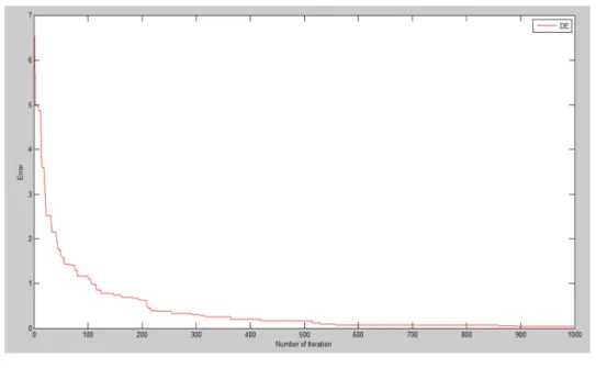
Convergence profile of optimization technique is defined as how fast function is converging to its minimum value. From Figure.4, it is cleared that it converges to its minimum value near 600 number of iteration with convergence error of 0.1341.
FIGURE 4: Convergence Graph for DE 4.2. Result of DEBBO
For the designing of FIR low pass filter using DEBBO, some parameters of DEBBO are to be selected. The Table 2 describes the different DEBBO parameters.
Table 2: DEBBO Parameters
Parameters Value Population size 20 Dimension (D) 11 Mutation Factor (F) 0.5 Crossover Rate (CR) 0.9 No of Iteration 1000
λ, µ Upper and lower bound range for λ and µ is [0,1]
86
Convergence Graph of DEBBO
Convergence profile of optimization technique is defined as how fast function is converging to its minimum value. From Figure.5, it is cleared that it converges to its minimum value near 200 number of iteration with convergence error of 0.0246. It is concluded from convergence graph of DE and DEBBO that DEBBO converge to its minimum value at less number of iteration than DE.
FIGURE 5: Convergence Graph for DEBBO
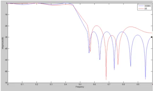
4.3. Comparison of Magnitude (dB) Plot of FIR Low Pass Filter of Order 20 using DE and DEBBO
Magnitude plot comparison of DE and DEBBO is shown in Figure 6 It is concluded that magnitude plot of DEBBO is much better in pass band ripple, stop band ripple and transition width than DE.
FIGURE 6: Comparison of Magnitude Plot of FIR Low Pass Filter of Order 20 using DE and DEBBO 4.4. Filter Coefficients Table of DE & DEBBO
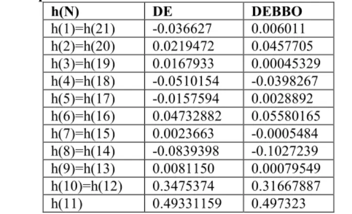
The FIR low pass filter of order 20 is designed using DE and DEBBO in this paper. No of coefficients is always 1 more than order of the filter. So for a filter with order 20 have 21 coefficients. Coefficients of the designed filters are given in Table 3.
87
Table 3: Optimized Coefficients of FIR Low Pass Filter of Order 20
h(N) DE DEBBO h(1)=h(21) -0.036627 0.006011 h(2)=h(20) 0.0219472 0.0457705 h(3)=h(19) 0.0167933 0.00045329 h(4)=h(18) -0.0510154 -0.0398267 h(5)=h(17) -0.0157594 0.0028892 h(6)=h(16) 0.04732882 0.05580165 h(7)=h(15) 0.0023663 -0.0005484 h(8)=h(14) -0.0839398 -0.1027239 h(9)=h(13) 0.0081150 0.00079549 h(10)=h(12) 0.3475374 0.31667887 h(11) 0.49331159 0.497323
4.5. Comparison of Proposed Result with Published Result
Table 3 shows comparison of different parameters of FIR low pass filter achieved by DEBBO and DE algorithms. Also these parameters are compared with PSO-QI (Luitel and Venaygamoorthy 2008) from literature with same input parameters. Maximum pass band ripple in case of DEBBO is 0.120, Transition width is 0.1177 and stop band ripple is 0.050. So From Table 4, it is clear that the proposed hybrid DEBBO algorithm has better performance than earlier used algorithm in terms pass band ripple, transition width and stop band attenuation. So the proposed algorithm results in better filter design which can be used in different applications.
Table 4: Comparison of Proposed Result with Published Result
Algorithm Maximum passband
ripple(Normalized)
Maximum stop Band Ripple (Normalized) Transition Width DE (Proposed work ) 0.1917 0.1026 0.1212 DEBBO (Proposed work ) 0.120 0.050 0.1177
PSO-QI (Luitel and
Venaygamoorthy 2008)
0.124 0.123 0.13
5. Conclusion
A low pass FIR filter of order 20 has been successfully designed using DEBBO hybrid algorithm. The convergence of DEBBO algorithm for this filter design is better than DE algorithm. The performance of the filter in terms of δ p, δ s and transition width is better than earlier published result of (Luitel and Venaygamoorthy 2008).
References
[1] Litwin, L.(2000) , “FIR and IIR Digital Filters”, IEEE Potentials, vol. 19, 4, pp. 28-31.
[2] Storn, R. and Price, K.(1997) “A Simple and Efficient Heuristic for Global Optimization over Continuous Spaces”, Journal of Global Optimization, vol. 11, 4, pp. 341–359.
[3] Luitel, B. and Venayagamoorthy, G. K.(2008), “Differential Evolution Particle Swarm Optimization for Digital Filter Computation”, Hong Kong, China, pp. 3954-3961.
[4] Luitel, B. and Venaygamoorthy,G.(2008), “Particle Swarm Optimization with Quantum Infusion for the Design of Digital Filters”, Proceedings of IEEE Swarm Intelligence Symposium, St. Louis, MO, pp. 1-8.
[5] Mandal, S. ,Ghoshal,S.K., Kar, R. and Mandal,D.(2012), “Design of Optimal Linear Phase FIR High Pass Filter Using Craziness Based Particle Swarm Optimization Technique”, Journal of King Saud University Computer and Information Sciences, vol. 24, pp. 83-92.
[6] Chattopadhyay,S. ,Sanyal,S.K. and Chandra,A.(2011), “Comparison of Various Mutation Schemes of Differential Evolution Algorithm for the Design of Low Pass FIR Filter”, International Conference on Sustainable Energy and Intelligent System, Tamil Nadu, India, pp. 809-814.
[7] Simon,D.(2008) “Biogeography-Based Optimization”, IEEE Transactions on Evolutionary Computation, vol. 12, 6, pp. 702-713.
[8] Gong,W., Cai, Z. and Ling,C.X.(2010), “Hybrid of Differential Evolution with Biogeography-Based Optimization for Global Numerical Optimization”, Soft Computing, vol. 15, 4, pp. 645-665.
88
AUTHOR PROFILE
Surekha--M.tech in Electronics and Communication Engineering from Guru Nanak Dev Engineering College,
Ludhiana. B.tech in Electronics and Communication Engineering from Beant College of Engineering and Technology, Gurdaspur, India. Areas of interest are Signal processing and Wireless.