Satisfactory optimization design for fractional order
PID controller
Tianyu Liua, Yuanjun Jiaa, Weidong Jina, Yong Wangb,∗
aDepartment of Automation, University of Science and Technology of China, Hefei 230022,
China
bCollege of Electrical Engineering, Southwest Jiaotong University, Chengdu 610031, China
Abstract
This paper presents a new parameters optimization approach for fractional or-der PID controllers, which uses a satisfactory optimization model. To fulfill different design performancespecificationsand constrains of systems, the appli-cation of multi-criterion satisfactory optimization to fractional control systems is considered. At the same time, the performance of fractional control systems controlled by fractional order controller and integer order controller is discussed. The simulation illustrates the effectiveness of the proposed method and the su-periority of the fractional order controller in both time domain and frequency domain.
Keywords: Satisfactory optimization, Multi-criterion satisfactory optimization, Fractional order system, Fractional order controller
1. Introduction
The key of optimization in a control system is to solve harmonious between constrains of system and performance specifications. The traditional optimiza-tion tries to satisfy optimizaoptimiza-tion targets under constrains. In order to obtain the optimal solution, it is necessary to findanaccurate mathematic model and
5
anideal objective function. Actually, due to lots of complex elements, the ac-tual control systems cannot meet it, even there is no optimal solution for some
∗Corresponding author
optimization problems. For this reason, satisfactory control and satisfactory optimization [1] is considered. Multi-criterion satisfactory optimization model is proposed by Jin et al. in [1]. Then it is employed in signal processing [1, 2],
10
computer network design [3] and fuzzy controller design [4].
In recent years, due to that many systems can be described accurately with the introduction of fractional order calculus, fractional order systems have at-tracted much attention in the engineering and physics fields, such as super-capacitor [5], human body circuit models [6]. Besides,fractional systems play
15
an increasingly important role in many scientific and engineering problems, such as fractional order system identification [7], stability analysis [8, 9], adaptive control [10, 11], signal processing [12, 13], etc.
The fractional order PID (FOPID) controller is the extension of the inte-ger order PID (IOPID) controller [14]. Comparedto the IOPID controller, the
20
FOPID has two more parameters: the integral orderλand the derivative order
µ. This make it more flexible. It can exert better robustness and accuracy for different controlled systems. It also can be used in industrial control [15, 16]. However, it is complicated to tune PID parameters. The performance specifica-tions in frequency domain, such as phase margin, gain crossover frequency and
25
robustness to variations in the gain of the plant, are often used to optimize the controller parameters in [16–19]. However, those methods are frequency-based methods. In practice, those methods guarantee good system frequency response but poor time domain response. Two sets of tuning rules for FOPID based on the first Ziegler-Nichols tuning rules are presented in [20]. However, this method
30
in [20] is only valid for those plants, whose step response is S-shaped.
Motivated by the above discussions, a novel method based on multi-criterion satisfactory optimization (MSO) is presented in this paper. The main contribu-tions are concluded as follows: a new fractional PID parameter tuning method is investigated. The MSO method is utilized to tuning controller parameters
35
for the first time. By selecting the appropriate performance specification and satisfactory rate function. This method can guarantee both good time domain performance and frequency domain performance. Several simulations verify
the effectiveness of this method. In this paper, a
The rest of this paper is organized as follows. Section 2 reviews the
fun-40
damental definitions of fractional order calculus and introduces the concept of the FOPID. A novel tuning method proposed for fractional order controllers (FOCs) based on multi-criterion satisfactory optimization model is described in Section 3. In Section 4, several numerical examples are provided. Finally, Section 5 draws some conclusions.
45
2. Preliminaries
The fractional order system is a mathematical model based on the fractional order differential equation. It is important to realize that the words ”fractional order systems” mean just ”systems which are better described by fractional order mathematical models [14].”
50
2.1. Fractional order calculus
Fractional order calculus means that the orders of the integral and derivative are arbitrary order. Fractional order calculus is an extension of the traditional integer ordercalculus . In this section, a brief summary of mathematical back-ground about fractional order calculus is introduced. More details can be found
55
in [21].
Generally, the fundamental operator of fractional order calculus can be de-fined as aD α tf(t) = dαf(t) dtα ,Re (α)>0, 1 ,Re (α) = 0, Rt af(τ) (dτ) −α ,Re (α)<0, (1)
wherea andt are the limits of the operation. αis the order of the integral or derivative, which can be real or complex.
60
The definitions of fractional order calculus given by different mathematicians are also different. The most popular definitions of fractional order calculus
mainly have the Riemann–Liouville (R–L) definition, the Gr¨unwald–Letnikov (G–L) definition and the Caputo definition, etc.
The Riemann–Liouville derivative definition of the orderαcan be given by
65 R aD α tf(t) = 1 Γ(m−a) d dt mZ t a f(τ) (t−τ)α−m+1dτ, (2) wherem−1< α < m,m∈N+, Γ(x) =R∞ 0 e
−ttx−1dtis the Gamma function. The Gr¨unwald–Letnikov definition can be written as
G aDtαf(t) = lim h→0 1 hα bt−a h c X j=0 (−1)j α j f(t−jh), (3)
wherehis the sample time,b·c is the flooring function. The Caputo derivative definition can be described as
C aD α tf(t) = 1 Γ(m−α) Z t a f(m)(τ) (t−τ)α−m+1dτ, (4) wherem−1< α < m,m∈N+. 70
Actually the fractional order definitions have no influence on this paper, so those can be abbreviated as aDα
t uniformly. For convenience, the Laplace transform also can be used to solve the differential equation. If we defineF(s) as the Laplace transform of the functionf(t), F(s) ≡ L[f(t)]. Consider the zero initial conditions, the Laplace transform of fractional order calculus is
75
L[Dαf(x)] =sαF(s), (5) whereDαrepresents theαth derivative off(t) from start point 0 tot.
2.2. Fractional order PID controllers
The differential equation of the FOPID controller is given(See [14])
u(t) =Kpe(t) +KiD−λe(t) +KdDµe(t), (6) whose transfer function can be written as
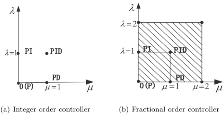
As is shown in Fig. 1, for the IOPID controller, the range of orders is limited
80
to four discrete points, corresponding to the P, PI, PD and PID four control model. The FOPID controller extends the four points to the plane defined by selecting the values of 0< λ, µ <2. This makes it more flexible. It can exert better robustness and accuracy for different controlled systems.
3, 3' 3,' 1 l= 1 m = 3
l
m
(a) Integer order controller3, 3' 3,'
m
2 l= 3 1 l= 1 m= m=2l
(b) Fractional order controller
Fig. 1. Range of control points of PID controllers with fractional order and integer order
3. Satisfactory optimization method
85
3.1. Multi-criterion satisfactory optimization model
In this subsection, the multi-criterion satisfactory optimization model [1], will be introduced .
Suppose the number of parameter variables in the optimization problem is
n. LetX be the parameter variable set. Then
90
X={(x1, x2, . . . , xn)|xi∈R, i= 1,2, . . . , n}, (8)
whereX ∈Rn.
Assumemis the number of the performance specifications to evaluate system performance,Qis the set of the system performance specifications, we have
In the feasible solution space of the closed-loop system, choose a vector of arbitrary feasible solution denoted asxj = [xj1, xj2, . . . , xjn]. Denote the vector
95
of system performance specification as qj = [qj1, q2j, . . . , qjm], where q j k is the performance value of thekth performance specificationqk respect to the system feasible solutionxj. In general, in the actual system the value of performance specification is related to more than one parameter variable. Thus, we have
qk =ϕ(x), such that
100
q= [q1, q2, . . . , qm] = [ϕ1(x), ϕ2(x), . . . , ϕm(x)] =ϕ(x), (10)
wherek= 1,2, . . . , m.
Letgk :R→[0,1] be the satisfactory rate function respect to qk, then the satisfactory rate ofqk can be described as
sk =gk(qk). (11)
Denotes= [s1, s2, . . . , sm] as the vector of satisfactory rate functions, where s∈[0,1]m. Then, we have
105
s=g(q) = [g1(q1), g2(q2), . . . , gm(qm)]. (12)
The synthesis satisfactory rate function is defined asf : [0,1]m→[0,1], then
sw=f(s) =f(s1, s2, . . . , sm), (13)
wheresw∈[0,1].
The value of system synthesis satisfactory function sw represents the syn-thesis satisfactory rate of this system to the designer under the feasible solution. In summary, based on the multi-criterion satisfactory optimization model, the optimization problem can be expressed as
max f(x)
s.t. gi(qi)∈[0,1], i = 1,2,3,· · ·,m,
(14)
wherex∈X⊆Rn,q∈Q⊆Rm.
3.2. Design of the FOPID controller
In this subsection, a new fractional PID parameter tuning method is in-vestigated. Using the aforementioned method, satisfactory optimization design for the FOPID controller is presented for the first time. The MSO method is mainly used to find the five parameters of the FOPID controller, such that the
115
controlled system obtains a satisfactory performance. The procedures to tune the FOPID are as follows:
step 1 Choosing the parameter variable set. For the FOPID controller, we choose five controller parameters Kp, Ki, Kd, λ and µ as parameter variable set, such that
120
X= [x1, x2, x3, x4, x5] = [Kp, Ki, Kd, λ, µ]. (15)
step 2 Choosing the performance specification set. In this study, three perfor-mance specifications in the time domain are concerned. The perforperfor-mance specification set includes overshootσ%, settling timets(2%) and rising timetr, such that
Q= [q1, q2, q3] = [σ%, ts, tr]. (16)
step 3 Selecting satisfactory rate function of each performance specification.
125
According to the selected performance specifications, the satisfactory rate functions are designed as
[s1, s2, s3] = [g1(σ%), g2(ts), g3(tr)]. (17)
step 4 Selecting synthesis satisfactory rate function. In general, the synthesis satisfactory rate function is defined as
sw= m
X
k=1
wksk. (18)
The weight reflects the importance of each performance specification, which
130
satisfyPm
Remark 1. This model provides a framework for parameter optimization, the specific parameter search algorithm can beselected by designer properly such as genetic algorithm, particle swarm optimization algorithm[22].
Remark 2. The satisfactory rate function reflects the tolerance of designer
135
to the variable range of the controller parameters. According to a satisfactory rate function, the optimal problem can be converted to a satisfactory optimiza-tion problem. It also influences the convergence of a algorithm[1].
4. Illustrative examples 4.1. Second-order plants
140
Consider a second-order plant (see [20]), whose transfer function is
G1(s) = 1
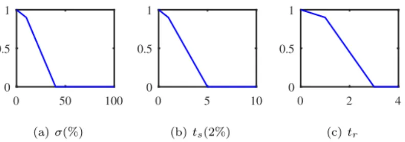
4.32s2+ 19.1801s+ 1. (19) Using the multi-criterion satisfactory optimization model to optimize the FOPID controller. The three satisfactory rate functions s1, s2 and s3 in this study are shown in Fig. 2. Take, for example, the overshootσ%, the explicit satisfactory rate function is as follow:
145 s1= 1 , q1≤0, 1−0.01q1 ,0< q1≤10, 1.2−0.03q1 ,10< q1≤40, 0 ,40< q1. (20)
For simplicity, each performance specification has the same weight. Thus we have sw= m X k=1 wksk, wm= 1 3, m= 3. (21)
Genetic algorithm is concerned to search satisfactory parameters. Set the population size M = 80, the evolution iteration G = 100, the crossover rate
Pc = 0.8, the mutation rate Pm = 0.05. Select the synthesis satisfactory rate
150
0 50 100 0 0.5 1 (a)σ(%) 0 5 10 0 0.5 1 (b)ts(2%) 0 2 4 0 0.5 1 (c)tr
Fig. 2. Satisfactory rate functions
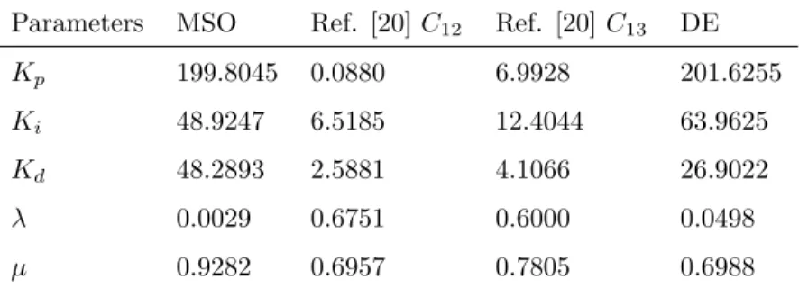
seconds. After 100 times iterations, the convergence of the synthesis satisfactory rate is shown in Fig. 3. Then the optimization parameters are shown in Table. 1. 0 20 40 60 80 100 0.3 0.4 0.5 0.6 0.7 0.8 0.9 1
synthesis satisfactory rate
Fig. 3. The convergence of the synthesis satisfactory rate
The corresponding FOPID can be designed as
155
C11(s) = 199.8045 +48.9247
s0.0029 + 48.2893s
0.9282. (22)
Literature [20] presents two sets of tuning rules for fractional PID. The two rules for tuning the parameters of fractional PIDs assumes the plant to have an S-shaped unit-step response. The first rule needs two tables of parameters, while the second, good for a narrower interval of values of L only, needs only
Table 1: FOPID controller parameters
Parameters MSO Ref. [20]C12 Ref. [20] C13 DE
Kp 199.8045 0.0880 6.9928 201.6255
Ki 48.9247 6.5185 12.4044 63.9625
Kd 48.2893 2.5881 4.1066 26.9022
λ 0.0029 0.6751 0.6000 0.0498
µ 0.9282 0.6957 0.7805 0.6988
one. Controllers obtained with the two sets of tuning rules [20] are
160 C12(s) = 0.0880 +6.5185 s0.6751 + 2.5881s 0.6957 , (23) C13(s) = 6.9928 +12.4044 s0.6000 + 4.1066s 0.7805. (24)
The controller obtained with differential evolution (DE) algorithm with pa-rameter self-adjusting [23] is
C14(s) = 201.6255 +63.9625
s0.0498 + 26.9022s
0.6988. (25)
In this work, the Oustaloup continuous approximation have been used to approximate fractional order operators to an integer transfer function. The
165
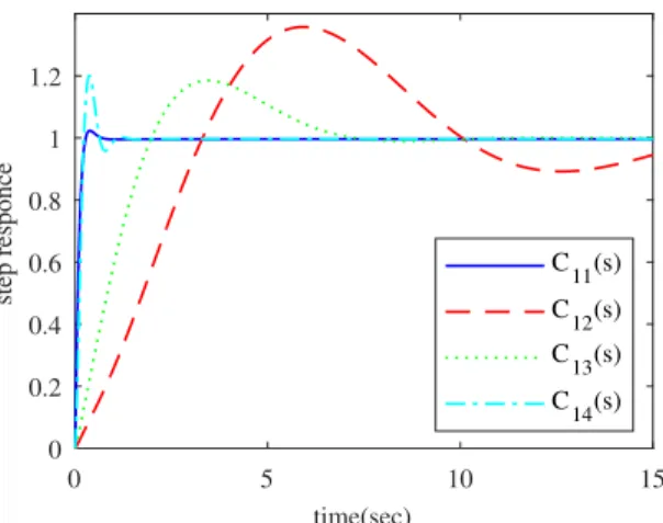
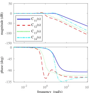
unit-step response, ISE and Bode diagrams of the controlled systemG1(s) with different FOCs are shown in Figs. 4, 5 and 6.
This comparison demonstrates that systems with a FOPID controller de-signed by the MSO method has smaller overshoot, faster response and larger phase margin. Using the proposed MSO method, the system performs faster
170
response in time domain and superiority in the frequency domain.
The specific performances of the controlled systemG1(s) with different con-trollers are shown in Table 2. Compare to other controllers, the controlled system with a controller designed by the MSO method performs a better per-formance in both time domain and frequency domain, the overall perper-formance
175
0 5 10 15 time(sec) 0 0.2 0.4 0.6 0.8 1 1.2 step responce C11(s) C 12(s) C13(s) C14(s)
Fig. 4. Step response of G1(s) controlled by different FOCs
0 5 10 15 time(sec) 0 20 40 60 80 100 120 140 160 180 ISE C11(s) C12(s) C13(s) C14(s)
-150 -100 -50 0 50 magnitude (dB) 10-2 100 102 104 -135 -90 -45 0 phase (deg) C 11(s) C12(s) C13(s) C14(s) frequency (rad/s)
Fig. 6. Bode diagrams of G1(s) controlled by different FOCs
of the proposed method in the parameter optimization design of the fractional order control system.
Table 2: Performance analysis of the controlled systemG1(s) under different controllers Controller σ(%) tr(s) ts(s) γ(◦) C11(s) 2.3209 0.2000 0.2200 122.5 C12(s) 35.8 3.303 15.87 69 C13(s) 18.6 1.982 6.889 99.7 C14(s) 8.5 0.327 1.471 71.5
4.2. Fractional order plants
Consider a fractional order plant [14], whose transfer function is
180
G2(s) =
1
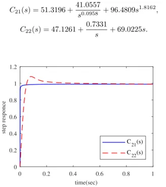
where the system nominal parameter values areα= 2.2 andβ = 0.9. The FOC and integer order controller (IOC) designed by the proposed method, respec-tively, are C21(s) = 51.3196 + 41.0557 s0.0958 + 96.4809s 1.8162, (27) C22(s) = 47.1261 +0.7331 s + 69.0225s. (28) 0 0.2 0.4 0.6 0.8 1 time(sec) 0 0.2 0.4 0.6 0.8 1 1.2 step responce C21(s) C 22(s)
Fig. 7. Step response ofG2(s) controlled by the FOC and the IOC
185 0 0.2 0.4 0.6 0.8 1 time(sec) 0 2 4 6 8 10 12 14 ISE C21(s) C22(s)
Fig. 8. ISE ofG2(s) controlled by the FOC and IOC
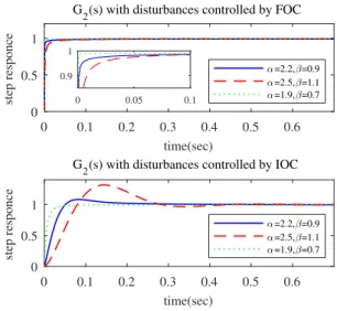
controllers are shown in Fig. 7. Due to the external environment conditions, true system parameters may change. Here, we assume that the disturbances occur in the parameters: α ∈ [1.9,2.5], β ∈ [0.7,1.1]. For the actual system, PID parameters are not the best match parameters. Using the aforementioned
190
controllers, the unit-step response of the disturbed system G2(s) is shown in
Fig. 9. Obviously, the performance specifications, such as overshoot, settling time and rising time, are slightly worse, but it still shows good robustness.
0 0.1 0.2 0.3 0.4 0.5 0.6 time(sec) 0 0.5 1 step responce
G2(s) with disturbances controlled by FOC
=2.2, =0.9 =2.5, =1.1 =1.9, =0.7 0 0.05 0.1 0.9 1 0 0.1 0.2 0.3 0.4 0.5 0.6 time(sec) 0 0.5 1 step responce G
2(s) with disturbances controlled by IOC
=2.2, =0.9 =2.5, =1.1 =1.9, =0.7
Fig. 9. Step response ofG2(s) with disturbances
For fractional order plants, comparing with the IOC, the closed-loop system with the FOC can obtain a better performance, even the disturbances occur in
195
the parameters. It is clear that the FOC can improve the system response by choosing the orders of the integral and derivative flexibly.
4.3. First-order plants with delay
Consider a first-order plant with delay [20], whose transfer function is
G3(s) = k 1 + 1.5se
−0.1s
Consider the nominal value ofk= 1, controllers obtained with first set of tuning
200
rules and second set of tuning rules [20], respectively, are
C31(s) = 0.6021 +0.6187 s1.3646 + 0.3105s 1.0618 , (30) C32(s) = 1.4098 +1.6486 s1.1011 −0.2139s 0.1855. (31)
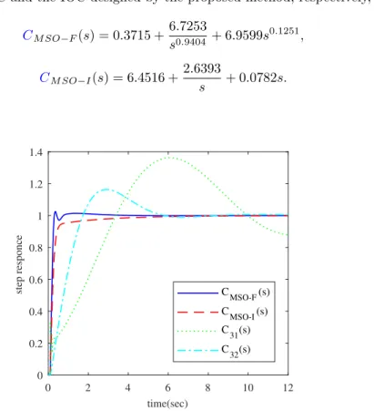
The FOC and the IOC designed by the proposed method, respectively, are
CM SO−F(s) = 0.3715 + 6.7253 s0.9404 + 6.9599s 0.1251, (32) CM SO−I(s) = 6.4516 + 2.6393 s + 0.0782s. (33) 0 2 4 6 8 10 12 time(sec) 0 0.2 0.4 0.6 0.8 1 1.2 1.4
step responce CMSO-F(s) CMSO-I(s) C31(s) C32(s)
Fig. 10. Step response of G2(s) controlled by different FOCs
205
The unit-step response of the controlled system G2(s) with different con-trollers, wherek= 1, is shown in Fig. 10.
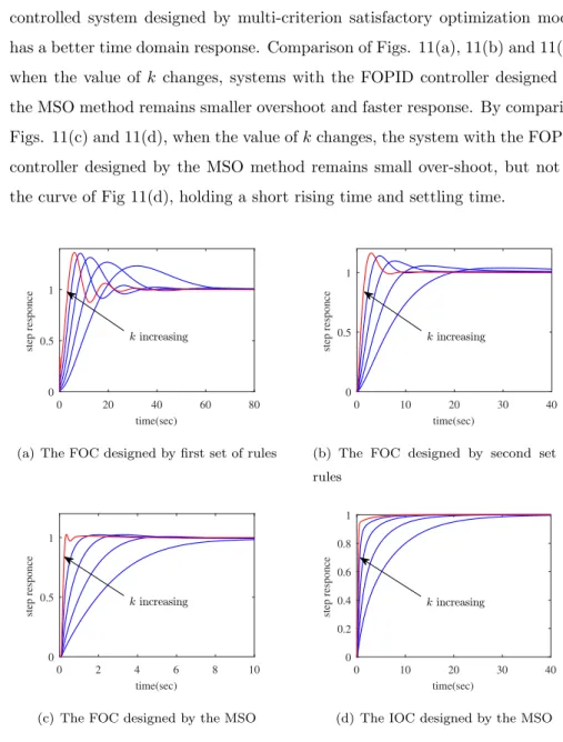
Assume the value ofkhas slightly changed, we set thek= 1,1/2,1/4,1/8,1/16 respectively. The unit-step response of systemG2(s) controlled by different con-trollers whenk changes is shown in Fig. 11.
As is shown in Fig. 11, compare to the IOC, the system with the FOC performs a better time domain response. Compared to other methods, the controlled system designed by multi-criterion satisfactory optimization model has a better time domain response. Comparison of Figs. 11(a), 11(b) and 11(c), when the value of k changes, systems with the FOPID controller designed by
215
the MSO method remains smaller overshoot and faster response. By comparing Figs. 11(c) and 11(d), when the value ofkchanges, the system with the FOPID controller designed by the MSO method remains small over-shoot, but not as the curve of Fig 11(d), holding a short rising time and settling time.
0 20 40 60 80 time(sec) 0 0.5 1 step responce
(a) The FOC designed by first set of rules
0 10 20 30 40 time(sec) 0 0.5 1 step responce
(b) The FOC designed by second set of rules 0 2 4 6 8 10 time(sec) 0 0.5 1 step responce
(c) The FOC designed by the MSO
0 10 20 30 40 time(sec) 0 0.2 0.4 0.6 0.8 1 step responce
(d) The IOC designed by the MSO
Fig. 11. Step response ofC2(s) controlled with PID controllers designed by different methods, whenkis 1, 1/2, 1/4, 1/8, 1/16.
In conclusion, compare to the IOPID controller, systems controlled by the
FOPID controller performs a faster and more accurate time domain response; compare to other methods, fractional order systems designed by the MSO method performs a faster and more accurate time domain response.
5. Conclusions
A novel method for the FOPID controller parameters setting is presented.
225
Contraposing the complexity of tuning the FOPID controller parameters, a new design guide based on multi-criterion satisfactory optimization model for the FOPID controller is proposed. The results demonstrate the effectiveness of the MSO method. Comparing with the conventional integer order PID controller, the proposed one can achieve a better performance in both time domain and
230
frequency domain.
Acknowledgments
The work described in this paper was fully supported by the National Nat-ural Science Foundation of China (No. 61573332, No. 61601431), the Fun-damental Research Funds for the Central Universities (No. WK2100100028),
235
the Anhui Provincial Natural Science Foundation (No. 1708085QF141) and the General Financial Grant from the China Postdoctoral Science Foundation (No. 2016M602032).
References
[1] W. Jin, D. Zhao, G. Li, The application of multi-criterion satisfactory
op-240
timization in FIR digital filter design, in: Proceedings of 2000 Internation-al Workshop on Autonomous DecentrInternation-alized Systems, 2000, pp. 227–230. doi:10.1109/IWADS.2000.880912.
[2] G. Zhang, W. Jin, F. Jin, Multi-criterion satisfactory optimization method for designing IIR digital filters, in: Proceedings of 2003 International
Conference on Communication Technology, 2003, pp. 1484–1490. doi: 10.1109/ICCT.2003.1209809.
[3] X. Tan, W. Jin, D. Zhao, The application of multi-criterion satisfactory optimization in computer networks design, in: Proceedings of the Fourth International Conference on Parallel and Distributed Computing,
Appli-250
cations and Technologies, 2003, pp. 660–664. doi:10.1109/PDCAT.2003. 1236386.
[4] D. Zhao, W. Jin, The application of multi-criterion satisfactory opti-mization in fuzzy controller design, in: The 2nd International Work-shop on Autonomous Decentralized Systems, 2002, pp. 162–167. doi:
255
10.1109/IWADS.2002.1194666.
[5] A. S. Elwakil, A. Allagui, B. J. Maundy, C. Psychalinos, A low frequency oscillator using a super-capacitor, International Journal of Electronics and Communications 70 (7) (2016) 970–973. doi:10.1016/j.aeue.2016.03. 020.
260
[6] V. D. Santis, V. Martynyuk, A. Lampasi, M. Fedula, M. Ortigueira, Fractional-order circuit models of the human body impedance for compli-ance tests against contact currents, International Journal of Electronics and Communications 78 (2017) 238–244. doi:10.1016/j.aeue.2017.04.035.
[7] Y. S. Hu, Y. Fan, Y. H. Wei, Y. Wang, Q. Liang, Subspace-based
265
continuous-time identification of fractional order systems from non-uniformly sampled data, International Journal of Systems Science 47 (1) (2016) 122–134. doi:10.1080/00207721.2015.1029568.
[8] Y. H. Wei, Y. Q. Chen, S. S. Cheng, Y. Wang, Completeness on the stability criterion of fractional order LTI systems, Fractional Calculus and Applied
270
Analysis 20 (1) (2017) 159–172. doi:10.1515/fca-2017-0008.
[9] J. G. Lu, Y. Q. Chen, Robust stability and stabilization of fractional-order interval systems with the fractional fractional-order α: The 0 < α < 1 case,
IEEE Transactions on Automatic Control 55 (1) (2010) 152–158. doi: 10.1109/TAC.2009.2033738.
275
[10] Y. Q. Chen, Y. H. Wei, S. Liang, Y. Wang, Indirect model reference adaptive control for a class of fractional order systems, Communication-s in Nonlinear Science and Numerical Simulation 39 (2016) 458–471. doi:10.1016/j.cnsns.2016.03.016.
[11] Y. H. Wei, P. W. Tse, Y. Zhao, Y. Wang, Adaptive backstepping output
280
feedback control for a class of nonlinear fractional order systems, Nonlinear Dynamics 86 (2) (2016) 1047–1056. doi:10.1007/s11071-016-2945-4.
[12] S. S. Cheng, Y. H. Wei, Y. Q. Chen, S. Liang, Y. Wang, A universal modi-fied LMS algorithm with iteration order hybrid switching, ISA Transactions 67 (2017) 67–75. doi:10.1016/j.isatra.2016.11.019.
285
[13] S. S. Cheng, Y. H. Wei, Y. Q. Chen, Y. Li, Y. Wang, An innovative frac-tional order LMS based on variable initial value and gradient order, Signal Processing 133 (2017) 260–269. doi:10.1016/j.sigpro.2016.11.026.
[14] I. Podlubny, Fractional-order systems and PIλDµ controllers, IEEE Trans-actions on Automatic Control 44 (1) (1999) 208–214. doi:10.1109/9.
290
739144.
[15] I. Dimeas, I. Petr´aˇs, C. Psychalinos, New analog implementation technique for fractional-order controller: a DC motor control, International Journal of Electronics and Communications 78 (2017) 192–200. doi:10.1016/j. aeue.2017.03.010.
295
[16] C. A. Monje, B. M. Vinagre, V. Feliu, Y. Q. Chen, Tuning and auto-tuning of fractional order controllers for industry applications, Control Engineering Practice 16 (7) (2008) 798–812. doi:10.1016/j.conengprac.2007.08. 006.
[17] H. S. Li, Y. Luo, Y. Q. Chen, A fractional order proportional and
deriva-300
Trans-actions on Control Systems Technology 18 (2) (2010) 516–520. doi: 10.1109/TCST.2009.2019120.
[18] C. A. Monje, B. M. Vinagre, Y. Q. Chen, V. Feliu, On fractional PIλ con-trollers: some tuning rules for robustness to plant uncertainties, Nonlinear
305
Dynamics 38 (1) (2004) 369–381. doi:10.1007/s11071-004-3767-3.
[19] D. Y. Xue, C. N. Zhao, Fractional order PID controller design for fractional order system, Control Theory and Applications 24 (5) (2007) 771–776. doi:10.3969/j.issn.1000-8152.2007.05.015.
[20] D. Val´erio, J. S. D. Costa, Tuning of fractional PID controllers with
Ziegler-310
Nichols-type rules, Signal Processing 86 (10) (2006) 2771–2784. doi:10. 1016/j.sigpro.2006.02.020.
[21] I. Podlubny, Fractional Differential Equations: an Introduction to Frac-tional Derivatives, FracFrac-tional Differential Equations, to Methods of Their Solution and Some of Their Applications, Academic Press, San Diego, 1999.
315
[22] M. Mitchell, An Introduction to Genetic Algorithms, MIT press, Mas-sachusetts, 1998.
[23] L. L. Huang, X. L. Zhou, J. H. Xiang, Self-adjusting design on parameters of the fractional order PID controller, Systems Engineering and Electronics 35 (5) (2013) 1064–1069. doi:10.3969/j.issn.1001-506X.2013.05.28.