Machine learning for image-based classification of Alzheimer's disease

Machine learning for image-based classification

of Alzheimer’s disease

Katherine Rachel Gray

A dissertation submitted in partial fulfilment of the requirements for the degree of Doctor of Philosophy

of

Imperial College London

October 3, 2012 Department of Computing

Declaration of originality

I declare that the work presented in this thesis is my own, unless specifically acknowledged.

Katherine R. Gray

Imaging biomarkers for Alzheimer’s disease are important for improved diagnosis and moni-toring, as well as drug discovery. Automated image-based classification of individual patients could provide valuable support for clinicians. This work investigates machine learning methods aimed at the early identification of Alzheimer’s disease, and prediction of progression in mild cognitive impairment. Data are obtained from the Alzheimer’s Disease Neuroimaging Initia-tive (ADNI) and the Australian Imaging, Biomarker and Lifestyle Flagship Study of Ageing (AIBL).

Multi-region analyses of cross-sectional and longitudinal FDG-PET images from ADNI are performed. Information extracted from FDG-PET images acquired at a single timepoint is used to achieve classification results comparable with those obtained using data from research-quality MRI, or cerebrospinal fluid biomarkers. The incorporation of longitudinal information results in improved classification performance.

Changes in multiple biomarkers may provide complementary information for the diagnosis and prognosis of Alzheimer’s disease. A multi-modality classification framework based on random forest-derived similarities is applied to imaging and biological data from ADNI. Random forests provide consistent similarities for multiple modalities, facilitating the combination of different types of features. Classification based on the combination of MRI volumes, FDG-PET in-tensities, cerebrospinal fluid biomarkers, and genetics out-performs classification based on any individual modality.

Multi-region analysis of MRI acquired at a single timepoint is used to show volumetric differ-ences in cognitively normal individuals differing in amyloid-based risk status for the develop-ment of Alzheimer’s disease. Reduced volumes in temporo-parietal and orbito-frontal regions in high-risk individuals from both ADNI and AIBL could be indicative of early signs of neurode-generation. This suggests that volumetric MRI can reveal structural brain changes preceding the onset of clinical symptoms.

Taken together, these results suggest that image-based classification can support diagnosis in Alzheimer’s disease and preceding stages. Future work may lead to more finely meshed prognostic data that may be useful clinically and for research.

Acknowledgements

I would first like to express my gratitude to both my supervisors, Daniel Rueckert and Alexander Hammers, for their enthusiasm and encouragement over the past few years.

I would also like to thank the many collaborators who have helped me along the way, in particular Rolf Heckemann, for providing motivation and invaluable advice, Paul Aljabar, for his mathematical assistance, Igor Yakushev, for kindly providing his reference cluster images, and Robin Wolz, for helping me get started. Thanks also to all members of the BioMedIA group, both past and present, for providing a great working environment.

I am grateful to the whole PredictAD team for their help during the brief time we were working together, and members of the Imperial Imaging Group, especially Jo Hajnal and Shiva Keiha-ninejad. I must also thank the EPSRC for financial support, and both the ADNI and AIBL investigators for providing the clinical and imaging data without which this research would not have been possible.

Finally, I am most grateful to my friends, especially everyone at Burles Farm, and, above all, my family and Jad for their support and encouragement throughout my studies.

Many thanks to you all!

1 Introduction 19

1.1 Alzheimer’s disease . . . 19

1.2 Neuroanatomy. . . 21

1.3 Neuropathology . . . 22

1.4 Neuroimaging . . . 24

1.4.1 Positron emission tomography . . . 24

1.4.2 Magnetic resonance imaging . . . 28

1.5 Biomarkers for Alzheimer’s disease . . . 32

1.5.1 Cerebrospinal fluid . . . 33

1.5.2 Magnetic resonance imaging . . . 34

1.5.3 Fluorodeoxyglucose positron emission tomography . . . 36

1.5.4 Pittsburgh compound B positron emission tomography . . . 37

1.6 Research contributions and thesis outline . . . 39

2 Background: PET and MR image analysis 41 2.1 Introduction . . . 41

CONTENTS 7 2.2 Image registration. . . 41 2.2.1 Transformation model . . . 42 2.2.2 Optimisation method . . . 50 2.2.3 Similarity metric . . . 50 2.2.4 Regularisation method . . . 53 2.2.5 Interpolation method . . . 53 2.3 Anatomical segmentation . . . 54 2.3.1 Manual segmentation . . . 54 2.3.2 Brain atlases . . . 55

2.3.3 Automated multi-atlas segmentation . . . 56

2.4 Statistical parametric mapping . . . 58

2.4.1 Image processing . . . 58

2.4.2 Statistical analyses . . . 59

2.4.3 Multiple comparison correction . . . 60

2.5 Conclusion . . . 61

3 Background: machine learning 62 3.1 Introduction . . . 62

3.2 Classification algorithms . . . 62

3.2.1 Linear discriminant functions . . . 63

3.2.2 Support vector machines . . . 65

3.2.4 Random forests . . . 71

3.3 Classifier performance . . . 74

3.3.1 Performance metrics . . . 74

3.3.2 Cross-validation . . . 76

3.4 Application to Alzheimer’s disease. . . 77

3.5 Conclusion . . . 79

4 Multi-region baseline FDG-PET for classification 80 4.1 Introduction . . . 80

4.2 Imaging data . . . 81

4.3 Image acquisition and pre-processing . . . 83

4.3.1 ADNI FDG-PET acquisition . . . 84

4.3.2 FDG-PET pre-processing . . . 85

4.3.3 ADNI MRI acquisition and pre-processing . . . 86

4.3.4 Co-registration of FDG-PET with MRI . . . 86

4.4 MRI anatomical segmentation . . . 87

4.4.1 Additional image processing . . . 88

4.4.2 Segmentation procedure . . . 89

4.4.3 Tissue class masking . . . 90

4.5 FDG-PET intensity normalisation . . . 91

4.5.1 Additional image processing . . . 91

CONTENTS 9

4.5.3 Reference cluster intensity normalisation . . . 95

4.6 Multi-region image analysis . . . 98

4.6.1 Region-based feature extraction . . . 99

4.6.2 Region-based group differences. . . 99

4.7 Classification experiments . . . 101

4.7.1 Methods . . . 101

4.7.2 Results. . . 103

4.7.3 Discussion . . . 104

4.8 Conclusion . . . 106

5 Multi-region longitudinal FDG-PET for classification 107 5.1 Introduction . . . 107

5.2 Imaging data . . . 109

5.3 Image acquisition and pre-processing . . . 110

5.4 Preliminary studies . . . 111 5.4.1 Hippocampal segmentation. . . 112 5.4.2 Image analysis. . . 113 5.4.3 Classification experiments . . . 114 5.4.4 Discussion . . . 116 5.5 Multi-region segmentation . . . 116

5.6 Multi-region image analysis . . . 118

5.7.1 Methods . . . 120

5.7.2 Results. . . 121

5.7.3 Discussion . . . 123

5.8 Conclusion . . . 125

6 Random forest-based similarities for multi-modality classification 126 6.1 Introduction . . . 126

6.2 Imaging and biological data . . . 128

6.2.1 Region-based MRI features. . . 128

6.2.2 Voxel-based FDG-PET features . . . 129

6.2.3 Biological CSF and ApoE genotype features . . . 129

6.3 Multi-modality classification framework . . . 130

6.4 Combining FDG-PET and MR imaging data . . . 131

6.4.1 Classification methodology . . . 131

6.4.2 Single-modality classification results. . . 132

6.4.3 Single-modality similarity-based classification results . . . 133

6.4.4 Multi-modality similarity-based classification results . . . 134

6.4.5 Discussion . . . 135

6.5 Combining imaging and biological data . . . 136

6.5.1 Classification methodology . . . 136

6.5.2 Single-modality classification results. . . 136

CONTENTS 11

6.5.4 Multi-modality similarity-based classification results . . . 139

6.5.5 Discussion . . . 140

6.6 Conclusion . . . 143

7 Early identification of Alzheimer’s disease 145 7.1 Introduction . . . 145

7.2 Imaging and biological data . . . 146

7.2.1 ADNI participants . . . 147

7.2.2 AIBL participants. . . 147

7.3 MRI acquisition and anatomical segmentation . . . 148

7.3.1 AIBL MRI acquisition . . . 148

7.3.2 AIBL MRI anatomical segmentation . . . 148

7.3.3 Computation of regional MRI volumes . . . 151

7.4 Amyloid-based risk status . . . 152

7.4.1 ADNI participants . . . 152

7.4.2 AIBL participants. . . 153

7.5 Volumetric differences between risk groups . . . 157

7.5.1 ADNI participants . . . 158

7.5.2 AIBL 1.5 T participants . . . 159

7.5.3 AIBL 3 T participants . . . 160

7.5.4 Discussion . . . 161

8 Overall conclusion 164

8.1 Contributions . . . 164

8.2 Future work . . . 166

9 Publications 168

Bibliography 171

A Hammers brain atlases 201

List of Tables

3.1 Confusion matrix for a binary classifier.. . . 74

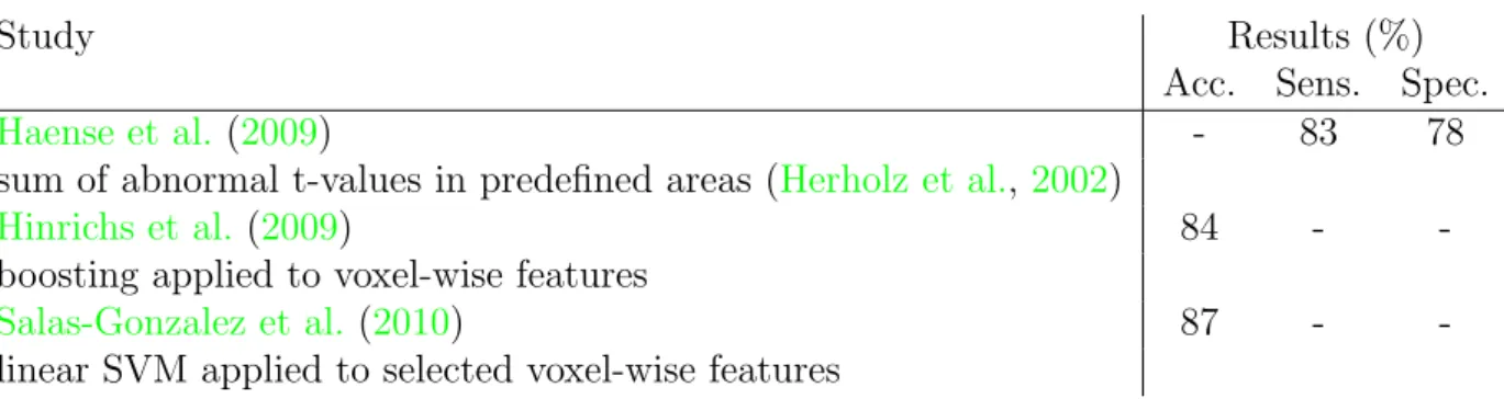
3.2 Summary of classification results based on cross-sectional ADNI FDG-PET data. 78 3.3 Summary of classification results based on MR imaging data. . . 79

4.1 Clinical and demographic information for the study population. . . 83

4.2 MAPER steps for aligning a single atlas MRI with the target MRI. . . 89

4.3 FWHM of the scanner-specific Gaussian smoothing kernels. . . 93

4.4 Classification results for SVM and Ada-LDA classifiers. . . 103

5.1 Clinical and demographic information for the study population. . . 109

5.2 Classification results based on longitudinal hippocampal FDG-PET. . . 115

5.3 Classification results based on longitudinal multi-region FDG-PET. . . 122

5.4 Classification results based on longitudinal multi-region FDG-PET after regression.123 6.1 Clinical and demographic information for participants with CSF data available. 128 6.2 Groupwise CSF measures and genetic information for the study population.. . . 130

6.3 Single-modality classification results based on the original data. . . 132

6.4 Single-modality classification results based on the embedded data. . . 134

6.5 Multi-modality classification results based on the jointly embedded data.. . . 134

6.6 Single-modality classification results based on the original data. . . 137

6.7 Single-modality classification results based on the embedded data. . . 139

6.8 Multi-modality classification results based on the jointly embedded data. . . 140

7.1 Clinical and demographic information for the study populations. . . 147

7.2 Details of the four PINCRAM iterations. . . 151

7.3 Regional volume differences between high- and low-risk sub-sets in ADNI.. . . . 158

7.4 Regional volume differences between high- and low-risk sub-sets in AIBL (1.5 T). 160 7.5 Regional volume differences between high- and low-risk sub-sets in AIBL (3 T). . 161

8.1 Comparison of key results from Chapters 4, 5 and 6.. . . 164

8.2 Summary of the ADNI studies. . . 166

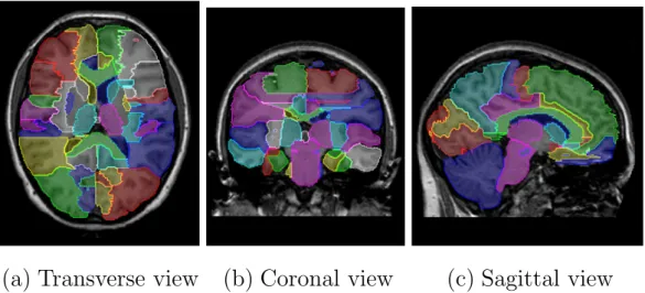
A.1 Anatomically defined regions manually delineated in the Hammers atlases. . . . 203

List of Figures

1.1 Illustrative timeline of AD progression. . . 20

1.2 Sagittal views of the brain, showing its gross anatomy. . . 21

1.3 Sagittal views of the ventricular system. . . 22

1.4 Axial views of the brain, showing the sub-structures of the medial temporal lobe. 22 1.5 Stages of PET image acquisition. . . 26

1.6 Image reconstruction by simple back projection. . . 27

1.7 Hydrogen atoms in the presence of a static magnetic field. . . 29

1.8 The application of Fourier transforms to MRI. . . 30

1.9 Example MRI pulse sequence. . . 31

1.10 Hypothetical temporal model of biomarker dynamics during AD progression. . . 33

1.11 MR images of healthy individuals and AD patients. . . 35

1.12 FDG-PET images of healthy individuals and AD patients. . . 36

1.13 PiB-PET images of healthy individuals and AD patients. . . 38

2.1 Illustration of possible rigid transformations. . . 43

2.2 Illustration of possible affine transformations. . . 45

2.3 Illustration of a nonrigid transformation. . . 47

2.4 Schematic sagittal brain view showing the anterior and posterior commissures. . 55

2.5 One of the manually delineated brain atlases used in this work.. . . 56

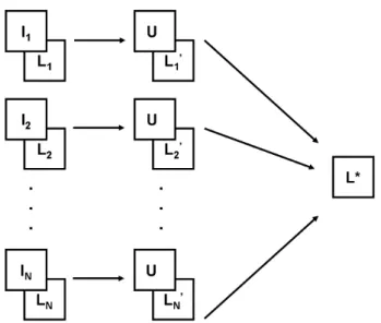
2.6 Schematic representation of the multi-atlas segmentation procedure. . . 57

2.7 Illustrative example of the SPM analysis procedure. . . 59

3.1 2-D illustration of the decision surface of a Fisher linear disciminant function. . 63

3.2 2-D illustration of the construction of a maximum-margin hyperplane. . . 65

3.3 A nonlinear boundary becomes a linear hyperplane in higher-dimensional space. 68 3.4 Illustration of the first two iterations in a typical boosting procedure. . . 70

3.5 Illustration of a random forest, showing two trees in detail. . . 71

3.6 Illustration of the ROC curve for a binary classifier. . . 76

4.1 Summary of exclusions. . . 83

4.2 Summary of FDG-PET and MRI acquisition and processing steps. . . 84

4.3 Number of baseline FDG-PET images acquired using each ADNI scanner model. 84 4.4 Illustration of the PET-MRI co-registration process. . . 87

4.5 Illustration of the brain masking process. . . 88

4.6 Illustration of the tissue classification results.. . . 89

4.7 Typical examples of a full and masked segmentation. . . 90

4.8 Typical examples showing alignment of MR and PET images to the MNI template. 92 4.9 Typical example images illustrating the FDG-PET smoothing process. . . 93

LIST OF FIGURES 17

4.10 Reduced FDG-PET intensity in AD versus HC using CGM normalisation. . . . 94

4.11 Reduced FDG-PET intensity in MCI versus HC using CGM normalisation. . . . 95

4.12 Increased FDG-PET intensity in AD and MCI versus HC. . . 96

4.13 Reduced FDG-PET intensity in AD versus HC using cluster normalisation. . . . 97

4.14 Reduced FDG-PET intensity in MCI versus HC using cluster normalisation. . . 97

4.15 Typical examples of the images required for regional FDG-PET feature extraction. 99 4.16 Group differences in the hippocampus and middle and inferior temporal gyri. . . 100

4.17 Regional t-values between AD patients and HC, and MCI patients and HC. . . . 100

5.1 Summary of exclusions. . . 109

5.2 Summary of the FDG-PET and MR image acquisition and pre-processing steps. 110 5.3 Alignment to baseline MRI space of 12-month MRI and FDG-PET images. . . . 112

5.4 Typical examples of the hippocampal segmentations. . . 113

5.5 Group differences in the hippocampus. . . 114

5.6 Propagation of the intracranial brain mask.. . . 117

5.7 Typical examples of masked multi-region segmentations. . . 117

5.8 Regional t-values based on cross-sectional and longitudinal FDG-PET features. . 119

5.9 Classification accuracies based on the five feature sets studied. . . 121

5.10 ROC curves for the best performing combined feature. . . 122

6.1 Schematic overview of the proposed multi-modality classification approach. . . . 130

6.3 Feature importances for distinguishing between clinical groups. . . 137

6.4 Similarity matrices for all three group pairs based on the four modalities. . . 138

6.5 Cobweb plots showing the distribution of parameters selected for classification. . 140

7.1 Illustration of the bias correction procedure. . . 149

7.2 Schematic representation of a single PINCRAM iteration. . . 150

7.3 Illustration of the PINCRAM procedure. . . 151

7.4 Summary of the ADNI CSF Aβ measures. . . 153

7.5 Illustration of PET-MRI co-registration. . . 154

7.6 Images required for assessment of extent of corticalβ-amyloid deposition. . . 155

7.7 Summary of AIBL 1.5 T PiB-PET SUVR measures. . . 156

7.8 Summary of AIBL 3 T PiB-PET SUVR measures. . . 156

7.9 Illustration of a P plot. . . 157

7.10 Regional t-values between volumes in high- and low-risk sub-sets in ADNI. . . . 158

7.11 Regional t-values between volumes in high- and low-risk sub-sets in AIBL (1.5 T).159

Chapter 1

Introduction

1.1

Alzheimer’s disease

Alzheimer’s disease (AD), named after the German physician Alois Alzheimer, is a condition defined by progressive dementia and the abundant presence in the brain of characteristic neu-ropathological structures. The earliest symptom is generally memory loss, followed by further functional and cognitive decline, such that patients become gradually less able to perform even basic tasks (de Leon, 1999). AD is the most common cause of dementia in the elderly, with a worldwide prevalence that is expected to rise, as the population ages, from the 26.6 million reported in 2006 to over 100 million by 2050 (Brookmeyer et al., 2007).

There is currently no disease-modifying therapy for AD; however, symptomatic treatments can help patients to maintain mental function and manage the behavioural symptoms. Ongoing clinical trials are focused on the development of new treatments, including those aimed at lowering the risk of developing the disease or delaying its onset and progression (Klafki et al.,

2006). As illustrated in Figure 1.1, changes associated with AD are thought to start occurring many years before the onset of clinical symptoms. Any disease-modifying or causal therapy would therefore likely be of greatest benefit to asymptomatic individuals at high risk of develop-ing AD, so-called pre-symptomatic patients. Amnestic mild cognitive impairment (MCI) is of interest because this can be a transitional stage between the cognitive decline associated with

normal ageing and established AD. Memory is impaired in MCI, although general cognitive function is preserved, and patients are at increased risk of developing AD. The yearly rate of conversion from MCI to AD is around 12%, in contrast to the 1-2% yearly rate of conversion reported in an age-matched general population (Petersen, 2004).

Figure 1.1: An illustrative timeline of AD progression. Produced by Jyrki L¨otj¨onen, VTT Technical Research Centre of Finland.

A diagnosis of AD is made according to consensus criteria such as the NINCDS-ADRDA1 Alzheimer’s Criteria (McKhann et al., 1984), which provide guidelines for the classification of patients as having definite, probable, or possible AD. A diagnosis of definite AD requires that neuropathological findings be confirmed by a direct analysis of brain tissue samples, which may be obtained either at autopsy or from a brain biopsy. Since their proposal in 1984, studies have shown these criteria to have a diagnostic accuracy of up to 90% when validated against neuropathological gold standards (Ranginwala et al., 2008; Rasmusson et al., 1996). There are, however, several significant challenges to be addressed. These include pre-symptomatic diagnosis, differential diagnosis, and the assessment and prediction of progression. Research has shown biochemical and neuroimaging biomarkers to have diagnostic and prognostic value for AD, and recently published revisions to the consensus criteria aim to incorporate these advances (Albert et al., 2011; McKhann et al., 2011; Sperling et al.,2011).

A delay of one year in both disease onset and progression would reduce the number of AD cases in 2050 by an estimated 10% (Brookmeyer et al., 2007). The early identification of pre-symptomatic patients is therefore important to allow the recruitment of appropriate participants for clinical trials. If a successful disease-modifying therapy for AD were to be developed, early identification would become even more important to allow targeting of patients for whom the

1_{National Institute of Neurological and Communicative Disorders and Stroke and the Alzheimer’s Disease} and Related Disorders Association (now known as the Alzheimer’s Association)

1.2. Neuroanatomy 21

treatment may be most effective. The aim of the research presented in this thesis is to use machine learning methods with data from an array of diagnostic techniques to identify patients at highest risk of future cognitive decline.

1.2

Neuroanatomy

The human brain, illustrated in Figure 1.2, is composed mainly of two cerebral hemispheres, each of which is divided into four lobes: frontal, temporal, parietal and occipital. Each hemi-sphere includes a cortex of grey matter containing the neuronal cell bodies. The cortical surface is folded into ridges (gyri) and grooves (sulci). Other cortical regions relevant to the study of AD include the cingulate gyrus and insula. The insula is folded deep within the lateral sulcus between the frontal and temporal lobes. On the lateral surface of the brain, it is covered by the operculum, which is formed from portions of the frontal, temporal and parietal lobes.

(a) Lateral view

(b) Medial view

Figure 1.2: Sagittal views of the right hemisphere of the brain, showing its gross anatomy. S: superior, I: inferior, A: anterior, P: posterior.

The cortex surrounds a core of white matter, consisting mainly of myelinated axons connecting the cell bodies. The largest white matter structure in the brain is the corpus callosum, a bundle of axons connecting the left and right cerebral hemispheres. Embedded within the cerebral white matter are deep grey matter structures, including the basal ganglia and thalamus. At the base of the brain, underneath the cerebral hemispheres, are the cerebellum and brainstem. The brainstem is continuous with the spinal cord.

The brain is separated from the skull by three layers of tissue known as meninges: the dura, the arachnoid and the pia. To protect and support the brain, cerebrospinal fluid (CSF) fills the subarachnoid space, as well as a continuous system of four cavities known as ventricles. These are illustrated in Figure 1.3. CSF also fills the central canal of the spinal cord.

(a) Overview

(b) Detailed view

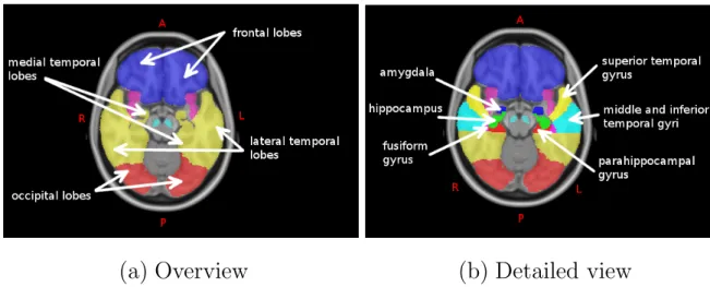
Pathological changes associated with the development of AD begin in the medial temporal lobes. Several important sub-structures within this region are illustrated in Figure 1.4.

(a) Overview

(b) Detailed view

Figure 1.4: Axial views of the brain, showing the sub-structures of the medial temporal lobe. A: anterior, P: posterior, L: left, R: right.

1.3

Neuropathology

Changes occur within the brain even during the healthy ageing process. For example, the cerebral hemispheres lose volume and the ventricles become enlarged. Both such changes may

1.3. Neuropathology 23

be attributed to neuronal loss (Graham and Lantos,1997). These changes become progressively exaggerated during the development of AD, with both cerebral atrophy and neuronal loss often more pronounced in the medial temporal lobes (Dawbarn and Allen, 2007). However, a more characteristic feature of the disease is the abundant presence in the brain of neuropathological structures including extracellular amyloid plaques and intracellular neurofibrillary tangles. For a diagnosis of definite AD to be returned, the presence and distribution of these structures must be directly examined in brain tissue samples.

Amyloid plaques are dense, insoluble deposits of protein and cellular material that form around neurons. Their main protein constituent is beta-amyloid (Aβ), which is produced when the larger amyloid precursor protein is successively cleaved byβ- andγ-secretase enzymes (Dawbarn and Allen, 2007). The dominant form of Aβ found in amyloid plaques is Aβ1−42. This is

produced when cleavage by γ-secretase occurs after residue 42 of the Aβ molecule, rather than the usual residue 40 (Selkoe, 2004). Once produced, Aβ proteins accumulate outside the cell, forming small, soluble oligomers. These then aggregate further and combine with other proteins and cellular material, eventually forming insoluble plaques (National Institute on Aging,2008). Neurofibrillary tangles are insoluble, twisted fibres found inside neurons, whose main protein constituent is the microtubule-associated protein tau. With the development of AD, the bal-ance between phosphorylation and dephosphorylation of tau is lost, and it becomes hyperphos-phorylated (Dawbarn and Allen, 2007). Tau and other microtubule-associated proteins then aggregate inside the cell, forming tangles. These disrupt the stability of the microtubules that are a vital part of the neuronal communication system, ultimately leading to cell death ( Na-tional Institute on Aging, 2008). The amyloid cascade hypothesis suggests that the formation of Aβ is directly responsible for triggering hyperphosphorylation of tau (Selkoe, 1991).

AD can be divided into two types which share the same pathological features: late-onset AD (LOAD) which tends to manifest after age 60, and the less common familial AD (FAD) which typically has an earlier onset (Dawbarn and Allen, 2007). The work presented in this thesis relates to cases of sporadic LOAD. Age is the most significant risk factor associated with the development of LOAD (Rocca et al., 1991), although genetic, environmental, and other

factors are also relevant. The ApoE gene is the only one so far shown to be associated with the development of LOAD (Dawbarn and Allen, 2007). There are three major alleles of the ApoE gene: 2, 3 and 4. The most common allele is 3, which is present in 70-80% of most populations (Zannis et al.,1981). The4 allele is associated with an increased risk of developing LOAD, while the 2 allele has a neuroprotective effect (Corder et al.,1993).

1.4

Neuroimaging

Neuroimaging techniques provide a way for clinicians to examine the structural and functional changes in the brain associated with the development of AD in vivo. Commonly used modal-ities include magnetic resonance imaging (MRI), X-ray computed tomography (CT), positron emission tomography (PET), single-photon emission computed tomography (SPECT), and dif-fusion tensor imaging (DTI). The work presented in this thesis will focus on PET and MRI, both of which are described in the following subsections.

1.4.1

Positron emission tomography

The basic procedure for a PET scan involves injecting the patient with a tracer, labelled with a positron-emitting radionuclide, and then scanning them. A positron emitted inside the body can travel only a short distance through tissue, losing kinetic energy by Coulomb scattering from atomic electrons as it does so, until it is almost at rest. When this low energy positron interacts with an atomic electron, the particles can annihilate to produce two gamma ray photons that are detectable outside the body. To conserve energy and momentum, the photons must be emitted in opposite directions and each with an energy of 511 keV. Since the elements of the PET detector form closed rings around the patient, the two photons are detected simultaneously in opposite detector elements. This process, known as coincidence detection, allows spatial localisation of the tracer in the body and the production of an image showing its distribution.

1.4. Neuroimaging 25

Radiotracers

Positron-emitting nuclei are unstable, and they stabilise by the decay of a proton into a neutron, positron and electron neutrino. The time taken for half the radioactive nuclei in a sample to decay is known as its half-life. Two nuclei commonly used in PET imaging are 11_{C and} 18_F,

which have half-lives of 20 and 110 minutes, respectively (Rudin, 2005). Tracer molecules for PET imaging are selected to target a particular physiological process, and then radiolabelled with a suitable positron-emitting nuclide. Isotopic labelling, such as the replacement of 12_{C by} 11_{C, is preferable because the resulting tracer has identical behaviour to the unlabelled molecule.}

However, labelling with 18F is attractive because its longer half-life means that synthesis of the tracer does not have to occur on-site. 18F is used as a pseudo-isotopic substitute for hydrogen in a variety of PET tracers because this exchange generally has only a small effect on the behaviour of the molecule in vivo.

Image acquisition

A PET scanner consists of a series of coaxial rings around the patient, each containing a number of detector elements. In the most commonly used detection systems, these elements are made up of an array of scintillating crystals which are optically coupled to location-sensitive photomultiplier tubes (Rudin,2005). When a gamma ray photon interacts with the scintillating crystal, electrons in the lattice are excited from the valence band up into the conduction band. These electrons return to the valence band at impurities in the crystal and, in doing so, dissipate energy in the form of light. This is converted into a weak electronic pulse which is then amplified into a measurable signal in the photomultiplier tubes.

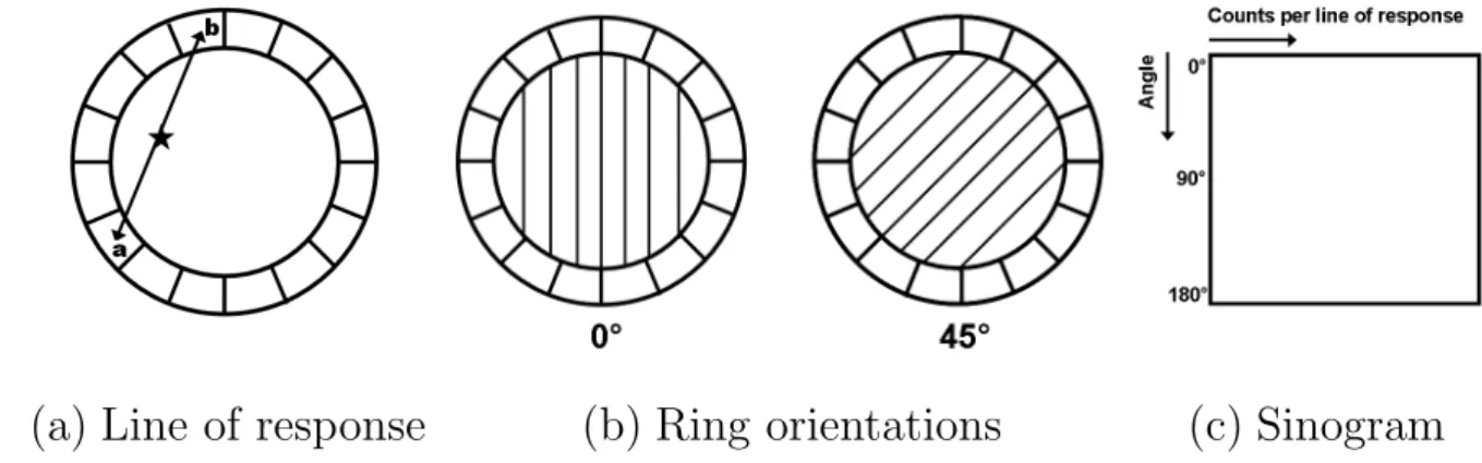
To describe how data are acquired, a single ring of the detector is considered in isolation. Each element in the ring is connected in a coincidence circuit with every other element, and an event is registered if photons are detected simultaneously in two elements. The detection of two photons must occur within a short coincidence window to be considered simultaneous. This is between 10 and 12 nanoseconds in modern clinical PET scanners (Rudin, 2005). Registration

of an event determines a path across the detector, known as the line of response, along which the two photons were emitted, as shown in Figure1.5 (a). Parallel lines of response are grouped together to form projections for every possible orientation of the ring, as illustrated in Figure

1.5 (b). The number of events recorded along each line of response in a single projection forms one row of a data matrix called a sinogram. The complete sinogram therefore contains information recorded from all projections in a single ring, as shown in Figure 1.5 (c).

(a) Line of response

(b) Ring orientations

(c) Sinogram

Photon attenuation in tissue

At energies around 511 keV, the dominant interaction of photons with tissue is by Compton scattering from outer-shell electrons. This results in both a loss of energy and deflection from the original path. Data must be corrected for errors occuring due to this attenuation, as well as other effects, before an image can be reconstructed. The probability that a photon undergoes no interactions as it travels through tissue along a line l is known as its survival probability. The survival probabilities of the pair of photons produced as shown in Figure

1.5 (a)are independent. The combined probability that neither photon interacts may therefore be expressed as PC = exp − Z b a µ(x)dx

1.4. Neuroimaging 27

for tissue with the linear attenuation coefficient µ(x) (Ollinger and Fessler, 1997). The atten-uation factor (1−PC) is thus independent of the position of the annihilation event along the

line l. It can be calculated for every line of response, and the resulting values used to correct the PET image for attenuation. The attenuation map may be obtained either from a transmis-sion scan acquired using an external radiation source prior to injection of the radiotracer, or from the CT image for combined PET/CT scanners. Not all attenuated photons are deflected out of the field of view, and an incorrect line of response may be registered if such scattered photons are detected. However, since energy loss is correlated with the angle of scatter, the registration of scattered photons may be suppressed by only considering those with sufficiently high energy (Rudin, 2005).

Image reconstruction

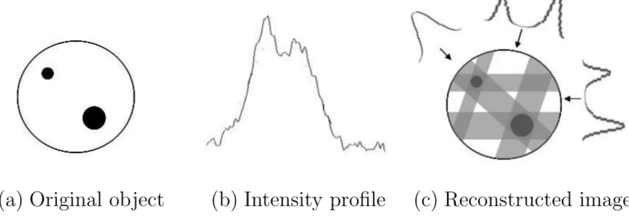
The aim of PET image reconstruction is to obtain a quantitative map of the spatial distribution of radiotracer in the body. A commonly used method is filtered back projection (FBP), which is described here by consideration of a single slice through an object, illustrated in Figure

1.6 (a). The projection at each angle is first extracted from the sinogram as an intensity profile, shown in Figure 1.6 (b). Since the angle at which each projection was acquired is known, the intensities can be back-projected to reconstruct the image, as shown in Figure 1.6 (c). The resulting star artefact can be suppressed by the application of a ramp filter (Jain,1989).

(a) Original object

(b) Intensity profile

(c) Reconstructed image

Iterative approaches may alternatively be used, such as the maximum likelihood expectation maximisation (MLEM) algorithm. This aims to find the image most likely to result in the observed projections, given some modelling of the data, noise and detection procedure. The algorithm begins with an estimate of the image, often that obtained using FBP, which it then modifies based on a comparison of the observed projections with those obtained from the image estimate (Qi and Leahy, 2006). In theory, this procedure is repeated until convergence, but in practice it can be very slow and a maximum number of iterations is often specified.

Image analysis

PET images may be acquired in static, dynamic, or gated modes. In static mode, images of sev-eral planes through the body provide visual information showing the radiotracer distribution. Although visual analysis can be a useful diagnostic tool, it lacks objectivity. Semi-quantitative objective measures may be obtained from static images. For example, the standardised uptake value (SUV) is the ratio of radioactivity in a region to a subject-specific scale factor which is determined from the injected dose and body weight of the patient (Rudin,2005). In some cases, there is a region in which the radiotracer accumulates to the same extent in both patients and healthy individuals. The SUV ratio (SUVR) between the region of interest and this reference region provides an alternative measure of regional radiotracer accumulation. In dynamic mode, a time-series of PET images is acquired, from which curves showing the regional tracer kinetics can be extracted. The temporal behaviour of the tracer can then be modelled, and pharma-cokinetic parameters derived. In gated mode, the image acquisition is synchronised with a physiological function, such as the cardiac cycle.

1.4.2

Magnetic resonance imaging

MRI exploits the phenomenon of nuclear magnetic resonance (NMR) to produce high quality structural images of the internal organs and other tissues. When undergoing a structural MRI scan, the patient is placed in a powerful static magnetic field, with which the spins of hydrogen

1.4. Neuroimaging 29

atoms in their body align. This alignment can be perturbed by the application of a radio frequency (RF) electromagnetic pulse, resulting in the resonance emission of a measurable RF signal. The strength of the static magnetic field determines the achievable image quality, and current clinical systems generally employ field strengths of 1.5 T or 3 T. Spatial localisation within the body is achieved by the application of magnetic field gradients, such that the static field varies in strength across the body. The frequency of the resonance signal detected there-fore becomes dependent on the location from which it was emitted. Different tissues can be distinguished by the characteristic properties of their emitted RF signals.

Nuclear magnetic resonance

Although nuclei behave according to the laws of quantum mechanics, the principles of NMR can be described with sufficient accuracy using a classical vector model in which nuclear spin is viewed as a physical gyroscopic rotation. In the presence of a static magnetic fieldB0, the spins

of hydrogen atoms in the body align either parallel or anti-parallel to the field, as illustrated in Figure 1.7. By convention, the coordinate system is defined such that B0 is oriented along

the z-axis. A net longitudinal magnetisation Mz results from the small excess of spins which

align in the lower energy parallel configuration. The spins precess about the static field at a frequency which is dependent on its strength. This is known as the Larmor frequencyωL =γB0,

where the gyromagnetic ratioγ is characteristic of the nuclei under consideration. The Larmor frequency for hydrogen atoms in the presence of a 1 T static field is 42.6 MHz (Becker,2000).

Figure 1.7: Hydrogen atoms in the presence of a static magnetic field B0, which induces a net

Since the spins do not precess in phase about the z-axis, there is no net magnetisation in the transverse plane. The application of a RF pulse oscillating at the Larmor frequency can establish phase coherence amongst the randomly precessing spins. The application of such a pulse perpendicular to the z-axis results in the rotation of the net magnetisation into the transverse plane. When the RF signal is then switched off, the spins precess in phase about the static magnetic field, thus inducing a measurable voltage in a receiver coil. The amplitude of this signal is maximal immediately following the RF pulse, but then decays with time as the precession loses phase coherence, and the system returns to equilibrium.

Fourier transforms

In the presence of a static magnetic field B0 oriented along the z-axis, the spins of hydrogen

atoms in the body precess in the xy-plane, as illustrated in Figure1.8 (a). This precession can be described by oscillating components in both the x- and y-directions, as shown in Figure

1.8 (b). A mathematical technique known as a Fourier transform can be used to convert these temporal signals into a frequency distribution. The temporal signals illustrated in Figure1.8 (b)

correspond to a single peak at the Larmor frequency, as illustrated in Figure 1.8 (c).

(a) Precession

(b) Temporal signals (c) Frequency distribution

The RF signal detected following resonance emission from nuclei within the body is a temporal signal consisting of many frequency components. A Fourier transform can convert this temporal

1.4. Neuroimaging 31

signal f(t) into a multi-spectral frequency distributionf(ω), according to the expression

f(ω) = Z ∞ −∞ f(t)e−iωtdt= Z ∞ −∞ f(t)[cos(ωt)−isin(ωt)]dt.

More detailed information about Fourier transforms and their properties may be found in

Jennison (1961). Spatial localisation

Spatial localisation is achieved by using magnetic field gradients to modify the static field so that it varies in strength across the body. Since the Larmor frequency is proportional to the applied magnetic field, the location of the source signal can then be inferred from the frequency of the resonance signal detected. Figure1.9depicts an example MRI pulse sequence illustrating the additional gradients required for spatial localisation in 3-D (Hornak, 2010).

Figure 1.9: An example MRI pulse sequence, showing the RF pulse, slice-selection gradientGS,

phase encode gradient Gφ, frequency encode gradient Gf, and the detected RF signal.

The application of a slice-selection gradientGS along the z-axis results in a Larmor frequency

which varies linearly with z. A RF pulse with a narrow band of frequencies therefore excites resonance within a single transverse section of the body. To achieve spatial localisation within this transverse section, additional gradients are applied along the x- and y-axes. A phase

encode gradient Gφ is first applied along one axis, such that the precession frequencies of the

nuclei within the transverse section become dependent on their position. When this gradient is switched off, the precession frequencies of the nuclei are once again identical; however, they precess out of phase. A frequency encode gradientGf is applied along the remaining axis during

the signal detection. The locations of nuclei within a transverse section of the body can then be unequivocally identified from the frequency distribution of the detected RF signal.

Tissue contrast

The decay of the RF signal as the nuclear spins return to equilibrium is associated with time constants describing its longitudinal and transverse components. Recovery of the longitudinal magnetisation as the spins realign with the static magnetic field is known as spin-lattice, or T1,

relaxation. Decay of the transverse magnetisation as the spins dephase is known as spin-spin, or T2, relaxation. Magnetic field inhomogeneities cause the signal to decay faster in the transverse

plane than can be explained byT2 relaxation alone. This effect is known asT2∗ relaxation. The

environment of the nuclei under consideration influences these time constants, and therefore the decay properties of the RF signal. MRI contrast is dependent on the differing T1 and T2

relaxation properties of various biological tissues.

1.5

Biomarkers for Alzheimer’s disease

Since the publication of the NINCDS-ADRDA Alzheimer’s Criteria in 1984, significant progress has been made in identifying the structural and molecular changes in the brain that are as-sociated with AD. Much of the recent research has been based on data from the Alzheimer’s Disease Neuroimaging Initiative (ADNI; http://adni.loni.ucla.edu), which aims to com-pare neuroimaging, biological, and clinical assessment of the cognitive and behavioural changes associated with normal ageing, MCI and AD. Participants undergo regular cognitive and func-tional assessments, and some also opted to undergo lumbar punctures for the collection of CSF biomarkers such as Aβ and tau. All ADNI participants had structural MRI scans, and

approx-1.5. Biomarkers for Alzheimer’s disease 33

imately 50% also underwent PET imaging with the tracer [18F]-fluorodeoxyglucose (FDG). Some participants additionally underwent PET imaging with the tracer [11_{C]-Pittsburgh}

com-pound B (PiB). FDG-PET images depict brain function in terms of the rate of cerebral glucose metabolism, and PiB-PET images show the distribution of amyloid deposition in the brain.

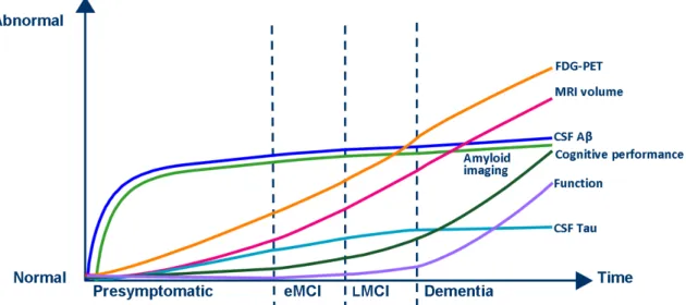
Figure1.10shows a hypothetical model of the temporal profiles of various biomarkers through-out the development of AD. Amyloid accumulation occurs earliest in the disease process, pre-ceding both cognitive and functional decline by years, and changing only gradually after symp-toms develop. Compared to measures of amyloid deposition, CSF tau levels, MRI volumes, and FDG-PET intensities are more dynamic biomarkers of AD progression. At present, a clinical diagnosis of AD is made based on assessments of cognition and behaviour, which start to decline fairly late in the disease process. Other biomarkers may therefore be better suited for the early detection and prediction of AD, and for monitoring progression. These are briefly reviewed in the following subsections.

Figure 1.10: Hypothetical temporal model of biomarker dynamics during AD progression. Biomarker measures vary from normal to maximally abnormal as a function of the disease stage. eMCI: early MCI, LMCI: late MCI. Adapted from (Aisen et al., 2010).

1.5.1

Cerebrospinal fluid

Recent consensus reports have identified CSF levels of Aβand tau as among the most promising potential AD biomarkers (Frank et al.,2003;The Ronald and Nancy Reagan Research Institute

of the Alzheimer’s Association and the National Institute on Aging Working Group, 1998). CSF levels of Aβ are approximately 100 times greater than those found in blood plasma, and this biomarker is best measured in the CSF (Scheuner et al., 1996). The same is true of tau, which is thought to be released from damaged neurons as they undergo neurofibrillary degeneration (Kahle et al., 2000). CSF is extracted by lumbar puncture, in which a needle is inserted between the lumbar vertebrae into the subarachnoid space of the spinal canal

Various studies have shown AD patients to have reduced CSF Aβ and elevated CSF tau com-pared with cognitively normal individuals (Ishiguro et al., 1999; Motter et al., 1995; Vander-meeren et al., 1993). When considered in combination, these two biomarkers can effectively distinguish AD patients from healthy individuals (Sunderland et al., 2003), as well as from patients with other types of dementia (Clark et al.,2003). AD patients with at least one ApoE 4 allele have lower CSF Aβ and higher CSF tau than those without (Tapiola et al., 2000). This finding aligns with the observation that more extensive AD pathology is generally found in AD carriers of the ApoE 4 allele than in non-carriers (Roses and Saunders, 1997).

MCI patients tend to have CSF Aβ and tau levels that lie between those expected of AD patients and healthy individuals. Preliminary data suggest that MCI patients with AD-like biomarker levels have a greater likelihood of converting to AD than those with biomarker levels more typical of cognitively normal individuals (Hansson et al., 2006). The first study of baseline CSF biomarker data from ADNI largely confirmed previous findings (Shaw et al.,

2009). CSF Aβ was found to be the most sensitive single CSF biomarker, and the overall best group discrimination was achieved by combining CSF Aβ and tau, along with the number of ApoE 4 alleles. The majority of MCI patients who converted to AD over the course of one year had baseline CSF Aβ and tau levels that were more typical of AD patients than of healthy controls.

1.5.2

Magnetic resonance imaging

The structural changes in the brain associated with AD can be non-invasively assessed using MRI. As shown in Figure 1.11, AD patients typically have evidence of cortical atrophy, and

1.5. Biomarkers for Alzheimer’s disease 35

enlarged ventricles in comparison with healthy individuals.

(a) Healthy individuals

(b) AD patients

Figure 1.11: Transverse sections from MR images of (a) healthy individuals, and (b) AD pa-tients. These images demonstrate that AD patients typically show evidence of cortical atrophy, and enlarged ventricles in comparison with healthy individuals.

Temporal lobe atrophy is closely associated with AD, and histological studies show that the hip-pocampus, amygdala and entorhinal cortex are particularly vulnerable to AD pathology (Braak and Braak, 1998). Correlation has been found between the rate of temporal lobe atrophy and both current cognitive performance and future decline, even among healthy individuals (Hua et al., 2008). Increased rates of hippocampal atrophy compared with cognitively normal in-dividuals have been measured using MRI in both AD and MCI patients (Schuff et al., 2009;

van de Pol et al., 2007). Longitudinal studies have additionally shown that the rate of hip-pocampal atrophy accelerates over time in both AD and MCI patients (Jack Jr. et al., 2008c;

Ridha et al.,2006). However, hippocampal atrophy alone is not sufficient to predict conversion from MCI to AD, and other structures may prove more sensitive (Dickerson et al., 2001). A recent analysis of the ADNI MRI data found that an increased rate of hippocampal volume

loss was associated with presence of the ApoE 4 allele in AD patients, and with reduced levels of CSF Aβ in MCI patients (Schuff et al., 2009). Another analysis showed that the rate of temporal lobe atrophy in AD is correlated with reduced CSF Aβ and elevated CSF tau, and that it is significantly faster in MCI subjects that later convert to AD than in non-converters (Leow et al., 2009).

1.5.3

Fluorodeoxyglucose positron emission tomography

FDG is a 18_{F labelled glucose analogue, whose distribution in the brain gives an indication of}

the cerebral metabolic rate of glucose (CMRgl). As shown in Figure1.12, AD patients typically have reduced glucose metabolism in temporo-parietal regions of the brain in comparison with healthy individuals.

(a) Healthy individuals

(b) AD patients

Figure 1.12: Transverse sections from FDG-PET images of (a) healthy individuals, and (b) AD patients. These images demonstrate that AD patients typically have reduced glucose metabolism in temporo-parietal regions of the brain in comparison with healthy individuals.

1.5. Biomarkers for Alzheimer’s disease 37

Numerous FDG-PET studies have shown that both MCI and AD are associated with significant reductions in the CMRgl in brain regions preferentially affected by the disease (de Leon et al.,

2001, 1983; Herholz et al., 2002; Langbaum et al., 2009; Mosconi et al., 2008, 2007; Mosconi,

2005; Nestor et al., 2003). AD patients display reductions of greater magnitude and spatial extent than MCI patients. Reductions in the CMRgl in AD patients can predict both their cognitive decline and histopathological diagnosis (Hoffman et al.,2000;Minoshima et al.,2001;

Silverman et al., 2001), while those in MCI patients can predict their conversion to AD ( An-chisi et al., 2005; Mosconi et al., 2004). Longitudinal studies have shown these changes to be progressive (Alexander et al., 2002; Mosconi et al., 2005). Based on comparisons of AD and MCI patients, it has been suggested that posterior regions are preferentially affected in the earlier stages of AD, with anterior regions such as the frontal cortex becoming involved only in the later stages of the disease (Alexander et al., 2002;Langbaum et al.,2009).

Cognitively normal individuals with one or two ApoE4 alleles already have reduced CMRgl in some of the regions affected by AD (Langbaum et al., 2009;Reiman et al., 2005). This finding suggests that FDG-PET can provide an early indicator for the disease. A single study of a small group of MCI patients (Drzezga et al., 2005) has demonstrated complete separation of those that rapidly converted to AD and those remaining stable, using a combination of reduced CMRgl in AD-typical regions and ApoE4 status.

1.5.4

Pittsburgh compound B positron emission tomography

PiB is a 11C labelled thioflavin-T derivative that binds to amyloid plaques in vivo. It can thus be used to assess one of the characteristic neuropathological features of AD. As shown in Figure1.13, AD patients typically have increased PiB retention in areas known to accumulate significant amyloid deposits in comparison with healthy individuals. A number of PiB-PET studies have reported cortical PiB retention in AD patients, and mostly non-specific retention in the white matter in healthy individuals (Forsberg et al., 2008; Jack Jr. et al., 2009; Klunk et al., 2004; Villemagne et al., 2008). Cortical PiB retention is also observed in MCI patients, but to a lesser extent than in AD. An inverse correlation has been found between cortical PiB

retention and levels of CSF Aβ (Fagan et al.,2006). Patients are often classified as PiB positive or negative, where a global cortical to cerebellar ratio is defined to separate the two groups. Independent studies have consistently found that approximately 30% of cognitively normal elderly individuals would be classified as PiB positive according to such criteria (Jack Jr. et al.,

2008b; Mintun et al., 2006). This suggests that PiB alone is not a sufficient marker for AD, although it may indicate individuals who will subsequently develop the disease. Longitudinal follow-up of cognitively normal PiB positive individuals will be required to verify this suggestion.

(a) Healthy individuals

(b) AD patients

Figure 1.13: Transverse sections from PiB-PET images of (a) healthy individuals, and (b) AD patients. These images demonstrate that AD patients typically show cortical PiB retention, while healthy individuals typically show non-specific retention in the white matter.

Significant amyloid plaque deposition occurs before the onset of clinical symptoms (Mintun et al.,2006), continuing at a slower rate as AD progresses. Progression may therefore be better assessed by considering measures of neurodegeneration. A study of ADNI MRI and PiB-PET found the rate of ventricular expansion greater in MCI patients that were PiB positive at baseline than in those that were PiB negative (Jack Jr. et al., 2009). This supports other studies suggesting that PiB negative MCI patients may not have early AD (Archer et al.,2006;

1.6. Research contributions and thesis outline 39

Forsberg et al., 2008). Additional follow-up data will again be required for verification.

1.6

Research contributions and thesis outline

The research presented in this thesis contributes to the growing body of literature surrounding the image-based classification of MCI and AD. In particular, a framework for multi-modality classification, based on the combination of similarity measures derived from random forest classifiers, is presented. In addition, early signs of neurodegeneration are identified in cognitively normal individuals at high risk of developing AD, based on multi-region analysis of MR images from two independent cohorts.

Relevant concepts from the fields of image analysis and machine learning are first described in Chapters 2 and 3, respectively. Chapter 2 describes image analysis techniques including regis-tration, anatomical segmentation, and statistical parametric mapping. Chapter3then provides an overview of machine learning concepts relevant to image-based classification, including clas-sification algorithms, and methods with which to assess their performance. A review of the current state-of-the-art for image-based classification of AD is additionally presented.

In terms of the classification of AD and MCI, there are many more studies based on structural MR imaging data than on FDG-PET imaging data. This is because anatomical imaging with either MRI or CT is routinely used in clinical practice for dementia patients. Investigations of the potential utility of multi-region FDG-PET features for image-based classification of AD and MCI are described in Chapters 4 and 5. In particular, attempts are made to distinguish between MCI patients who subsequently progress to AD and those who remain stable. Chapter

4demonstrates that regional information extracted from FDG-PET images acquired at a single timepoint can be used to achieve classification results in line with those obtained using data from MRI, or biomarkers obtained invasively from the CSF. Chapter 5 then demonstrates the additional benefit of incorporating longitudinal FDG-PET information for classification. By combining cross-sectional and longitudinal multi-region FDG-PET features, classification results in line with the current state-of-the-art are achieved. The findings described in these

chapters support the use of FDG-PET for the early diagnosis of AD and for monitoring its progression.

Changes in multiple neuroimaging and biological measures may provide complementary infor-mation for the diagnosis and prognosis of AD. Chapter6presents a multi-modality classification framework in which manifolds are constructed based on pairwise similarity measures derived from random forest classifiers. Similarities from multiple modalities are combined to generate an embedding that simultaneously encodes information about all the available features. Multi-modality classification is then performed using coordinates from this joint embedding. Random forests provide consistent pairwise similarity measures for multiple modalities, thus facilitating the combination of different types of feature data. Classification results based on the com-bination of regional MRI volumes, voxel-based FDG-PET signal intensities, CSF biomarker measures, and ApoE allele status are comparable with those obtained in other studies using multi-kernel learning. Since random forest classifiers extend naturally to multi-class problems, the framework described here could be used for other applications in the future, such as the differential diagnosis of AD.

Novel findings of early signs of neurodegeneration in cognitively normal individuals at high risk of developing AD are presented in Chapter 7. Multi-region analysis of MR images acquired at a single timepoint is used to show volumetric differences in cognitively normal individuals differing in amyloid-based risk status for the development of AD. Reduced volumes in temporo-parietal and orbito-frontal regions in high-risk individuals from two independent cohorts could be indicative of very early changes associated with AD. These findings suggest that volumetric MRI can reveal structural brain changes that precede the onset of clinical symptoms. It may therefore be useful in identifying early signs of neurodegeneration in healthy elderly individuals, potentially providing a useful early screening tool, or outcome measure for clinical trials.

Chapter 2

Background: PET and MR image

analysis

2.1

Introduction

This chapter describes state-of-the-art techniques relevant to the PET and MR image analysis presented in this work. Image registration is first described in Section 2.2. This allows the alignment of different images so that they share a common coordinate system. Anatomical segmentation techniques are then reviewed in Section 2.3. Much of the work presented in this thesis involves the use of multi-region imaging features obtained by using segmentation to label anatomically defined structures in the brain. The initial focus of this research was FDG-PET image analysis, and an overview of statistical parametric mapping is given in Section 2.4. This provides a voxel-based analysis method for studying group differences amongst PET images.

2.2

Image registration

The goal of image registration is to estimate a spatial correspondence between two images. Approaches can be broadly divided into those based on image intensity values, and those

which instead rely on image features such as lines or contours. The focus for this work is on intensity-based approaches. These typically comprise several related components: a transfor-mation model, optimisation method, similarity metric, regularisation method, and interpolation method. A transformation model defines the way in which one image (the source) should be deformed into the coordinate system of another (the target). Having selected a transformation model, the spatial correspondence between the two images is estimated by applying an optimi-sation method to find the transformation which maximises the image similarity. To ensure that the transformation is plausible, regularisation may be incorporated into the registration pro-cess. Finally, intensities may need to be interpolated to compensate for any mismatch between the deformed voxel grid of the source image and the target grid.

Several applications of image registration will be described in this thesis: alignment of images of a subject acquired at a single timepoint using different modalities (MRI and PET), alignment of images of a subject acquired serially using a single modality, and alignment to a standard template space of images of a group of subjects acquired using a single modality. Registration also forms part of an image segmentation procedure in which the labels from a set of manually segmented images are propagated to the target.

The components of the voxel-based registration method used throughout this research are de-scribed in detail in the following subsections. A more comprehensive review of image registration techniques may be found in Hajnal et al.(2001).

2.2.1

Transformation model

A transformation T defines a parametric representation mapping a voxel in the target image to a location in the source image, T : (x, y, z) → (x0, y0, z0). Transformations may be broadly divided into linear and nonlinear models. Linear models include both rigid transformations, which preserve distances between points, and affine transformations, which preserve colinearity of points. Linear transformations are global in nature, and cannot model local geometric differ-ences between images. Nonlinear (or nonrigid) transformations, however, can represent varying

2.2. Image registration 43

local deformations, thus allowing the source image to be locally warped into the coordinate system of the target.

The choice of transformation model is dependent on the application of interest. For example, a rigid transformation may be sufficient for the registration of serially acquired brain MR images of a healthy adult, since there should be very little change in the shape of the cranium. An affine transformation may be more appropriate for the intra-subject registration of brain MR and PET images acquired at a single timepoint, where some global scaling may be required. A nonrigid transformation may be applied following a global transformation to reduce any residual differences remaining between images. For example, local differences are likely to remain following global registration of serially acquired brain MR images of an AD patient.

Rigid transformations

A rigid transformation can be represented by the application of translations and rotations, as illustrated in Figure 2.1.

(a) Original image

(b) Translate

(c) Translate+Rotate

In 2-D, a translation in the xy-plane can be represented by a vector t, and rotations may be made about an axis perpendicular to the plane. An anti-clockwise rotation about thez-axis by an angle θ can be expressed as

Rz(θ) =    cosθ −sinθ sinθ cosθ   .

The effect of applying a rigid transformation comprising a rotation matrix R and translation vectortto a pointxcan be written asTrigid(x) = Rx+t. This may alternatively be represented

by the following single transformation matrix using homogenous coordinates:

Trigid(x) =    Rx+t 1   =    R t 0 1       x 1   ,

whereTrigidcan be decomposed into the following block form rotation and translation matrices:

Trigid =    R t 0 1   =    I t 0 1       R 0 0 1   .

In 3-D, a general rotation can be decomposed into rotations about each of the coordinate axes. In a right-handed frame, these rotations may be expressed as

Rx(θ1) =          1 0 0 0 0 cosθ1 −sinθ1 0 0 sinθ1 cosθ1 0 0 0 0 1          Ry(θ2) =          cosθ2 0 sinθ2 0 0 1 0 0 −sinθ2 0 cosθ2 0 0 0 0 1          Rz(θ3) =          cosθ3 −sinθ3 0 0 sinθ3 cosθ3 0 0 0 0 1 0 0 0 0 1          .

A general rotation comprising sequential rotations about thex-,y- andz-axes can be expressed as R = Rz(θ3)Ry(θ2)Rx(θ1). The single matrix representation for the rigid transformation

2.2. Image registration 45

Trigidis therefore the same as for the 2-D case. A general 3-D rigid transformation can therefore

be represented using six parameters, three describing translation, and three rotation.

Affine transformations

An affine transformation can be represented by the application of translations and rotations, as well as scales and shears, which are illustrated in Figure 2.2.

(a) Original image

(b) Scaling

(c) Shear

Figure 2.2: Illustration of possible affine transformations applied to (a) the original image, showing the effect of (b) scaling, and (c) shear.

In 3-D, scale factors sx, sy and sz can be applied independently along each of the coordinate

axes, such that a general scaling transformation may be expressed as

Tscale =          sx 0 0 0 0 sy 0 0 0 0 sz 0 0 0 0 1          .

In 2-D, shear along the x-direction describes the translation of a point x= (xx, xy) parallel to

the x-axis by an amountshxxy, whereshx is a scalar shear coefficient. Shear in the y-direction

can be similarly described by a scalar shear coefficient shy. The general shear matrix can then

Tshear =       1 shy 0 shx 1 0 0 0 1       .

In 3-D, shears can be characterised as either beam shears or slice shears, although these two representations are equivalent. A beam shear is defined as the translation of a point xparallel to one axis by an amount equal to a linear combination of the other two coordinate values. A slice shear involves translation of the point x along a pair of axes by an amount proportional to the coordinate value of the third. For example, shear along the x- and y-axes due to z is described by scalar shear coefficients shzx and shzy respectively. A general shear can therefore

be expressed as Tshear=          1 shxy shxz 0 shyx 1 shyz 0 shzx shzy 1 0 0 0 0 1          .

A general affine transformation may be expressed as Taffine = TshearTscaleTrigid. In 3-D,

translation, rotation and scale can each be represented using three parameters, and shear using six. It therefore appears that 15 parameters are required to specify an affine transformation. However, the parameters are not independent, and a general 3-D affine transformation may be expressed as Taffine =          a11 a12 a13 a14 a21 a22 a23 a24 a31 a32 a33 a34 0 0 0 1          .

2.2. Image registration 47

Nonrigid transformations

A nonrigid transformation represents local deformations which can vary across the image, as illustrated in Figure 2.3. There are various possible ways to characterise nonrigid transforma-tions because they require many more parameters than global transformatransforma-tions and therefore cannot be simply represented using a single matrix.

(a) Original image

(b) Deformed image

Figure 2.3: Illustration of a nonrigid transformation applied to (a) the original image, showing the effect of (b) a locally varying deformation.

A brief description of the relevant mathematical terminology is now presented. A function f on a domain Ω is described as continuous if an infinitesimal change in the input results in an infinitesimal change in the output. The class of all such continuous functions, whose nth derivatives are also continuous, is denoted Cn_{(Ω). If all derivatives of a continuous functionf}

are also continuous, the function is described as smooth, and it belongs to the class C∞(Ω). In practice, when modelling transformations, functions belonging to classes C2_{(Ω) and C}1_(Ω)

may be considered sufficently smooth. A function f which maps points from a set X to a set Y is described as a homeomorphism if it is a bijection, and both f and its inverse f−1 are continuous. A bijection describes an exact pairing of the setsX andY, such that each element inX is paired with exactly one element in Y, andvice-versa. A homeomorphic transformation preserves topology, and should therefore be used if the underlying topology between two images is assumed to be identical. Enforcing the additional restriction that both f and its inversef−1

must belong to the class Cn_{(Ω) defines f as a C}n_{-diffeomorphism. The term diffeomorphism}

is typically used to refer to the case of C∞-diffeomorphism. If the anatomical structures rep-resented within a pair of images are assumed to be smooth, the transformation between them

must be a diffeomorphism of the appropriate order. Diffeomorphic transformations are often used as a theoretical basis for the nonrigid registration of medical images.

A nonrigid transformation can be represented by a smooth displacement field, which requires the smooth assignment of vectors to every location in the image. In 3-D, this requires that a displacement vector is specified for every voxel, and the number of parameters is therefore three times the number of voxels. It is possible to reduce the number of parameters required by either using a model, or exploiting a property of the transformation. For example, a smooth transformation may be globally defined based on displacement vectors assigned to each of a set of control points defined within the image. For the free-form deformation (FFD) model used in this work (Rueckert et al., 1999), the control points are arranged on a regular nx×ny×nz

axis-aligned lattice with spacings δx, δy, δz along each coordinate axis. A FFD can then be

parametrised by a set of vectors {Φ}, each of which is associated with one of the control points. Displacement vector φi,j,k, for example, represents the control point located at position

x = (i, j, k). The nonrigid transformation is thus parametrised by the displacement vectors at the locations of the control points, but must also be defined at general locations within the image. This is achieved by convolving {Φ} with a suitable basis function, resulting in a smoothly varying displacement field across the entire image. In this work, the control points are convolved using 1-D cubic B-splines, which are expressed as

B0(u) = (1−u)3 6 B1(u) = (3u3_−6u2_{+ 4)} 6 B2(u) = (−3u3+ 3u2+ 3u+ 1) 6 B3(u) = u3 6 .

The local displacement at the general location x = (x, y, z) can then be written as the 3-D tensor product over the control point vectors, as

Tlocal(x, y, z) = 3 X l=0 3 X m=0 3 X n=0 Bl(u)Bm(v)Bn(w)φi+l,j+m,k+n,

where i=bx/δxc −1,j =by/δyc −1,k =bz/δzc −1, u=x/δx− bx/δxc,v =y/δy− by/δyc, w=z/δz− bz/δzc, and bxc= floor(x), which gives the largest integer not greater thanx.

2.2. Image registration 49

B-splines are computationally efficient because the displacement at a particular control point affects the transformation only in its local neighbourhood. Similarly, its displacement depends only on control points within the neighbourhood.

When performing nonrigid registration using FFDs, it is possible to employ a hierarchical, coarse-to-fine strategy (Schnabel et al., 2001) to reduce the likelihood of convergence to a local optimum. Using this approach, the FFD parameters are first optimised based on a relatively sparse control point lattice with a large spacing. This results in a transformation that captures large-scale local differences between the two images being registered. The control point lattice is then sub-divided to generate a lattice with half the spacing of the original (Forsey and Bartels,

1988). The FFD parameters are re-optimised based on this new, denser lattice of control points. This process of lattice sub-division and parameter optimisation may be repeated as required, with smaller-scale local differences between the images being captured at each iteration. It is important to ensure that the scale of the image features is appropriate for the selected control point spacing. The images should be blurred and resampled at each step so that information relating to structures smaller than a certain size is neglected. Images may be blurred by convolution with a Gaussian kernel of widthσ. For capturing large-scale differences, a relatively wide Gaussian kernel is appropriate. Successively smaller values of σ may then be selected as smaller-scale differences are captured by the FFD.

Combining global and local transformations

In the work presented in this thesis, nonrigid image registration is performed as a multi-stage process. Global transformation parameters are estimated, and used as the starting point for the nonrigid registration step. The global transformation itself is performed in two steps, with rigid transformation parameters estimated first, and used as the starting point for an affine registration. Rigid transformation parameters make up a su