Higher Order Recurrent Neural Network
for Language Modeling
Rohollah Soltani
a thesis submitted to
the faculty of graduate studies in partial fulfilment of the requirements
for the degree of Master of Science
graduate program in Electrical Engineering and Computer Science
York University Toronto, Ontorio
April, 2016
Abstract
In this thesis, we study novel neural network structures to better model long term dependency in sequential data. We propose to use more memory units to keep track of more preceding states in recurrent neural networks (RNNs), which are all recurrently fed to the hidden layers as feedback through different weighted paths. By extending the popular recurrent structure in RNNs, we provide the models with better short-term memory mechanism to learn long term dependency in sequences. Analogous to digital filters in signal processing, we call these structures as higher order RNNs (HORNNs). Similar to RNNs, HORNNs can also be learned using the back-propagation through time method. HORNNs are generally applicable to a variety of sequence modelling tasks. In this work, we have examined HORNNs for the language modeling task using two popular data sets, namely the Penn Treebank (PTB) and English text8 data sets. Experimental results have shown that the proposed HORNNs yield the state-of-the-art performance on both data sets, significantly outperforming the regular RNNs as well as the popular LSTMs.Acknowledgments
The past two years here at York University are the learning years of my life: not only my machines learn, but I learned a lot more. I appreciate it so much! This thesis would not have been possible without the support of many people. Firstly, I would like to express my sincere gratitude to my supervisor Prof Hui Jiang for the continuous support of my master study and related research, for his patience, motivation, and immense knowledge. His guidance helped me in all the time of research and writing of this thesis. I could not have imagined having a better advisor and mentor for my master study.I thank my fellow lab-mates and my friends in York University for the stimulating discussions and for all the fun we have had in the last two years.
Last but not the least, I would like to express my very profound gratitude to my family for supporting me spiritually throughout my years of study and my life in general. This accomplishment would not have been possible without them. Thank you.
Contents
Abstract ii
Acknowledgments iii
Table of Contents iv
List of tables vii
List of figures viii
Abbreviations ix
1 Introduction 1
1.1 Overview and motivation . . . 1
1.2 Contributions and Outline of the Thesis . . . 3
2 Neural Networks 6 2.1 Artificial neural networks . . . 6
2.2 Artificial neuron . . . 7
2.3 Feedforward Neural Networks . . . 10
2.4 Training Neural Networks . . . 13
3 Recurrent Neural Network 16 3.1 Recurrent Neural Network . . . 16
3.1.1 RNN Training . . . 19
3.2 Difficulties of training recurrent networks . . . 21
3.2.1 Hierarchical recurrent neural network . . . 22
3.2.2 Long short term memory . . . 23
3.2.3 Gated recurrent unit . . . 25
3.2.5 Other Variants . . . 28
4 Language modeling 31 4.1 Introduction . . . 31
4.2 Evaluating Language Models: perplexity . . . 32
4.3 N-gram . . . 33
4.4 Neural Language Model . . . 34
4.4.1 One hot representation . . . 35
4.4.2 Word Embedding . . . 36
4.4.3 Feed forward neural network based language model . . . . 36
4.4.4 Recurrent neural network based language model . . . 38
5 Higher Order Recurrent Neural Networks 40 5.1 Higher Order RNNs (HORNNs) . . . 41
5.1.1 Higher Order RNNs Training . . . 45
5.2 Pooling Functions for HORNNs . . . 46
5.2.1 Max-based Pooling . . . 48 5.2.2 FOFE-based Pooling . . . 49 5.2.3 Gated HORNNs . . . 49 6 Experiments 52 6.1 Experimental setup . . . 53 6.1.1 learning rate . . . 53 6.1.2 Weight decay . . . 54 6.1.3 Momentum . . . 54
6.1.4 Mini-batch gradient descent . . . 55
6.1.5 Max norm . . . 55
6.1.6 Weight Initialization . . . 56
6.1.7 Network architecture . . . 56
6.2 Language Modeling on PTB . . . 57
6.2.1 Effect of Orders in HORNNs . . . 57
6.2.2 HORNNs Complexity . . . 58
6.2.3 Effect of forgetting factor in FOFE HORNN . . . 59
6.2.4 Model Comparison on Penn TreeBank . . . 59
6.3 Language Modeling on English Text8 . . . 61
7 Conclusion 63 7.1 Conclusion . . . 63
List of Tables
6.1 Penn Treebank properties . . . 53 6.2 Perplexities on the PTB test set for various HORNNs . . . 58 6.3 Time complexity of HORNN models . . . 59 6.4 Perplexities on the PTB test set for various examined models. . . 61 6.5 Perplexities on the text8 test set for various models. . . 62
Listing of figures
2.1 The artificial neuron or perceptron . . . 8
2.2 Common Activation Functions . . . 10
2.3 Feedforward Neural Networks . . . 11
3.1 Recurrent neural network’s structure . . . 18
3.2 Recurrent neural network unfolded in time . . . 19
3.3 Back-propagation through time (BPTT) . . . 20
3.4 Long short term memory block . . . 25
3.5 Long short term memory . . . 26
3.6 Gated recurrent unit . . . 29
3.7 Clock-work RNN . . . 30
4.1 Forward neural network based language model . . . 37
4.2 Recurrent neural network based language model . . . 38
5.1 1st order and higher order RNN . . . 42
5.2 Unfolding a 3rd-order HORNN . . . 43
5.3 BPTT path for a 3rd-order HORNN . . . 44
5.4 Gradient flow in 3rd-order HORNN . . . 46
5.5 Pooling Functions for HORNNs . . . 47
5.6 Gated Hghier Order RNN . . . 50
Abbreviations
NN Neural Network
FNN Feed forward Neural Network
RNN Recurrent Neural Network
HORNN Higher Order Recurrent Neural Network
LSTM Long Sort Term Memory
GRU Gated Recurrent Unit
CWRNN Clockwork Recurrent Neural Network
BPTT Back propagation ThroughTime
FOFE Fixed-Size Ordinally Forgetting Encoding
If opportunity doesn’t knock, build a door.
Milton Berle
1
Introduction
1.1 Overview and motivation
In the recent resurgence of neural networks in deep learning, deep neural net-works have achieved huge successes in various real-world applications, such as speech recognition, computer vision and natural language processing. Deep neu-ral networks (DNNs) with a deep architecture of multiple nonlinear layers are
an extremely expressive model that can learn complex features and patterns in data. Each layer of DNNs learns some concepts and transfers them to the next layer and the next layer may continue to extract more complicated features, and finally the last layer generates the desirable output. From some early theoretical work [1, 2], it is well known that neural networks may be used as the so-called universal approximators to map from any fixed-size input to another fixed-size output. Recently, more and more empirical results have demonstrated that the deep structure in DNNs is not just powerful in theory but also can be reliably learned in practice from a large amount of training data.
Sequential modeling is a challenging problem in machine learning, which has been extensively studied in the past. Recently, many deep neural network based models have been very successful in this area, as shown in various tasks such as language modeling [3], sequence generation [4, 5], machine translation [6] and speech recognition [7]. Among various neural network models, recurrent neural networks (RNNs) are appealing for modeling sequential data because they can capture long term dependency in sequential data using a simple mechanism of re-current feedback [8]. RNNs can learn to model sequential data over an extended period of time, then carry out rather complicated transformations on the sequen-tial data. RNNs have been theoretically proved to be a turing complete machine [9]. RNNs in principle can learn to map from one variable-length sequence to an-other. When unfolded in time, RNNs are equivalent to very deep neural networks that share model parameters and receive the input at each time step. The recur-sion in the hidden layer of RNNs can act as an excellent memory mechanism for
the networks. In each time step, the learned recursion weights may decide what information to discard and what information to keep in order to relay onwards along time.
While RNNs are theoretically powerful, the learning of RNNs needs to use the so-called back-propagation through time (BPTT) method [10] due to the internal recurrent cycles. Unfortunately, in practice, it turns out to be rather difficult to train RNNs to capture long-term dependency due to the fact that the gradients in BPTT tend to either vanish or explode [11]. Many heuristic methods have been proposed to solve these problems. For example, a simple method, called gradient clipping, is used to avoid gradient explosion [3]. However, RNNs still suffer from the vanishing gradient problem since the gradients decay gradually as they are back-propagated through time. As a result, some new recurrent structures are proposed, such as long short-term memory (LSTM) [12] and gated recurrent unit (GRU) [13]. These models use some learnable gates to implement rather com-plicated feedback structures, which ensure that some feedback paths can allow the gradients to flow back in time effectively. These models have given promising results in many practical applications, such as sequence modeling [4], language modeling [14], hand-written character recognition [15], machine translation [13], speech recognition [7].
1.2 Contributions and Outline of the Thesis
In this work, we explore an alternative method to learn recurrent neural networks (RNNs) to model long term dependency in sequential data. We propose to use
more memory units to keep track of more preceding RNN states, which are all recurrently fed to the hidden layers as feedback through different weighted paths. Analogous to digital filters in signal processing, we call these new recurrent struc-tures as higher order recurrent neural networks (HORNNs). At each time step, the proposed HORNNs directly combine multiple preceding hidden states from various history time steps, weighted by different matrices, to generate the feed-back signal to each hidden layer. By aggregating more history information of the RNN states, HORNNs are provided with better short-term memory mechanism than the regular RNNs. Moreover, those direct connections to more previous RNN states allow the gradients to flow back more smoothly in the BPTT learning stage. All of these ensure that HORNNs can be more effectively learned to cap-ture long term dependency. Similar to RNNs and LSTMs, the proposed HORNNs are general enough for a variety of sequential modeling tasks. In this work, we have evaluated HORNNs for the language modeling task on two popular data sets, namely the Penn Treebank (PTB) and English text8 sets. Experimental results have shown that HORNNs yield the state-of-the-art performance on both data sets, significantly outperforming the regular RNNs as well as the popular LSTMs. The remainder of this thesis is organized as follows. In chapter 2, we will review the background in Neural Networks which is essential to understand the rest of the thesis. In chapter 3, the recurrent neural network will be introduced. In chapter 4, We will briefly review language modeling and neural network language modeling. In chapter 5, we first present the key idea of higher order RNNs (HORNNs) in detail, and then introduce several variant HORNN structures using different
pooling functions to generate the feedback signals. In chapter 6, we report and discuss the experimental results on two language modeling tasks. Finally, we conclude the thesis with our findings in chapter 7.
Anyone who stops learning is old, whether at 2 or 8. Anyone who keeps learning stays young. The greatest thing in life is to keep your mind young.
Moshe Arens
2
Neural Networks
2.1 Artificial neural networks
Artificial neural networks (ANNs) were originally developed as math-ematical models of the information processing abilities of biological brains [16]. The basic structure of an ANN is a network of small processing units, or nodes
(Artificial neuron), joined to each other by weighted connections. In terms of the original biological model, the nodes represent neurons, and the connection weights represent the strength of the synapses between the neurons. The network is acti-vated by providing an input to some or all of the nodes, and this activation then spreads throughout the network along the weighted connections. The electrical activity of biological neurons typically follows a series of sharp ‘spikes’, and the activation of an ANN node was originally intended to model the average ring rate of these spikes. Many varieties of ANNs have appeared over the years, with widely varying properties. One important distinction is between ANNs whose connec-tions form cycles, and those whose connecconnec-tions are acyclic. ANNs with cycles are referred to as feedback or recurrent, neural networks. ANNs without cycles are referred to as feed-forward neural networks (FNNs).
2.2 Artificial neuron
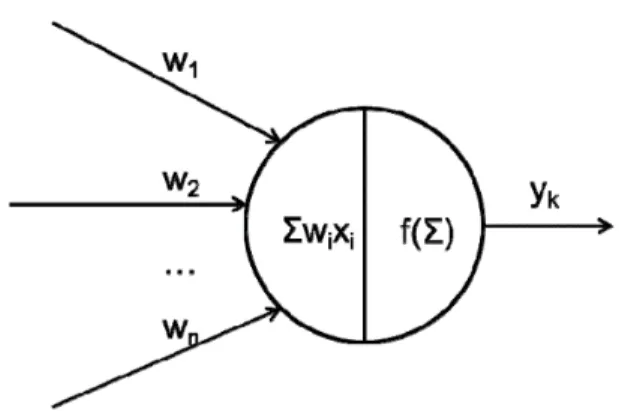
The artificial neuron or perceptron [17] is a simple computational unit that mimics the process of a biological neuron. However, it should be noted that the function-ality of a biological neuron is highly complex and still unclear. Perceptron is just a simple mathematical abstraction of how a biological neuron acts. Perceptron has scalar inputs and outputs. Each input has an associated weight which can be modified as the model training. The neuron multiplies each input by its weight, and then sums them, applies a activation function to the result, and passes it to its output.
func-Figure 2.1: The artificial neuron or perceptron
tion and the output. The output of the neuron is computed by the following function: y=f ( ∑ i Wixi+bi ) (2.1)
where xi is a scaler input, Wi is neuron weight and bi is bias. Let the inputs be
some n-dimensional vectorx. The output is computed by the following function:
y=f(Wtx+b) (2.2)
where f defines the activation function which can be any linear or non-linear transformation. Currently there is not any good theory to define which activation function is suitable in which conditions, and choosing the correct activation func-tion for a given task is most of the time an empirical quesfunc-tion. Few frequently used activation functions are:
input directly to the output.
f(a) =a (2.3)
Sigmoid (Sig): This activation function is an S-shaped function, transforming each value x into the range [0; 1].
f(a) = sigm(a) = 1
1+exp(a) (2.4)
Hyperbolic tangent (Tanh): This activation function is an S-shaped function, transforming the values x into the range [-1; +1]
f(a) = tanh(a) = exp(a)−exp(−a)
exp(a) +exp(−a) (2.5) Rectified linear units (ReLU): The rectifier activation function [18], is a very simple activation function that is easy to work with and has been shown many times to produce excellent results. The ReLU map all negative values into zero.
f(a) =Relu(a) =max(∅,a) (2.6) A single neuron described above can solve any linearly separable problem. more complex problem needs an structure of this neuron which will be described in the next sections.
(a)Linear activation function (b) Sigmoid activation function
(c) Tanh activation function (d) Relu activation function Figure 2.2: Common Activation Functions
2.3 Feedforward Neural Networks
Feedforward neural networks (FNNs) are a subset of ANNs whose nodes form an acyclic graph where information moves only in one direction, from input to output. A FNN consists of multiple layers with each layer being defined as a set of neurons.
Feed forward networks has two or more layers of neurons. Layer is a group of neurons receiving connections from the previous layer or the input. In FNNs neurons inside a layer are not connected to each other. A standard FNN as shown
in Figure 2.3 consist of three kinds of layers, an input layer, one or more hidden layers and an output layer.
Figure 2.3: Feedforward Neural Networks
-Input layer is the first layer of network and it does not receives any connections from other units, but instead it holds network’s input vector as output of its units and each input units is connected to every units in the hidden layer.
-Hidden layers can be considered as a projection of the input features onto some other feature space in such way it learns some concepts and transfers them to the next layer. Hidden layer is usually some nonlinear mapping of the input or the previous hidden layer. When we have more than one hidden layer, each hidden layer then is fully connected to the next hidden layer and the last hidden layer is fully connected to output layer. Given input X, the output of the hidden layer is defined as follows:
where W is the weight matrix, b is the bias vector and f is the hidden layer activation function.
-Output layer: Output layer is the last layer of the neural network and its output is the output of the network. The number of units in the output layer and its activation function depend on the task. Given the hidden layer activations (new features), the output layer compute the output f(x) as follow:
y=o(Wouth+b) (2.8)
where W is the weight matrix and b is the bias vector and o is the output activation function.
When we deal with a multiclass classification problem withk classes, the con-vention is to haveK output units, and normalize the output activations with the softmax function [19] which gives us a valid probability distribution over the k classes. The softmax activation function is defined as follows:
softmax(xi) =
exp(xi)
∑k
j=1exp(xj)
(2.9)
The result is a vector of non-negative real numbers that sum to one, making it a discrete probability distribution over k possible outcomes.
The universal approximation theorem [20] says that a three layer neural net-work can approximate any continuous function provided enough number of hidden units are used. However the number of required hidden units need to grow expo-nentially as the complexity of the problem increases.
To give more expressive power to neural networks with relatively smaller num-ber of hidden neurons, one obvious solution is to add more hidden layers which results in a highly non-linear transformation. One should note that adding more layers makes sense only if the hidden neurons have non-linear activation functions. In case of linear neurons, multiple hidden layers can be replaced by an equivalent single hidden layer with suitable weights and biases.
Since the output of an FNN depends only on the current input, and not on any past or future inputs, FNNs are more suitable for pattern classification than sequence labelling. We will discuss this point further in chapter 3.
All the weight in layers of neural network are the parameters of the model to be learnt. In the next section, we will discuss an efficient algorithm for learning these parameters.
2.4 Training Neural Networks
In the previous section, we described an artificial neuron and a network of neurons. In this section, we will see how to train them efficiently. The goal of neural network training is to optimize the weights in the network so that they cause the actual output to be closer to the the target output, thereby minimizing the network’s error and enable the neural network to correctly map arbitrary inputs to outputs. A neural network can be thought of as a function g that maps from input x to outputyvectors. The performance of the neural network is measured by a function called cost function. which calculates the deviation of the network output g(x) from the true output y. To train the neural network first the cost function of the
model should be computed and it has to be minimized during training. Some of the frequently used cost function are:
1: Squared error function
L=∥g(x)−y∥2 =∑
i
(g(xi)−yi)2 (2.10)
This is suitable when the output is a real value. 2: Negative log likelihood
L=−
N
∑
i
tilogg(xi) (2.11)
Where ti refers to the target probability which is set to 1.0 for the desired
output of the neural network, and0.0for all the other ones. This is suitable when the output is a probability distribution. In order to use this cost function, softmax activation functions need to be used in output layer.
Given a cost function, the training proceeds by learning all model parameters w(neurons weights in all layers) for the neural network so that the cost function over the training data is minimized. One of the popular algorithms to do this is the gradient descent method.
Using gradient decent the training process starts with a forward propagation of the sample input through the neural network in order to generate a network output. Then using the cost function the network’s error is computed and the contribution of each network parameters w to the error is computed by taking the gradient of the cost function with respect to the parameters. Finally the
parameters of the network is updated based on the gradient so that the training proceeds towards a local minimum of the cost function.
Δw= ∂L
∂w (2.12)
wnew=wold−λΔw (2.13)
where λ is the learning rate. The learning rate determines the magnitude of the step taken by gradient descent towards the local minimum. A larger learning rate corresponds with a faster training and a smaller learning rate with a more accurate training. Learning rate is one of the parameters that have to be chosen experimentally to achieve the best training performance.
The cost function for a feed forward neural network with multiple layers is a composition of several sub-functions and therefor deriving gradients with respect to each parameter is difficult. To efficiently calculate the gradient, a technique is introduced known as backpropagation algorithm for function compositions based on the chain rule for derivatives [21]. The idea of backpropagation is simple. When we train a neural network, we compute each layer output based on the input from the previous layer. Doing this computation from input to the output layer is known as forward propagation. Now we compute the gradient for the output layer and backpropagate the gradients until the input layer using the chain rule. This is computationally efficient.
The real problem is not whether machines think but whether men do.
B. F. Skinner
3
Recurrent Neural Network
3.1 Recurrent Neural Network
Recurrent neural networks (RNNs) are a subclass of artificial neural network that have at least one recurrent connection which make a loop in the network architec-ture. This recurrent connection is inspired by the cyclical connectivity of neurons in the brain uses iterative function loops to store information.
RNNs differ from FNNs due to their feedback loop, which allows information to be passed from one step of the network to the next. Therefore the output from each step is fed back to the network to affect the outcome of the next step (see Figure 3.1). FNNs accept only one input at a time and it is assumed that all inputs are independent of each other. However RNNs don’t have these constraints and can learn to map from one variable-length sequence to another. In principle FNNs makes a static model of the data given each new example, it can accurately classify or cluster them. In contrast, RNNs makes a dynamic model of the data that change over time and based on the context of the examples can accurately classify them.
Human’s memories are also aware of the context and use previous states to properly interpret new data. We don’t start thinking from scratch every second. As you read this thesis, you understand each word based on your understanding of previous words. You don’t throw everything away and start thinking from scratch again. Your thoughts have persistence.
This simple mechanism of recurrent feedback in RNNs allows the network to store an internal state and consequently process sequences of data and therefore capture long term dependency in sequential data [8]. The recurrent connections allow a ‘memory’ of previous inputs to persist in the network’s internal state, which can then be used to influence the network output. Theoretically, recurrent neural networks can store relevant information from previous time steps for an arbitrarily long period of time, making it possible to learn long-term dependencies. RNNs have been theoretically proved to be a turing complete machine [9]. When
(a)Recurrent neural network (b)one step unfolded Recurrent neural network
Figure 3.1: Recurrent neural network’s structure
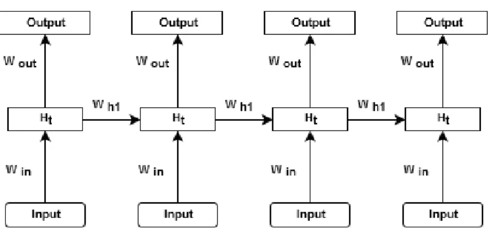
unfolded in time, RNNs are equivalent to very deep neural networks that share model parameters and receive the input at each time step (Figure 3.2). The recursion in the hidden layer of RNNs can act as an excellent memory mechanism for the networks. In each time step, the learned recursion weights may decide what information to discard and what information to keep in order to relay onwards along time.
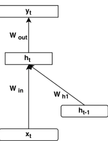
The forward pass of an RNN is the same as that of an FNN with a single hidden layer, except that activations arrive at the hidden layer from both the current input and the hidden layer activations from the previous time step. At each time stept, an RNN receives an inputxt and previous hidden state ht−1 , the
state of the RNN is updated recursively as follows (as shown in Figure 3.1):
Figure 3.2: Recurrent neural network unfolded in time
where f(·) is an nonlinear activation function, such as sigmoid or rectified linear units (ReLU), andWin is the weight matrix in the input layer andWh is the state
to state recurrent weight matrix. Due to the recursion, this hidden layer may act as a short-term memory of all previous input data.
Given the state of the RNN (the current activation signals in the hidden layer ht ), the RNN generates the output according to the following equation:
yt=g(Woutht) (3.2)
where g(·) denotes the softmax function and Wout is the weight matrix in the
output layer.
3.1.1 RNN Training
the standard backpropagation algorithm is not appropriate for networks that have cycles in them. Fortunately, a recurrent neural network which is used for N time
steps can be seen as a deep feed-forward network with N hidden layers by unfolding the network in time as shown in Figure 3.3. However, unlike a normal hidden layer, each hidden layer also takes an input (the input into the neural network at that time step). Thus, the network actually has N+1 different inputs: an initial hidden state and N inputs, one per time step.
Figure 3.3: back-propagation through time (BPTT)
This deep feed-forward network now can be trained by the normal gradient descent as discussed before. Errors are propagated recursively from each hidden layer to its previous time step and the recurrent weight matrix is updated. This
method of learning RNN networks is referred to as back-propagation through time (BPTT) [10].
The unfolding can be applied for as many time steps as many training examples were already seen. However usually a few step is enough because the gradient vanish as it back-propagate through time.
3.2 Difficulties of training recurrent networks
While RNNs are theoretically powerful unfortunately, in practice, it turns out to be rather difficult to train RNNs to capture long-term dependency. It is due to the fact that the gradients in the back-propagation process tend to either, decays or blows up exponentially and do not reach earlier input signals [11]. Therefore the influence of the given input on hidden layer and output layer will vanish or explode as it cycles around the recurrent connection of the RNN. Many heuristic methods have been proposed to solve these problems. It turned out that gradient explosion can be avoided by a simple yet efficient method, calledgradient clipping
[3]. The norm of the gradient of the cost respect to the parameters is computed. If the gradient’s norm is greater than a predefined threshold t, the norm of the gradient will be renormalized to be equal to t. Otherwise, it is leaved as it is. However, RNNs still suffer from the vanishing gradient problem since the gradi-ents decay gradually as they are back-propagated through time. This makes the internal states of the RNNs focused only on short term patterns, practically ignor-ing longer term dependencies. There are two reasons for this phenomena. First, the derivation of standard activation functions like the sigmoid and tanh function
is close to zero almost everywhere. This issue has been partially solved in deep neural networks by using the rectified linear units (ReLU) [22]. Second, as the gradient is back-propagated through time, its magnitude is multiplied over and over by the recurrent weight matrix. If the eigenvalues of this matrix are smaller than one, the gradient will converge to zero exponentially. In practice, gradients are usually close to zero after 5 – 10 steps of backpropagation. This makes it hard for simple recurrent neural networks to learn tasks containing delays of more than about 10 time-steps between relevant input and target [23].
As a result, some new recurrent structures are proposed, such as long short-term memory (LSTM) [12] and gated recurrent unit (GRU) [13]. These models use some learnable gates to implement rather complicated feedback structures, which ensure that some feedback paths can allow the gradients to flow back in time effectively. These models have yielded promising results in many practical applications, such as sequence modeling [4], language modeling [14], hand-written character recognition [15], machine translation [13], speech recognition [7].
3.2.1 Hierarchical recurrent neural network
Hierarchical recurrent neural network proposed in [24] is one of the earliest papers that attempt to improve RNNs to capture long term dependency in a better way. It proposes to add linear time delayed connections to RNNs to improve the gradient descent learning algorithm to find a better solution, eventually solving the gradient vanishing problem. However, in this early work, the idea of multi-resolution recurrent architectures has only been preliminarily examined for some
simple small-scale tasks. This work is somehow relevant to our work in this thesis but the higher order RNNs proposed here differs in several aspects. Firstly, we propose to use weighted connections in the structure, instead of simple multi-resolution short-cut paths. This makes our models fall into the category of higher order models. Secondly, we have proposed to use various pooling functions in generating the feedback signals, which is critical in normalizing the dynamic ranges of gradients flowing from various paths. Our experiments have shown that the success of our models is largely attributed to this technique.
3.2.2 Long short term memory
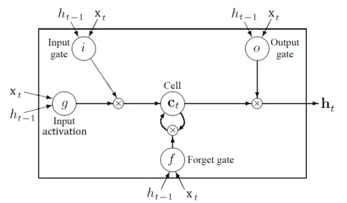
The most successful approach to deal with vanishing gradients so far is to use long short term memory (LSTM) model [12]. LSTM relies on a fairly sophisti-cated structure made of gates to control flow of information to the hidden neurons. As shown in Figure 3.4 There are three gates, i, f and o, controlling for input, forget and output. They have the exact same equations, just with different pa-rameter matrices. The gate values are in the range [0; 1] computed based on linear combinations of the current inputxt and the hidden layer’s previous states ht−1 ,
passed through a sigmoid activation function. The input gate controls how much information about the new input should be written to the memory cell. While the forget gate decides how much information from the memory cell should be forgotten, and the output gate decides how much of the memory cell should be revealed to the network. The output of the LSTM network will be computed as follow:
Gates: i=sigma(x×Wxi+ht−1×Whi) o=sigma(x×Wxo+ht−1×Who) f=sigma(x×Wxo+ht−1×Who) Input activation: g=tanh(x×Wxg+ht−1×Whg) State update: ct=ct−1⊙f+g⊙i ht=tanh(ct)⊙o
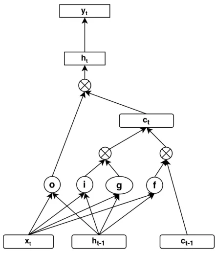
Implementation view of the LSTM can be pictured like Figure 3.5. Here i,f and o are the gates and g is a candidate hidden state. All of them are computed based on the current input and the previous hidden state. ct is internal memory
of the network which is combination of the candidate hidden stategmultiplied by input gateiand previous internal memory stateCt−1 multiplied by the forget gate
f. therefor it is the combination of the amount of the memory we want to stay in the network and the new candidate generated.
Figure 3.4: Long short term memory block
retrieve information over long periods of time, thus avoiding the vanishing gradient problem. For instance, as long as the input gate remains closed (has an activation close to zero), the status of the cell will not be overwritten by the new inputs arriving in the network, and can be made available to the network much later in the sequence, by opening the output gate. The drawback of the LSTM is that it is complicated and slow to learn. The complexity of this model makes the learning very time consuming, and hard to scale for larger tasks.
3.2.3 Gated recurrent unit
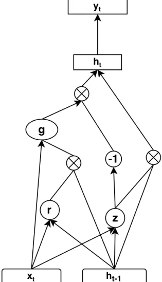
The LSTM architecture is very effective, but also quite complicated. The com-plexity of the system makes it hard to analyze, and also computationally expensive to work with. The gated recurrent unit (GRU) [13] was recently introduced as
Figure 3.5: Long short term memory structure
an alternative to the LSTM. The GRU model is found to outperform the LSTM on some language modeling and machine translation tasks. The GRU similar to the LSTM, is based on a gating mechanism to learn long-term dependencies, but with just two gates (reset gate and update gate) and without a separate internal memory. The output of the GRU is computed as follow:
r=sigma(x×Wxr+ht−1×Whr)
z=sigma(x×Wxz+ht−1 ×Whz)
g=tanh(x×Wxg+ (r⊙ht−1)×Whg)
ht=z⊙ht−1 + (1−z)⊙g
As shown in figure 3.6 the reset gate (r) is used to control access to the previous state and determined how to combine it with the input. The update gate (z) based on an interpolation determine how much of the previous memory to keep in the network.
3.2.4 Clock-work RNNs
Recently, clock-work RNNs [25] are proposed to address this problem as well, which splits each hidden layer into several modules running at different clocks as shown in Figure 3.7 . Each module receives signals from input and computes its output at a predefined clock rate. Module is fully connected within but connec-tions across modules are restricted. Nodes in one module are connected to other module only if it is relatively faster. This mechanism allows slower modules to focus on long-term, while faster modules focus on short-term information. Gated feedback recurrent neural networks [26] attempt to implement a generalized ver-sion of clock-work RNN using the gated feedback connection between layers of stacked RNNs, allowing the model to adaptively adjust the connection between
consecutive hidden layers.
3.2.5 Other Variants
Some researchers explore simpler architectures to address this issue. One of these approaches is to add a context layer to RNNs [27]. This layer is responsible for capturing longer term dependencies in input data by making its weight matrix close to identity. They observed that the recurrent connection of the RNN changes largely at each time step, prohibiting it from remembering information over long time periods. Therefore they proposed to add a slow-changing context layer to the network, in this way, both short and longer dependency information can be captured.
More recently, some short-cut skipping connections have been found useful in learning very deep feed-forward neural networks as well, such as [28,29,30]. These skipping connections between various layers of neural networks can improve the flow of information in both forward and backward passes. Among them, highway networks [31] introduce rather sophisticated skipping connections between layers, controlled by some gated functions.
without language, one cannot talk to people and understand them, one cannot share their hopes and aspirations, grasp their history, appreciate their poetry, or savour their songs.
Nelson Mandela
4
Language modeling
4.1 Introduction
Language modelingis a fundamental task in many natural language processing (NLP) applications such as machine translation [32], automatic speech recognition [33] , response generation [34] and information retrieval [35].
A language model assign a probability distribution over a various linguistic units, e.g., words that captures statistical regularities of natural language [36]. Thus syntactically and semantically reasonable sentences receive high probabili-ties.
The goal of statistical language modeling is to predict the next word in textual data given context; thus we are dealing with sequential data prediction problem when constructing language models.
The probability of a sequence of symbols (usually words) is computed using a chain rule as P(w) = N ∑ i=1 P(wi |w1· · ·w(i−1)) (4.1)
4.2 Evaluating Language Models: perplexity
To evaluate the performance of language models, an appropriate evaluation metric is needed. The most commonly used measure for language models is perplexity (PPL). The perplexity of a language model is calculated as the geometric average of the inverse probability of the words on the test data: Calculation of the per-plexity can be interpreted as evaluating how difficult it is for the language model to predict the next word in a word sequence. The perplexity is a positive number. The lower the perplexity, the better the model is at modeling unseen data.The perplexity of a language model P is defined as
PPL= k v u u t∏k i=1 1 P(wi |w(1···i−1) ) =2−k1 ∑k i=1log2P(wi|w(1···i−1)) (4.2)
4.3 N-gram
The most frequently used language models are based on the count-based n-gram, which are basically word co-occurrence frequencies. It intends to assign the prob-ability distribution of a given word observed after a fixed number of previous words. The maximum likelihood estimate of probability of word A in context H is computed as
P(A|H) = C(HA)
C(H) (4.3)
Whereh=w1,w2,· · · ,wkis called history or context andC(HA)denote the number
of times that theHA sequence of words has occurred in the data. The contextH can consist of several words, for the usual trigram models |H| = 2. For H = 0, the model is called unigram, and it does not take into account history.
However, there is a severe problem in n-gram modeling caused by its frequency counts. When confronted with words that have not been seen in the training corpus in a particular context H, the probability becomes zero. This happens because of the sparseness of data since the training corpus is always limited. In this situation smoothing techniques need to be applied to address this issue. This works by redistributing probabilities between seen and unseen (zero-frequency) n-gram and assigning a small probability to all unseen n-n-grams. Detailed overview of common smoothing techniques and empirical evaluation can be found in [37]
The most important factors that influence quality of the resulting n-gram model is the choice of the order and of the smoothing technique. The most sig-nificant advantages of models based on n-gram statistics are speed (probabilities
of n-grams are stored in precomputed tables), reliability coming from simplicity, and generality (models can be applied to any domain or language effortlessly, as long as there exists some training data). N-gram models are today still consid-ered as state of the art not because there are no better techniques, but because those better techniques are computationally much more complex, and provide just marginal improvements, not critical for the success of given applications.
The weak part of n-grams is slow adaptation rate when only limited amount of in-domain data is available. The most important weakness is that the number of possible n-grams increases exponentially with the length of the context, preventing these models to effectively capture longer context patterns. This is especially painful if large amounts of training data are available, as much of the patterns from the training data cannot be effectively represented by n-grams and cannot be thus discovered during training. The idea of using neural network based LMs is based on this observation, and tries to overcome the exponential increase of parameters by sharing parameters among similar events, no longer requiring exact match of the history H.
4.4 Neural Language Model
Neural networks have been widely considered as the most promising technique for language modeling after Bengio et. al. publish their feed forward neural network language model(NNLM) [38]. Since then neural network based models are able to get much better result than n-gram models even with small datasets. The main advantage of NNLMs over n-grams is that history is no longer seen as exact
sequence of words, but rather as a projection of them into some lower dimensional continuous space. This decreases significantly the number of parameters in the model that have to be trained, resulting in automatic clustering of similar histories and mapping discrete words into a continuous space where similar context are near each other. The main drawback of these models is their computational complexity, which usually make it hard to train these models on large training set, using the full vocabulary.
4.4.1 One hot representation
The train and test data for modeling a language are sequence of words. To rep-resent this word to the network a unique number is assigned to each word and the representation of the word is a vector of mostly zeros with just a one in the position of the word’s number. This technique assures the network get inputs without any prior knowledge of the words and each word will be in equal distance away from others words. Mathematically each word I in the vocabulary V is rep-resented as a binary vectorXi whose i-th element is one and all other element are
set to zero.
Xi = [0000· · ·0 1|{z} i−th
000· · ·00]
This representation is called one-hot representation and has been wildly used in neural network language modeling.
4.4.2 Word Embedding
Next step in most of the NNLMs is building the embedding layer which project the inputs to some low dimensional continuous space. Let us see what it means to multiply the weight matrix with an one-hot vector. Since only one of the elements of the one-hot vector is non-zero, all the rows of the matrix will be ignored except for the row corresponding to the index of the non-zero element of the one-hot vector. This row is multiplied by 1, which simply gives us the same row as the result of this whole matrix–vector multiplication. In short, the multiplication of the weight matrix with an one-hot vector is equivalent to slicing out a single row from the matrix.
This view has two consequences. First, in practice, it will be much more effi-cient computationally to implement this multiplication as a simple table look-up. Second, from this perspective, we can see each row of the matrix as a continuous-space representation of a corresponding word. Each row will be a vector repre-sentation of the i-th word in the vocabulary V. This reprerepre-sentation is often called a word embedding and should reflect the underlying meaning of the word.
4.4.3 Feed forward neural network based language model
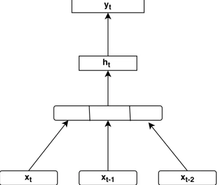
The original model of feed-forward neural network based language model pro-posed by Bengio [38] , which are depicted in Figure 4.1 as follows: the input of the feed forward NNLM is formed by using a fixed length history of previous n-1 words, where each of the previous n-1 words is encoded using one-hot representa-tion, using embedding layer each word in the vocabulary is mapped by a shared
parameter matrix to a real-valued vector. Following the projection layer is the hidden layer and After that is the softmax output layer with the size equal to the size of full vocabulary. The output is the conditional probabilities of current word given its previous n-1 words.
Figure 4.1: forward neural network based language model
Feed forward Neural Networks usually represent time explicitly with a fixed-length window of the recent history. While this type of models work well in practice, fixing the window size makes long-term dependency harder to learn and can only be done at the cost of a linear increase in the number of parameters.
4.4.4 Recurrent neural network based language model
Language modeling achieve a bigger improvement when mikolov et. al. [3] pro-posed to use recurrent neural networks in language modeling. The main difference between the feed-forward and the recurrent architecture is in representation of the history. While for feed-forward NNLM, the history is just previous several words, for the recurrent model, the representation of history is learned from the data during training. The hidden layer of RNN represents all previous history and not just n-1 previous words, thus the model can theoretically represent long context patterns. In simple recurrent networks, the state of the hidden layer at a given time is conditioned on its previous state. This recursion allows the model to store complex patterns for longer time periods.
(a)Recurrent neural network (b) Unfolded recurrent neural network
Figure 4.2: Recurrent neural network based language model
Figure 4.2 depicts the RNNLM architecture model. The input layer consists of a vector xt that represents the one-hot representation of the current word and
of vectorh(t−1)that represents a copy of previous activated hidden layerh after the network is trained, the output layer y(t) represents P(x(t+1)|xt,h(t−1)
) .
Start by doing what’s necessary; then do what’s possible; and suddenly you are doing the impos-sible.
Francis of Assisi
5
Higher Order Recurrent Neural Networks
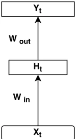
A recurrent neural network (RNN) is a type of neural network suitable for modeling a sequence of arbitrary length. At each time stept, an RNN receives an input xt, the state of the RNN is updated recursively as follows (as shown in
the left part of Figure 5.1):
ht=f(Winxt+Whht−1) (5.1)
where f(·) is an nonlinear activation function, such as sigmoid or rectified linear (ReLU), and Win is the weight matrix in the input layer and Wh is the state to
state recurrent weight matrix. Due to the recursion, this hidden layer may act as a short-term memory of all previous input data.
Given the state of the RNN, i.e., the current activation signals in the hidden layerht, the RNN generates the output according to the following equation:
yt=g(Woutht) (5.2)
whereg(·) denotes the softmax function andWout is the weight matrix in the
out-put layer. In principle, this model can be trained using the back-propagation through time (BPTT) algorithm [10]. This model has been used widely in se-quence modeling tasks like language modeling [3].
5.1 Higher Order RNNs (HORNNs)
RNNs are very deep in time and the hidden layer at each time step represents the entire input history, which acts as a short-term memory mechanism. However, due to the gradient vanishing problem in back-propagation, it turns out to be very difficult to learn RNNs to model long-term dependency in sequential data.
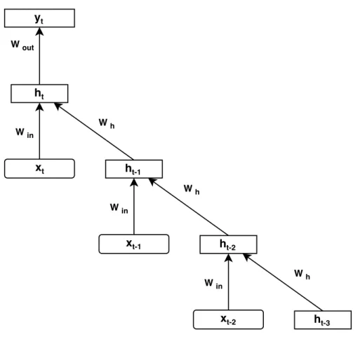
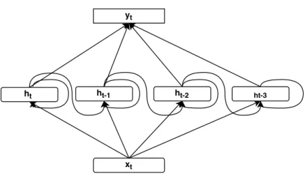
long-Figure 5.1: Comparison of model structures between an RNN (1st order) and a higher order RNN (3rd order). The symbolz−1 denotes a time-delay unit (equivalent to a memory unit).
term dependency in sequential data. As shown in the right part of Figure 5.1, instead of using only the previous RNN state as the feedback signal, we propose to employ multiple memory units to generate the feedback signal at each time step by directly combining multiple preceding RNN states in the past, where these time-delayed RNN states go through separate feedback paths with different weight matrices. Analogous to the filter structures used in signal processing, we call this new recurrent structure as higher order RNNs, HORNNs in short. The order of HORNNs depends on the number of memory units used for feedback. For example, the model used in the right of Figure 5.1 is a 3rd-order HORNN. On the other hand, regular RNNs may be viewed as 1st-order HORNNs.
In HORNNs, the feedback signal is generated by combining multiple preceding RNN states. Therefore, the state of anN-th order HORNN is recursively updated
as follows: ht =f ( Winxt+ N ∑ n=1 Whnht−n ) (5.3)
where {Whn | n =1,· · ·N} denotes the weight matrices used for various feed-back paths.
Figure 5.2: Unfolding a 3rd-order HORNN
Similar to RNNs, HORNNs can also be unfolded in time to get rid of the recur-rent cycles. As shown in Figure 5.2, we unfold a 3rd-order HORNN in time, which clearly shows that each HORNN state is explicitly decided by the current inputxt
and all previous 3 states in the past. This structure looks similar to the skipping short-cut paths in deep neural networks but each path in HORNNs maintains a learnable weight matrix. The new structure in HORNNs can significantly improve the model capacity to capture long-term dependency in sequential data. At each
Figure 5.3: Illustration of all back-propagation paths in BPTT for a 3rd-order HORNN.
time step, by explicitly aggregating multiple preceding hidden activities, HORNNs may derive a good representation of the history information in sequences, leading to a significantly enhanced short-term memory mechanism [39].
During the back-propagation learning procedure, these skipping paths directly connected to more previous hidden states of HORNNs may allow the gradients to flow more easily back in time, which eventually leads to a more effective learning of models to capture long term dependency in sequences. Therefore, this structure may help to largely alleviate the notorious problem of vanishing gradients in the RNN learning.
5.1.1 Higher Order RNNs Training
Obviously, HORNNs can be learned using the same BPTT algorithm as regular RNNs, except that the error signals at each time step need to be back-propagated to multiple feedback paths in the network. As shown in Figure 5.3, for a 3rd-order HORNN, at each time step t, the error signal from the hidden layer ht will have
to be back-propagated into four different paths: i) the first one back to the input layer, xt; ii) three more feedback paths leading to three different histories in time
scales, namely ht−1, ht−2 and ht−3. A higher order recurrent neural network which
is used for N time steps can be seen as a deep feed-forward network with N hidden layers by unfolding the network in time as shown in figure 5.4.
Interestingly enough, if we use a fully-unfolded implementation for HORNNs as in Figure 5.2, the overall computation complexity is comparable with regular RNNs. Given a whole sequence, we may first simultaneously compute all hidden activities (fromxt toht for allt). Secondly, we recursively update ht for alltusing
Eq.(5.3). Finally, we use GPUs to compute all outputs together from the updated hidden states (from ht to yt for all t) based on eq.(5.2). The backward pass in
learning can also be implemented in the same three-step procedure. Except the recursive updates in the second step (this issue remains the same in regular RNNs), all remaining computation steps can be formulated as large matrix multiplications. As a result, the computation of HORNNs can be implemented fairly efficiently using GPUs.
Figure 5.4: back-propagation flow in BPTT for a 3rd-order HORNN.
5.2 Pooling Functions for HORNNs
As discussed above, the shortcut paths in HORNNs may help the models to cap-ture long-term dependency in sequential data. On the other hand, they may also complicate the learning in a different way. Due to different numbers of hidden layers along various paths, the signals flowing from different paths may vary dra-matically in the dynamic range. For example, in the forward pass in Figure 5.2,
three different feedback signals from different time scales, e.g. ht−1, ht−2 and ht−3,
flow into the hidden layer to compute the new hidden stateht. The dynamic range
of these signals may vary dramatically from case to case. The situation may get even worse in the backward pass during the BPTT learning. For example, in a 3rd-order HORNN in Figure 5.2, the node ht−3 may directly receive an error
sig-nal from the node ht. In some cases, it may get so strong as to overshadow other
error signals coming from closer neighbours ofht−1 and ht−2. This may impede the
learning of HORNNs, yielding slow convergence or even poor performance.
Figure 5.5: A pooling function is used to calibrate various feedback paths in HORNNs.
Here, we have proposed to use some pooling functions to calibrate the sig-nals from different feedback paths before they are used to recursively generate a new hidden state, as shown in Figure 5.5. In the following, we will investigate three different choices for the pooling function in Figure 5.5, includingmax-based pooling, FOFE-based pooling and gated pooling.
5.2.1 Max-based Pooling
Max-based pooling is a simple strategy that chooses the most responsive unit (exhibiting the largest activation value) among various paths to transfer to the hidden layer to generate the new hidden state. Many biological experiments have shown that biological neuron networks tend to use a similar strategy in learning and firing.
In this case, instead of using eq.(5.3), we use the following formula to update the hidden state of HORNNs:
ht=f
(
Winxt+maxNn=1 (Whnht−n)
)
(5.4)
where maximization is performed element-wisely to choose the maximum value in each dimension to feed to the hidden layer to generate the new hidden state. The aim here is to capture the most relevant feature and map it to a fixed predefined size.
The max pooling function is simple and biologically inspired. However, the max pooling strategy also has some serious disadvantages. For example, it has no forgetting mechanism and the signals may get stronger and stronger. Furthermore, it loses the order information of the preceding histories since it only choose the maximum values but it does not know where the maximum comes from.
5.2.2 FOFE-based Pooling
The so-called fixed-size ordinally-forgetting encoding (FOFE) method was pro-posed in [40] to encode any variable-length sequence of data into a fixed-size representation. In FOFE, a single forgetting factor α (0 < α < 1) is used to encode the position information in sequences based on the idea of exponential forgetting to derive invertible fixed-size representations. In this work, we borrow this simple idea of exponential forgetting to calibrate all preceding histories using a pre-selected forgetting factor as follows:
ht=f ( Winxt+ N ∑ n=1 αn·Whnht−n ) (5.5)
where the forgetting factor α is manually pre-selected between 0 < α < 1. The above constant coefficients related to α play an important role in calibrating sig-nals from different paths in both forward and backward passes of HORNNs since they slightly underweight the older history over the recent one in an explicit way.
5.2.3 Gated HORNNs
In the section, we follow the ideas of the learnable gates in LSTMs [12] and GRUs [13] as well as the recent soft-attention in [41]. Instead of using constant coefficients derived from a forgetting factor, we may let the network automatically determine the combination weights based on the current state and input. In this case, we may use sigmoid gates to compute combination weights to regulate the information flowing from various feedback paths. The sigmoid gates take the
current data and previous hidden state as input to decide how to weight all of the precede hidden states. The gate function weights how the current hidden state is generated based on all the previous time-steps of the hidden layer. This allows the network to potentially remember information for a longer period of time.
Figure 5.6: Gated HORNNs use learnable gates to combine various feedback signals.
In a gated HORNN, the hidden state is recursively computed as follows:
ht=f ( Winxt+ N ∑ n=1 rn⊙ ( Whnht−n )) (5.6)
where⊙denotes element-wise multiplication of two equally-sized vectors, and the gate signalrn is calculated as
where σ(·) is the sigmoid function, and Wg1n and Wg2n denote two weight matrices
introduced for each gate.
Note that the computation complexity of gated HORNNs is comparable with LSTMs and GRUs, significantly exceeding the other HORNN structures because of the overhead from the gate functions in eq. (5.7).
Knowing is not enough; we must apply. Willing is not enough; we must do.
Johann Wolfgang von Goethe
6
Experiments
In this section, we evaluate the proposed higher order RNNs (HORNNs) on sev-eral language modeling tasks. A statistical language model (LM) is a probability distribution over sequences of words in natural languages. Recently, neural net-works have been successfully applied to language modeling [38, 42], yielding the state-of-the-art performance. In language modeling tasks, it is quite important
Table 6.1: The sizes of the PTB and English text8 corpora are given in number of words. Corpus train valid test
PTB 930K 74K 82K
text8 16.8M - 0.17M
to take advantage of the long-term dependency of natural languages. Therefore, it is widely reported that RNN based LMs can outperform feedforward neural networks in language modeling tasks. We have chosen two popular LM data sets, namely the Penn Treebank (PTB) and English text8 sets, to compare our proposed HORNNs with traditional n-gram LMs, RNN-based LMs and the state-of-the-art performance obtained by LSTMs [4, 27], FOFE based feedforward NNs [40] and memory networks [43]. Details of the two data sets can be found in Table 6.1.
6.1 Experimental setup
In our experiments, we use the mini-batch stochastic gradient decent (SGD) algo-rithm to train all neural networks. The number of back-propagation through time (BPTT) steps is set to 30 for all recurrent models. We have used the weight de-cay, momentum and column normalization in our experiments to improve model generalization. Detailed experimental setup has been describe in following section.
6.1.1 learning rate
The learning rate (LR) is a parameter that determines how much an updating step influences the current value of the weights. Too large learning rates will prevent the network from converging on an effective solution. Too small learning rates
will take very long time to converge. It is advised to have initial learning rates range in [0,1] , then based on the network’s loss over time decrease it.
Δw= ∂L ∂w wnew=wold−λΔw
where λ is the learning rate. In this work the initial learning rate was chosen from [0.4, 0.5, 0.6, 0.7, 0.8, 0.9] and we halve the learning rate at the end of each epoch if the cross entropy function on the validation set does not decrease.
6.1.2 Weight decay
Weight decay, by shrinking your coefficients toward zero, ensures that you find a local optimum with small-magnitude parameters. This is usually crucial for avoiding overfitting (although other kinds of constraints on the weights can work too). As a side benefit, it can also make the model easier to optimize, by making the objective function more convex:
wnew=wold−λΔw−λγwold where γ is the weight decay factor.
6.1.3 Momentum
Momentum is a technique for speeding gradient descent by accumulating a velocity vector in directions of reduction in the cost function [44]. Momentum is used
to diminish the fluctuations in weight changes over consecutive iteration and to prevent the system from converging to a local minimum or saddle point:
Δw= ∂L ∂w M=μM−λΔw wnew=wold+M−λγwold
where μ is the momentum coefficient in the range of [0,1]. in my works, μ has been set to 0.9.
6.1.4 Mini-batch gradient descent
When we are dealing with huge data, which is typical in most of the experiments we have in language modeling task, using minibatch gradient descent is more ef-fective. In mini-batch gradient descent we update the parameters after seeing a mini-batch of training examples rather than a single example. This is computa-tionally more efficient since it can exploit the available advancements in doing fast matrix multiplications using GPUs. In our works, model update is conducted using a mini-batch of 20 subsequences each of which is of 30 in length. .
6.1.5 Max norm
We also found that max-norm helped to further increase the performance of our models[45, 46]. Max norm is constraining the norm of the incoming/outgoing weight vector at each hidden unit to be upper bounded by a fixed constant c. Max
norm by fixing the L2 norm of the incoming/outgoing weights to each hidden unit constraining the weight vector to lie inside a ball of fixed radius. ifwrepresents the weights vector, the neural network is optimized under the constraint∥w∥2 ≤c. 6.1.6 Weight Initialization
The optimization procedure may get stuck in a local minimum or a saddle point due to the non-convexity of the loss function. Starting from different initial points may lead to different results. Thus, it is preferred to run several restarts of the training starting at different random initializations, and choosing the best one based on a validation set. For the experiments in this work, All model parame-ters (weight matrices in all layers) are randomly initialized based on a Gaussian distribution with zero mean and standard deviation of 0.1.
6.1.7 Network architecture
We have used 400 nodes in each hidden layer for the PTB data set and 500 nodes per hidden layer for the English text8 set. A hard clipping is set to 5.0 to avoid gradient explosion during the BPTT learning. In the FOFE-based pooling func-tion for HORNNs, we set the forgetting factor, α, to 0.6. In our experiments, we do not use the dropout regularization [47] in all experiments since it significantly slows down the training speed, not applicable to any larger corpora.
6.2 Language Modeling on PTB
One of the most widely used data sets for evaluating performance of the statistical language models is the Penn Treebank portion of the WSJ corpus. The standard Penn Treebank (PTB) corpus consists of about 1M words. The vocabulary size is limited to 10k and all words outside the 10K vocabulary are mapped to the <unk> token. The preprocessing method and the way to split data into train-ing/validation/test sets are the same as [42]. The size of PTB is summarized in Table 6.1. PTB is a relatively small text corpus. We first investigate various model configurations for the HORNNs based on PTB and then compare the best performance with other results reported on this task.
6.2.1 Effect of Orders in HORNNs
In the first experiment, we first investigate how the used orders in HORNNs may affect the performance of language models (as measured by perplexity). We have examined all different higher order model structures proposed in this paper, including HORNNs and various pooling functions in HORNNs. The orders of these examined models varies among 2, 3 and 4. We have listed the performance of different models on PTB in Table 6.2. As we may see, we are able to achieve a significant improvement in perplexity when using higher order RNNs for language models on PTB, roughly 10-20 reduction in PPL over regular RNNs. We can see that performance may improve slightly when the order is increased from 2 to 3 but no significant gain is observed when the order is further increased to 4. As a result, we choose the 3rd-order HORNN structure for the following experiments.
Table 6.2: Perplexities on the PTB test set for various HORNNs are shown as a function of order (2, 3, 4). Note the perplexity of a regular RNN (1st order) is 123, as reported in [42].
Models 2nd order 3rd order 4th order
HORNN 111 108 109
Max HORNN 110 109 108
FOFE HORNN 103 101 100
Gated HORNN 102 100 100
Among all different HORNN structures, we can see that FOFE-based pooling and gated structures yield the best performance on PTB.
6.2.2 HORNNs Complexity
In language modeling, both input and output layers account for the major portion of model parameters. Therefore, we do not significantly increase model size when we go to higher order structures. For example, in Table 6.2, a regular RNN contains about 8.3 millions of weights while a 3rd-order HORNN (the same for max or FOFE pooling structures) has about 8.6 millions of weights. In comparison, an LSTM model has about 9.3 millions of weights and a 3rd-order gated HORNN has about 9.6 millions of weights.
As for the training speed, most HORNN models are only slightly slower than regular RNNs. For example, one epoch of training on PTB running in one NVIDIA’s TITAN X GPU takes about 80 seconds for an RNN, about 120 seconds for a 3rd-order HORNN (the same for max or FOFE pooling structures). Simi-larly, training of gated HORNNs is also slightly slower than LSTMs. For example, one epoch on PTB takes about 200 seconds for an LSTM, and about 225 seconds
Table 6.3: Time complexity of HORNN models
Models second
RNN 80
LSTM 198
HORNN (3rd order) 121 Max HORNN (3rd order) 122
FOFE HORNN (3rd order) 120 Gated HORNN (3rd order) 225
for a 3rd-order gates HORNN.
6.2.3 Effect of forgetting factor in FOFE HORNN
In this experiment, we study the effect of the forgetting factor, α, on the perfor-mance of FOFE-based pooling HORNNs. We have trained a number of 3rd-order FOFE-based pooling HORNNs by using the same hyper-parameters except the forgetting factor (α) varies between 0.2 and 0.9. The performance of these models in perplexity is shown as a function of α in Figure 6.1. The results are consistent with the finding in [40] that FOFE works the best when α lies between 0.5 and 0.7. Therefore, in our experiments, we always choose α=0.6.
6.2.4 Model Comparison on Penn TreeBank
At last, we report the best performance of various HORNNs on the PTB test set in Table 6.4. We compare our 3rd-order HORNNs with all other models reported on this task, including RNN [42], stack RNN [48], deep RNN [48], FOFE-FNN