2019
Acceptée sur proposition du jury
pour l’obtention du grade de Docteur ès Sciences par
MIRJANA PAVLOVIĆ
Présentée le 1er février 2019Thèse N° 9130
Time- and Space-Efficient Spatial Data Analytics
Prof. A. Argyraki, présidente du jury Prof. A. Ailamaki, directrice de thèse Prof. N. Mamoulis, rapporteur Prof. Y. Theodoridis, rapporteur Prof. K. Aberer, rapporteur
à la Faculté informatique et communications
Laboratoire de systèmes et applications de traitement de données massives Programme doctoral en informatique et communications
“Life is and will ever remain an equation incapable of solution, but it contains certain known factors.” — Nikola Tesla
To my parents, Milka and Branko, my brother Pero, and my aunt Boba
Acknowledgements
My PhD has been an exciting and challenging journey that would not have been possible without the help and support of my advisor, colleagues, friends, and family.
First, I would like to thank my advisor, Prof. Anastasia Ailamaki, for believing in me and for her support and guidance throughout my PhD. Natassa shaped my research skills, always setting high standards and encouraging me to do my best. Her infectious energy and enthusiasm will always be an inspiration to me.
I would also like to thank Prof. Thomas Heinis, for all his help, guidance, patience, and advice. I have worked with Thomas for the biggest part of my PhD and during these years his support has been invaluable. This thesis would not have been possible without his help.
I want to thank Prof. Yannis Theodoridis, Prof. Nikos Mamoulis, and Prof. Karl Aberer for devoting their time to serve in my thesis committee and for their insightful feedback, and Prof. Katerina Argyraki for presiding over my thesis committee.
During my PhD, I was fortunate enough to share the journey with an exceptional group of peo-ple: Adrian, Angelos, Ben, Cesar, Danica, Darius, Diane, Dimitra, Eleni, Erietta, Erika, Farhan, Foteini, Giorgos, Ioannis, Iraklis, Ivo, Lionel, Lu, Manos, Manos, Matt, Miguel, Odysseas, Panagiotis, Periklis, Pinar, Radu, Raja, Rakesh, Renata, Satya, Sharareh, Stelios, Stella, Tahir, Utku, and Viktor. They have always been there to help me with their feedback, constructive discussions or to simply chat over a cup of coffee. There are also several people in DIAS whom I owe an additional thank you to. Danica has helped me enormously in too many ways – she was there to provide advice, feedback, accommodation, and much more; she is also a great friend, with whom I shared many memorable moments. Eleni has been much more than my officemate – a friend, travel and brainstorm companion, who made my EPFL life much more fun. Giorgos has been my DIAS family in Heidelberg and unofficial officemate at EPFL, and has always given me sharp and thoughtful feedback. Manos and Matt have been my "go to" friends for advice, feedback and chat, and have always made sure to cheer me up. Stelios and Ivo made the first year of my PhD easier and less stressful by offering their help and friendship. Pinar, Renata, Iraklis, Adrian and Farhan are my academic big sisters and brothers, who have been looking out for me at all times. Finally, Erika and Dimitra have made my life much easier, by providing answers to all of my administrative questions. Thank you all for your help. I would also like to thank my friends in Lausanne and back home who have made these years much more enjoyable. My Serbian friends, Danica, Nataša, Zlatko, Renata, Ivan, Maja, Petar,
Miloš, Marija, Darko, Aleksandar, Dražen, Pe ¯da, Jasmina, Milena, Miloš, and Andrej have made my transition to Switzerland easy, either by helping with accommodation, or by organising a number of parties, coffees, and trips. Mickaël helped with the translation of my abstract to French. The DCL lab, Karolos, Matej, Adi, Vasilis, Giorgos, David and Tudor, made lunch time fun and interesting. Bilja and Laza welcomed me to Lausanne, and ever since then they have been looking out for me; Bilja has been my companion for trips, parties and discussions, and Laza has always given me the best advice. Bojana and Marijana made our apartment feel like home. They have always been there to encourage me and make my day better with their countless hugs. I would also like to thank my family and friends back home for being there for me, and for adjusting to my busy schedule. I owe a big thank you to Maja and Kristina, whom I have been fortunate enough to meet in the first year of my undergraduate studies; ever since then they have been my friends, my inspiration, and my daily source of positive energy. Giorgos Chatzopoulos has made these years fun, joyful and easier. He encouraged me to do more when I doubted myself, made me laugh when I felt sad, and made me see the glass half full when I saw it half empty. Thank you for being an infinite source of love, support and positive energy, and for helping me advance in every possible aspect.
Last, but certainly not least, I would like to thank my family, my parents Milka and Branko, my brother Pero, and my aunt Boba, for supporting me in my every step and for believing in me, always. They are the ones who made me smile in the times of failures and celebrated the loudest even the smallest success. Thank you for everything you have done for me and for your unconditional love and support.
This research has been supported by the European Union Grants 604102 (FP7/2007-2013 – HBP) and 617508 (ERC-2013-CoG – ViDa), and the European Union’s Horizon 2020 research and innovation programme Grants 650003 and 720270.
Abstract
Advances in data acquisition technologies and supercomputing for large-scale simulations have led to an exponential growth in the volume of spatial data. This growth is accompa-nied by an increase in data complexity, such as spatial density, but also by more varied data distributions. As data evolves, so do the needs of applications. Recently, we notice a shift from predefined to ad-hoc workloads, as a result of the recent data exploration trend among data-driven applications. At the same time, given the massive volume of data, it has be-come imperative to use computational and storage resources efficiently, where efficiency requirements typically vary across applications.
In this thesis, we show that traditional spatial data management techniques underperform as data size and complexity increase: they waste both computational and storage resources. They are also inefficient in supporting ad-hoc workloads. To achieve time- and space-efficiency, we design spatial data management algorithms and storage layouts that leverage and adapt to data characteristics and workload access patterns. In particular, we revisit the design of spatial join algorithms, indexing techniques and point cloud data management solutions.
First, we propose data-aware spatial joins that leverage and adapt to dataset characteristics to avoid wasting computational resources and achieve time-efficiency on non-uniform data distributions. GIPSY is designed to efficiently join two datasets with contrasting densities. GIPSY uses the sparser dataset to guide the join process and therefore, by leveraging dataset characteristics, selectively retrieves and joins only the data needed. TRANSFORMERS achieves robust performance and time-efficiency on non-uniform data distributions, by adapting to dataset characteristics. It detects local variations in distributions and adapts the join strategy and data layout to local dataset characteristics at run-time.
We next introduce incremental indexing approaches that take into account workload access patterns. This way, they minimize the data-to-insight time and avoid unnecessary prepro-cessing costs, substantially accelerating the exploratory analysis of spatial data. Incremental indexes are built as a side-effect of query execution and only for the parts of the data queried. Space Odyssey is designed for exploratory analyses of multiple spatial datasets that reside on disk. It takes advantage of workload access patterns to incrementally index the datasets and optimize accesses to parts frequently queried together. QUASII supports spatial data exploration in main memory. QUASII reduces the data-to-insight time and curbs the cost
of incremental indexing, by gradually and partially sorting the data, while simultaneously producing a data-oriented hierarchical structure.
Finally, we propose a time- and space-efficient solution to storing and managing point cloud data in main memory column-store database management systems. Our approach leverages point cloud data properties to employ dictionary-based compression in the spatial data management domain and enhances it with indexing capabilities by using space-filling curves. The proposed scheme also represents a partitioning strategy. It is a middle ground between data- and space-oriented partitioning, accounting for the data distribution, while preserving the simplicity of grid-like structures.
Keywords:data management, database management systems, scientific data management, spatial data management, spatial data analytics, data exploration, spatial data compression, multidimensional data access methods, spatial joins, incremental indexing
Résumé
Les avancées dans les technologies d’acquisition de données et des superordinateurs pour les simulations à grande échelle ont conduit à une croissance exponentielle du volume de données spatiales. Cette croissance est accompagnée d’une augmentation de la complexité des données, comme par exemple la densité spatiale ou des distributions de données plus variées. De plus, nous remarquons une transition du prédéfini à l’ad-hoc, dû à la tendance récente de l’exploration dans les applications orientées données. De manière similaire, au vu des volumes massifs de données, il est impératif d’utiliser efficacement la puissance de calcul et l’espace disque, où les exigences diffèrent selon les applications.
Dans cette thèse, nous démontrons que les techniques de gestion de données traditionnelles sont peu efficaces avec l’accroissement de la taille et de la complexité des données : elles gaspillent de la puissance de calcul et de l’ espace. Elles sont également inefficaces pour les charges de données ad-hoc. Pour atteindre un optimum en termes de temps et d’espace, nous concevons des algorithmes de gestion de données spatiales et des agencements de stockage qui exploitent et s’adaptent aux caractéristiques des données et aux schémas d’accès aux données. En particulier, nous revoyons la conception des algorithmes de jointure spatiale, les techniques d’indexage et les solutions de gestions de nuage de données.
Nous proposons d’abord des jointures spatiales s’adaptant aux caractéristiques des jeux de données. GIPSY calcule efficacement des jointures entre deux jeux de données ayant des densités différentes. Il utilise le jeu de donnée le plus épars pour guider le processus de jointure et récupère et joint uniquement les données utiles. TRANSFORMERS atteint des performances solides et optimales en termes de temps sur des distribution de données non uniformes, en s’adaptant aux caractéristiques du jeu de données. Il détecte les variations locales dans les distributions et adapte durant l’exécution la stratégie de jointure et l’agencement des données en fonction des caractéristiques locales du jeu de données.
Nous présentons ensuite plusieurs approches d’indexage incrémental sensibles à la charge de travail. Les index sont construites comme un effet secondaire de l’exécution des requêtes et uniquement pour les données étant objets de la requête. Space Odyssey est conçu pour l’analyse exploratoire des jeux de données stockés sur disque. Il exploite les schémas d’accès aux données pour incrémentalement indexer les jeux de données et optimiser l’accès au disque. QUASII supporte l’exploration de données spatiales en mémoire. Il réduit le temps
nécessaire à l’obtention des résultats et limite le coût de l’indexage incrémental, en triant pro-gressivement et partiellement les données, tout en produisant simultanément une structure hiérarchique orientée données.
Finalement, nous proposons une solution optimale en terme de puissance de calcul et d’es-pace disque pour stocker et gérer des nuages de données. Notre approche exploite les proprié-tés des nuages de données pour utiliser une compression par dictionnaire et l’améliore en ajoutant des capacités d’indexage utilisant des courbes de remplissage. Le schéma proposé représente également une stratégie de partitionnement. C’est un compromis entre le parti-tionnement orienté données et celui orienté espace, qui prend en compte la distribution des données, tout en préservant la simplicité des structures de type grille.
Mots-clés :gestion de données, systèmes de gestion de bases de données, gestion de don-nées scientifiques, gestion de dondon-nées spatiales, analyse de dondon-nées spatiales, exploration de données, compression de données spatiales, méthodes d’accès aux données multidimension-nelles, jointures spatiales, indexage incrémental
Contents
Acknowledgments i
Abstract (English/Français) iii
Table of Contents vii
List of Figures xi
List of Tables xv
1 Introduction 1
1.1 Data Evolution. . . 1
1.2 Driving Applications . . . 2
1.3 Data Management Challenges . . . 3
1.4 Thesis Statement and Contributions. . . 5
1.5 Thesis Organization . . . 7
2 Background 9 2.1 Fundamentals of Spatial Analytics . . . 9
2.1.1 Spatial Data Representation. . . 9
2.1.2 Linear Orderings . . . 10
2.1.3 Native Spatial Data Organization . . . 11
2.1.4 Spatial Queries . . . 13
2.2 Spatial Indexing . . . 14
2.2.1 Traditional Indexing . . . 14
2.2.2 Incremental Indexing . . . 15
2.3 Spatial Joins . . . 16
2.4 Point Cloud Data Management . . . 17
I Data-Aware Spatial Joins 21 3 Joining Spatial Datasets with Contrasting Density 23 3.1 Introduction . . . 23
3.2 Motivation . . . 24
3.2.2 Use Cases . . . 26
3.2.3 Motivating Experiments . . . 27
3.3 The GIPSY Approach . . . 28
3.3.1 Overview . . . 28
3.3.2 Indexing the Dense Dataset . . . 29
3.3.3 Joining the Datasets . . . 31
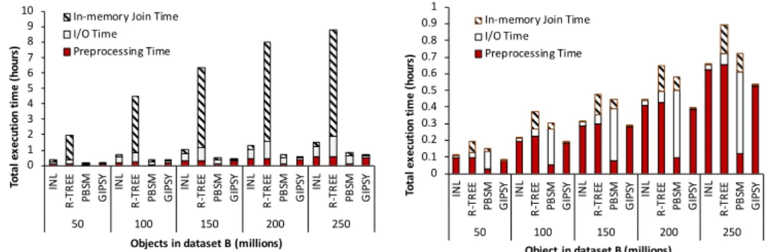
3.3.4 Visiting Order . . . 33 3.3.5 Start Point . . . 34 3.4 Experimental Evaluation. . . 35 3.4.1 Setup . . . 35 3.4.2 Experimental Methodology . . . 35 3.4.3 Combining Columns . . . 37 3.4.4 Building Mesocircuits . . . 39 3.4.5 Neuroscience Datasets. . . 41
3.4.6 GIPSY Sensitivity Analysis . . . 42
3.5 Conclusions . . . 44
4 Adapting to Spatial Datasets Characteristics 45 4.1 Introduction . . . 45 4.2 Motivation . . . 47 4.2.1 Motivating Experiment . . . 47 4.2.2 Motivating Application. . . 49 4.3 TRANSFORMERS Overview . . . 49 4.4 TRANSFORMERS Indexing . . . 51 4.5 TRANSFORMERS Join . . . 53 4.6 Transformations. . . 56 4.6.1 Role Transformation . . . 56
4.6.2 Data Layout Transformation . . . 57
4.6.3 Transformation Thresholds . . . 59
4.7 Experimental Evaluation. . . 60
4.7.1 Experimental Setup . . . 60
4.7.2 Experimental Methodology . . . 61
4.7.3 Robustness. . . 62
4.7.4 Non-uniform Data Distributions . . . 63
4.7.5 Uniform Data Distributions . . . 65
4.7.6 Neuroscience Data . . . 66
4.7.7 TRANSFORMERS Analysis . . . 66
Contents
II Workload-Aware Spatial Incremental Indexing 69
5 Disk-Based Incremental Indexing 71
5.1 Introduction . . . 71
5.2 Space Odyssey Overview. . . 72
5.3 Incremental Indexing. . . 73 5.3.1 Refinement Concept . . . 74 5.3.2 Optimizations . . . 75 5.4 Combining Datasets . . . 75 5.4.1 Merging Partitions . . . 76 5.4.2 Data Structures . . . 76 5.4.3 Querying . . . 77 5.4.4 Open Issues . . . 77 5.5 Experimental Evaluation. . . 78 5.5.1 Experimental Setup . . . 78 5.5.2 Experimental Analysis . . . 79 5.6 Conclusions . . . 83
6 In-Memory Incremental Indexing 85 6.1 Introduction . . . 85
6.2 Problem Definition . . . 87
6.3 Motivation . . . 88
6.3.1 Cracking for Spatial Data . . . 88
6.3.2 Disk-based Incremental Indexing in Main Memory . . . 89
6.4 QUASII Overview . . . 90
6.5 Data Structure & Query Processing. . . 93
6.5.1 Data Structure. . . 93
6.5.2 Query Processing and Index Refinement . . . 96
6.6 Experimental Evaluation. . . 99
6.6.1 Experimental Setup & Methodology . . . 99
6.6.2 Space-oriented Partitioning Challenges. . . 101
6.6.3 Incremental versus Static . . . 102
6.6.4 Comparative Analysis . . . 104 6.6.5 Analysis of QUASII . . . 107 6.6.6 Uniform Workload . . . 107 6.6.7 Performance Trends . . . 108 6.6.8 Impact of Selectivity . . . 108 6.7 Conclusions . . . 109
III Dictionary Compression Tailored for Spatial Data 111 7 Dictionary Compression in Point Cloud Data Management 113 7.1 Introduction . . . 113
7.2 Background . . . 115
7.2.1 Dictionary-based Compression. . . 115
7.2.2 Space-filling Curves . . . 117
7.3 Space-Filling Curve Dictionary-Based Compression . . . 118
7.3.1 Preprocessing & Data Structures . . . 120
7.3.2 Query Execution . . . 122
7.3.3 Space Requirements . . . 122
7.3.4 Impact of Space-filling Curve . . . 124
7.3.5 Scope . . . 128
7.4 Experimental Evaluation. . . 129
7.4.1 Space Requirements . . . 130
7.4.2 Query Performance. . . 132
7.4.3 Impact of Data Skew . . . 133
7.4.4 Impact of Selectivity . . . 134
7.4.5 Impact of Filtering . . . 134
7.4.6 Impact of Space-filling Curve: Time-efficiency. . . 135
7.4.7 Impact of Space-filling Curve: Space-efficiency . . . 136
7.4.8 Time- and Space-efficiency: Performance Trends . . . 137
7.4.9 Preprocessing cost . . . 138
7.4.10 Experimental Summary . . . 138
7.5 Conclusions . . . 139
8 Conclusions and Future Directions 141 8.1 Technological Impact. . . 141
8.2 Intellectual Impact . . . 142
Bibliography 160
List of Figures
2.1 Space-filling curves: Z-order and Hilbert curve. . . 10
3.1 Schema of a neuron’s morphology modelled with cylinders (left) and a visualiza-tion of a model microcircuit comprised of thousands of neurons (right). . . 25
3.2 Illustration of the use cases. . . 26
3.3 Total execution time as a result of joining uniform datasets of different densities. 27 3.4 GIPSY uses the sparse dataset to walk/crawl through the dense dataset.. . . 29
3.5 Partioning of the dataset with solid lines for the partitions and dashed lines for the elements MBRs.. . . 30
3.6 The data structures of GIPSY: summary pages, elements pages and pointers between them (arrows between summary records). . . 31
3.7 Starting with partition Q, GIPSY has to recursively visit all neighbors with inter-secting partition MBRs. . . 32
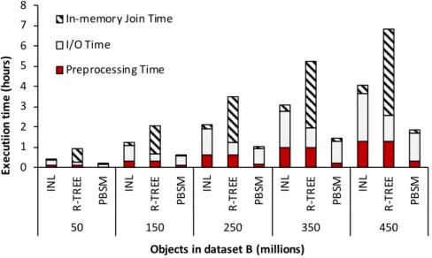
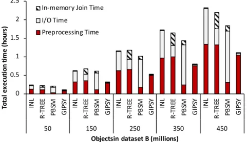
3.8 Total execution time as a result of one spatial join, combining columns.. . . 37
3.9 Number of I/Os as a result of one spatial join, combining columns. . . 38
3.10 Total execution time as a result of repeated join, combining columns. . . 38
3.11 Total execution time as a result of one spatial join, building mesocircuits.. . . . 39
3.12 Number of I/Os (logscale) as a result of one spatial join, building mesocircuits. 40 3.13 Total execution time as a result of repeated join, building mesocircuits. . . 40
3.14 Total execution time as a result of one spatial join for neuroscience datasets, combining columns (left) and building mesocircuits (right).. . . 41
3.15 Total execution time as a result of repeated join for neuroscience datasets, com-bining columns (left) and building mesocircuits (right). . . 41
3.16 Impact of sort strategies (left) and data distributions (right).. . . 42
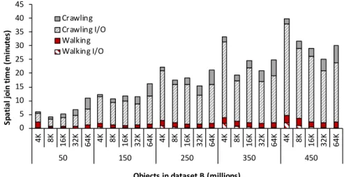
3.17 Spatial join time, varying the page size from 4KB to 64 KB. . . 43
4.1 Join time for datasets with variable relative density. . . 46
4.2 Illustration of variations in distribution and density. Each figure shows two datasets, one with grey elements and the other with black ones. . . 48
4.3 Neurocience data: axons (left) and dendrites (right). . . 49
4.4 TRANSFORMERS adapts to dataset characteristics. . . 51
4.5 The data structures: space node, space descriptor and space unit. . . 52
4.7 The hierarchical organization of TRANSFORMERS. . . 57
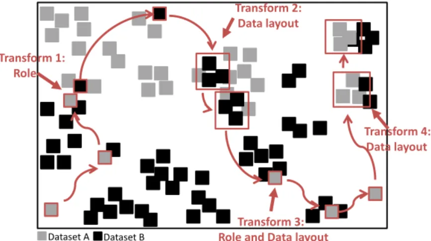
4.8 Role and Data layout transformation. . . 58
4.9 UniformCluster&DenseCluster(left) andMassiveCluster(right) dataset samples. 62 4.10 Joining datasets with variable relative density. . . 63
4.11 Execution time breakdown and number of intersection tests for the join phase on synthetic data. . . 64
4.12 Execution time breakdown and number of intersection tests for the join phase on neuroscience data. . . 66
4.13 Impact of transformations on join performance (left) and transformations thresh-old sensitivity (right).. . . 67
4.14 Adaptive exploration overhead. . . 68
5.1 Space Odyssey: components, data structures and a snapshot of the physical layout. 73 5.2 Incremental indexing strategy (in 2D).. . . 74
5.3 Query ranges: clustered, dataset ids: zipf. . . 80
5.4 Query ranges: clustered, dataset ids: heavy-hitter.. . . 80
5.5 Query ranges: clustered, dataset ids: self-similar. . . 80
5.6 Query ranges: uniform, dataset ids: uniform.. . . 81
5.7 Query times for each query in a sequence. . . 82
6.1 Overhead introduced when transforming query to the 1D space. . . 89
6.2 Incremental indexing strategy. . . 91
6.3 Index structure after the first (left) and few more (right) queries. . . 92
6.4 An example of query processing and incremental indexing in QUASII (configured withτx=4 andτy = 2), given ten spatial objects (o0–o9) and two range queries (q1andq2).. . . 94
6.5 Refinement step: query extension. . . 99
6.6 The impact of space-oriented partitioning. . . 101
6.7 Convergence of a) one-dimensional, b) space-oriented c) data-oriented based approaches. . . 103
6.8 Cumulative time of a) one-dimensional, b) space-oriented c) data-oriented based approaches. . . 103
6.9 Comparative analysis of incremental approaches: convergence. . . 105
6.10 Comparative analysis of incremental approaches: cumulative time. . . 106
6.11 Convergence and cumulative time: the first 500 (a & c) and last 100 (b & d) queries.107 6.12 Scalability analysis. . . 108
6.13 Impact of selectivity. . . 108
7.1 An example of range query execution over a dictionary-based representation of point cloud data. . . 116
7.2 Dictionary space, 2D illustration.. . . 118
7.3 SFC-DBC (data-aware) and SFC-based (space-oriented) partitioning strategy. . 119
List of Figures
7.5 The number ofSFCcodesexamined per query: the best and worst case. . . 125
7.6 Berlin aerial dataset, space requirements: a) total and b) breakdown. . . 131
7.7 AHN2 dataset: a) space requirements and b) query execution time (3D queries). 131 7.8 Berlin aerial dataset, query execution time: a) 3D and b) 2D range queries. . . 131
7.9 SFC-DBC: execution time breakdown.. . . 132
7.10 The impact of skew: space requirements and query execution time. . . 133
7.11 The impact of selectivity.. . . 134
7.12 The impact of filtering. . . 134
7.13 The impact of space-filling curve: query execution time for a) 125M and b) 500M points. . . 135
7.14 The impact of space-filling curve on space-efficiency. . . 136
7.15 SFC-DBC performance: a) query execution time and b) space requirements. . . 137
List of Tables
1
Introduction
We live in a data-driven era, with the opportunity to revolutionize science and enterprises by ex-tracting knowledge from massive amounts of data. Data-driven science exemplary showcases the power of data: scientific simulations have become a standard practice, complementing traditional methods for understanding natural phenomena across a number of scientific disciplines [36,41,46,48,82]. At the same time, enterprises harness the insights obtained through data analyses to improve existing services and offer new ones [25,51,56,135]. A significant percentage of the data collected and used has spatial properties, such as geomet-ric extent and location. Location Based Services (LBS) provide a set of functionalities based on geographical location, used by users on a daily basis. At the same time, LBS produce massive amounts of data associated with location. For instance, Uber announced 5 billion rides in 2017 [26], while Foursquare reached 12 billion check-ins [121]. Similarly, models used in scientific simulations across a number of domains (e.g., neuroscience, astronomy, and digital pathology) are typically represented with data that is enriched with spatial extent [41,46,82]. With technological advancements, the amount of spatial data will only continue to increase. Internet of Things (IoT) devices are one example – they are projected to reach 20 billion by 2020 [35] and are all equipped with location intelligence.
Spatial data management systems [42,77,105] are specifically designed to manage spatial data, considering its spatial property (i.e., location and extent) as a first-class citizen. Recent trends in data and applications, however, challenge the design of existing solutions. Data grows exponentially in volume, evolving in complexity alongside. At the same time, a number of emerging applications introduce new requirements that challenge current solutions.
1.1 Data Evolution
As a result of the recent technological improvement, spatial data has significantly evolved in recent years, increasing in volume and complexity.
Volume.Advances in data acquisition – through more powerful supercomputers for simula-tions, sensors with better resolusimula-tions, etc. – have caused an exponential growth in the volume of spatial data generated and collected. For instance, in the Human Brain Project (HBP) [82], neuroscientists build spatial models of a brain, consisting of millions of three-dimensional cylinders, where several thousand cylinders together reconstruct the spatial shape of a single neuron – the final brain model is expected to reach 1011neurons [127]. NASA released 500 TB of satellite earth observation data generated by remote sensing [87], while the Actueel Hoogtebestand Nederland 2 (AHN2) point cloud data set [88] contains 640 billion points acquired through airborne and terrestrial scanning. At the same time, people generate mas-sive amounts of volunteered geographic style information (VGI). This data is acquired either through community users of services such as OpenStreetMap [94] (a free editable map of the world, created by volunteers using local knowledge), or “unconsciously" – mostly through the use of smart phones (e.g., geo-tagged tweets, Facebook check-ins, etc.).
Complexity.Alongside with volume, spatial data has also increased in complexity [126]. By improving the precision of instruments and the granularity of the models, we also increase data density (the number of objects per space unit), non-uniformity (in terms of data distribution), and irregularity in geometric shapes. This trend is particularly evident in the scientific domain. In neuroscience simulations, for instance, a neuron’s morphology is modeled as a sequence of segments (cylinders) or through a fine-grain mesh representation [126,127]. Simulations can be performed at the cellular, sub-cellular or molecular level of detail [46]. Another example is pathology image analysis, where 3D micro-anatomic objects have complex structures and often non-uniform data distribution – e.g., the tissue affected by a tumor is significantly denser, in terms of its number of cells, compared to healthy regions [5]. The increase in data complexity is not limited to the scientific domain though. In OpenStreetMap, for instance, the densest areas have nearly three orders of magnitude more objects compared to the average [5].
1.2 Driving Applications
Technological advancements have triggered not just growth in data, but also in the number of emerging applications. These applications take spatial data as input, and often also produce spatial data as output, adding to the total amount of spatial data produced. Both traditional and new spatial applications are beneficial to the scientific and business domains, where a few examples include: 1) Scientific Simulations – simulations of spatial models have become a standard practice [6,41,41,82], complementing traditional methods for understanding natural phenomena across a number of scientific disciplines, 2) Digital Pathology – biomedical research is enhanced with the 3D exploration of micro-anatomic objects [71,72,73], 3) Urban Planning and Smart Cities – aerial scanning, combined with remote sensing technologies, enable planning and monitoring of the urban development process [1,23,31], and 4) Geo-graphic Information Systems (GIS) – systems designed to store and process geoGeo-graphic data naturally use massive amounts of spatial data and play an important role in natural resource and disaster management [32,119], telecommunication and network services [115], and more.
1.3. Data Management Challenges
As data volume and complexity increase, such applications become the main means that enable users to extract useful information from it. As such, these applications have potential to advance science and enterprises by enabling new discoveries, inspiring new products and improving existing services. The performance of such applications, and thus their useful-ness, is determined by their ability to process massive amounts of spatial dataefficiently. By efficiently, we refer to processing of data in atime-andspace-efficientmanner.
Time-efficiency. Given the massive volume of data, it has become imperative to use com-putational resources efficiently, i.e., to maximize performance and provide timely response. Applications have always wanted performance, however, as data size and complexity increase, this has become a critical requirement. For instance, Uber has to process user requests and provide services, such as dynamic pricing, in near real-time [27]. Urban planning applica-tions rely on visual analytics systems which are expected to provide interactive response times [23,139]. Finally, to advance scientific discovery, scientists rely on tools that enable fast processing of massive amounts of spatial data [46,47,52,123,126].
A number of applications focus on identifying and extracting useful insights from data, having the "usefulness criteria" defined at runtime. Their analysis is data-driven: users do not know a priory what they are looking for, and determine future steps based on the results of previous analyses. This new class of applications is described with a newly-coined term – data exploration [7,15,52,55,126]. Performing data exploration requires extracting knowledge from data in a timely manner [7,55,126]. More specifically, users need to analyze data the moment it is available. Otherwise, data could lose some or all of its value – which, by the time they discover it, might have already cost them significant time and processing resources. Space-efficiency. The increasing amount of stored and managed data demands for space-efficient data organization. Being space-space-efficient implies reduction in terms of resources necessary to store and transfer data. The primary motivation for the space-efficiency require-ment are the massive amounts of data that both scientific and enterprise applications have to store and manage today (Section1.1). To ensure resilience to errors, this data gets additionally replicated, increasing the total amount of data necessary to be maintained. Storage resources are cheap, however, their capacity cannot keep up with the exponential growth of data. There-fore, to handle this data deluge, we have to reduce space requirements and thus, the overall cost of systems. Alongside with storage reductions, space-efficient data organization has also the potential to improve performance [3,4,109,141].
1.3 Data Management Challenges
To meet the aforementioned requirements and fulfill their purpose, applications depend on efficient spatial analytics data management. Spatial data management has been an important research direction for more than four decades [33,42,77,105,112]. Traditionally, processing algorithms and supporting data structures have been designed specifically for spatial data to maximize performance benefits, taking into consideration its spatial property. Recent
technological advancements, however, make this insufficient and challenge the design of existing solutions and therefore, their ability to meet time- and space-efficiency requirements. Keeping Up with the Data Evolution.Increases in data volume and complexity challenge the time-efficiency and scalability of existing solutions. By becoming bigger, data gets also denser and more non-uniform with respect to data distribution, as discussed in Section1.1. Due to the changes in data properties, existing problems, which are common for spatial algorithms and data structures, get exacerbated, and new ones appear.
For instance, the overlap between nodes in data-oriented structures (i.e., the property of data-oriented partitioning, but also its challenge [33,113,130]) increases alongside with the increase in density – causing significant performance penalties [127]. Similarly, given the non-uniformity property, achieving robust performance with respect to the distribution of data is important in order to stabilize and optimize performance. The design of traditional data management solutions, however, is mostly agnostic to evolving data properties, i.e., it does not accommodate for these properties, incurring significant performance penalties [90,127,128]. Spatial join, a core operator in spatial analytics [58,76,78], is particularly affected by these changes, given its default high cost compared to the other types of spatial queries [76]. Supporting Ad-hoc Analysis. To conform with the data exploration requirements, we have to analyze data as soon as it is available, and to extract useful information quickly, in an ad-hoc manner. Traditional systems do not fulfill these requirements, as they require expensive preprocessing steps and a priori workload knowledge to meet the expected performance. Consequently, they significantly increase the data-to-insight time. Additionally, they can potentially waste both computational and storage resources, if the preprocessing cost is not amortized with the subsequent data analyses.
Addressing the aforementioned challenges, incremental and adaptive data processing forms the core of efficient data exploration [52,55]. To efficiently identify and extract useful infor-mation from massive amounts of data in an ad-hoc manner, algorithms and index structures have to be incremental, and adapt to the changes in data and workload seamlessly. While incremental and adaptive data processing have been extensively studied in the relational domain [7,45,52,53,54,55], they have been overlooked in the spatial domain, resulting in a lack of support for data exploration tasks. Traditional spatial data management systems require indexes to be built before analytical queries can be executed efficiently. Therefore, support for incremental indexing is key to efficient spatial analytics in an ad-hoc environment. Supporting Emerging Features.The evolving data properties and application requirements combined demand support for new features. Traditional solutions are not designed according to the emerging requirements and data properties, and therefore, cannot typically support new functionality efficiently – such that the data is used to its full potential and the demanding applications requirements are met. A driving force for new features is usually scientific discov-ery, where technological advancements and new use cases (novel methodologies) challenge the applicability of existing solutions [126,128]. Business applications are equally relevant,
1.4. Thesis Statement and Contributions
as they leverage new data sources to improve existing services or offer new products, where point cloud data management is a recent example [8,37,124,134].
With the advances in laser and image processing technology, data properties and users expec-tations in terms of point cloud management have evolved [124,134], challenging the efficiency of traditional file-based solutions. Data has increased significantly in size and precision. At the same time, applications want to use this data to its full potential: combining it with the other types of data, while using declarative and ad-hoc queries to explore it [8,124,134]. As a consequence, point cloud processing moved toward database management systems that are expected to provide both time- and space-efficiency, given the size of data.
1.4 Thesis Statement and Contributions
Spatial data analytics represent a powerful means to extract knowledge from data, however, due to recent technological advancements, there is a significant discrepancy between expecta-tions (determined by application requirements) and the actual ability of data management systems. The goal of this dissertation is to help advance spatial data management systems to reach their full and expected potential, by revisiting the design of traditional spatial data management systems and advocating for changes that will bridge the gap between the re-quirements and actual system performance.
Thesis Statement
Traditional spatial data management techniques underperform as the data size and complexity increase: they waste both computational and storage resources. Time- and space-efficiency of analytics is improved if spatial data management algorithms leverage and adapt to data characteristics and workload access patterns.
We revisit the design of spatial join algorithms, indexing techniques, and point cloud data management solutions based on the following key insights:
• Adapt to Data.Being agnostic to data characteristics and employing static strategies leads to sub-optimal, non-robust performance when joining datasets with non-uniform distribu-tions. The key to optimize performance is to be data-aware, that is to adapt the join strategy and supporting data structures to the underlying data distributions, in order to maximize performance and avoid wasting computational resources.
• Adapt to Workload.Workload-driven incremental index building significantly reduces the data-to-insight time. Indexes are built as a side-effect of query execution, and only for the parts of data queried, reducing computational and storage requirements. To ensure efficiency, incremental indexing should meet the following requirements: minimal data-to-insight time, efficient query performance, and low-cost incremental strategy.
• Leverage Data Characteristics.Preserving spatial proximity through data organization has the potential to improve time- and space-efficiency, as 1) data access patterns are frequently aligned with spatial proximity, i.e., objects close in space are frequently processed together, and 2) compression techniques can exploit spatial proximity. To maximize performance, it is equally important to leverage secondary data characteristics, other than spatial. These characteristics are typically introduced as a result of technological advancements and introduce new patterns in data that should be exploited.
Based on these insights, this dissertation makes the following technical contributions: • We present the design and implementation of two disk-based spatial join approaches that
leverage and adapt to dataset characteristics, achieving time-efficiency on non-uniform data distributions.
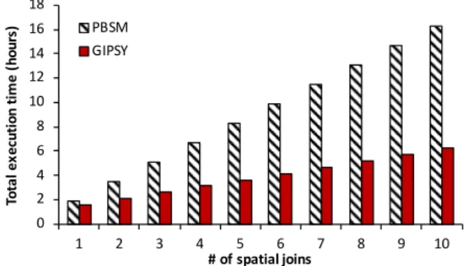
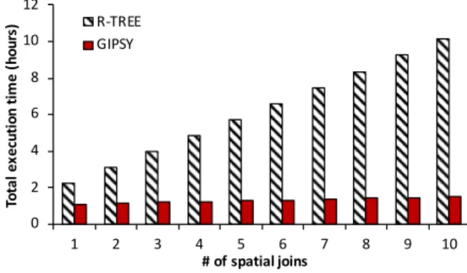
• GIPSY is a spatial join approach designed to efficiently join two datasets with contrasting densities. GIPSY uses the sparser dataset to guide the join process and therefore, by leveraging dataset characteristics, it selectively retrieves and joins only the data needed. GIPSY relies on data-oriented partitioning to produce fine-grain partitions, while avoiding overlap-related problems, by employing a crawling strategy.
• TRANSFORMERS achieves robust spatial joins on non-uniform data distributions, by adapting to dataset characteristics. We first show that the performance of the state-of-the-art spatial join approaches deteriorates when faced with variations in the distributions of data. To achieve robust performance and time-efficiency, TRANSFORMERS detects local variations in distributions and adapts the join strategy and data layout to local datasets characteristics at run-time.
• To achieve timely response and thus provide tools for efficient spatial data exploration, we design and develop two incremental indexing techniques. Both approaches take advantage of workload access patterns to significantly reduce data-to-insight time and achieve query performance comparable to traditional indexing approaches.
• Space Odyssey is designed for exploratory analyses of multiple spatial datasets that reside on disk. Without any prior information, Space Odyssey incrementally indexes the datasets and optimizes accesses to parts of the datasets frequently queried together, adapting their data layout on disk to the workload access patterns.
• QUASII is a query-aware spatial incremental index, designed for exploratory analyses of spatial data in main memory. It reduces data-to-insight time and curbs the cost of incremental indexing by gradually and partially sorting the data, while simultaneously producing a data-oriented hierarchical structure. In addition to QUASII, we also demon-strate the challenges of adapting and using existing incremental approaches (designed to incrementally index relational data) in the spatial domain.
• To accommodate for the recent requirements and adjust to evolving data properties, we present the design and implementation of a time- and space-efficient solution to storing and managing point cloud data in main memory column-store DBMS. We leverage point cloud
1.5. Thesis Organization
data properties, i.e., the frequent repetition of values for thex,y, andzcoordinates across point cloud entries, to employ dictionary-based compression in the spatial domain and thus achieve space-efficiency. To optimize for time-efficiency, we enhance dictionary-based compression with spatial indexing capabilities. More precisely, we integrate a space-filling curve order into the dictionary-based model, without requiring additional storage resources.
1.5 Thesis Organization
The rest of this thesis is organized as follows:
Chapter2presents related work and background information on the topics of this thesis. PartIpresents data-aware spatial joins, i.e., we introduce two spatial join approaches that leverage and adapt to dataset characteristics to achieve time-efficiency. Chapter3introduces GIPSY [99], a spatial join approach designed to efficiently join two datasets with contrasting densities. GIPSY uses the sparser dataset to navigate the join process and therefore, by lever-aging dataset characteristics, it selectively retrieves and joins only the data needed. Chapter4
presents TRANSFORMERS [100], a spatial join approach that achieves robust performance and time-efficiency on non-uniform data distributions by adapting to dataset characteristics. TRANSFORMERS detects local variations in distributions and adapts the join strategy and data layout to local datasets characteristics at run-time.
Incremental indexing enables timely response and saves both computational and storage resources by building an index as side-effect of query execution and indexing only the parts of the data queried. While incremental indexing has been extensively studied in relational domain, it has not been addressed in spatial data management. PartIIintroduces two query-aware incremental indexing approaches designed for exploratory analyses of spatial data. Chapter5presents Space Odyssey [101], designed for exploratory analyses of multiple spatial datasets that reside on disk. Space Odyssey takes advantage of workload access patterns to in-crementally index the datasets and optimize the access to datasets frequently queried together. Chapter6introduces QUASII [103], a query-aware spatial incremental index, designed for exploratory analyses of spatial data in main memory. To reduce data-to-insight time and curb the cost of incremental indexing, QUASII relies on a partial sorting strategy and data-oriented hierarchical structure.
PartIIIpresents a time- and space-efficient solution to storing and managing point cloud data in main memory column-store DBMS, motivated with the recent requirements and evolving data properties in point cloud data management. Our approach [102] (Chapter7) leverages point cloud data properties to employ dictionary-based compression in spatial domain and enhances it with indexing capabilities to achieve both time- and space-efficiency.
2
Background
In this chapter, we present a brief overview of topics that are related to this thesis, including a survey of related work. We begin by describing the key concepts in spatial data manage-ment. We then discuss traditional spatial access methods, designed for efficient querying of spatial data. We continue by giving an overview of the state-of-the-art in terms of spatial join techniques. Finally, we provide background on point cloud data management.
2.1 Fundamentals of Spatial Analytics
Spatial data management has been an important research direction for more than four decades [33,42,77,105,112]. Processing algorithms and supporting data structures have been designed specifically for spatial data, considering its spatial property as a first-class citizen. Two major properties that distinguish spatial from one-dimensional data and make its management challenging are: 1) a complex structure, and 2) its lack of total order. In the following we discuss in more detail these challenges and their implications [33,77,105]. We also address the general design behind spatial algorithms and supporting data structures and outline the common type of spatial queries.
2.1.1 Spatial Data Representation
The term spatial object has a broad sense – it can represent a point, line, polygon, spherical object, cube and more. Overall, we can categorize spatial objects into two categories: points and extended objects. A point is represented with its location in a two- or higher-dimensional space. Extended objects, such as lines, regions/polygons, or volumetric data (in 3D space), are also identified with a geometric extent that represents the geometric shape of the object. Therefore, a spatial object can represent a single point or a polygon defined by hundreds or thousands of points. Consequently, it is challenging to store, index, and process spatial data efficiently given its complex structure and varying size.
Figure 2.1 – Space-filling curves: Z-order and Hilbert curve.
To address the aforementioned challenge, spatial data is typically processed in two steps: filtering, followed by refinement [19,33,58]. In the filtering phase, algorithms work with approximations of the spatial objects. These approximations have significantly simpler struc-tures than the actual objects, and therefore they primarily minimize the computational cost. The goal of the filtering phase is to maximize the amount of data that can be processed using just the approximation geometry. This phase results in a candidate set – a list of objects that satisfy the spatial predicate given the approximation geometry. Finally, the refinement phase examines the actual objects from the candidate set to remove any false positives detected due to the use of approximation.
A typical object approximation is a minimum bounding rectangle (MBR) or a minimum bounding box (MBB), depending whether they represent 2D or 3D data. A MBB of an object is the smallest box that encloses the complete geometry of an object and it has iso-oriented sides. It is the most frequently used approximation because of its simple structure that minimizes computational and storage requirements. One of the issues associated with the approximation structures is the problem of dead space - a portion of space that is marked with the object’s approximation, but not occupied by the object. Several techniques [16,17] have been designed to minimize dead space in an object’s approximation and consequently improve the filtering stage. However, the overall benefit of these techniques might not be significant if they result in more complex structure that increases the storage requirements, the cost of pre-processing and the intersection tests.
2.1.2 Linear Orderings
One of the major challenges encountered when managing spatial data is the lack of a total order among spatial objects that preserves spatial proximity. More precisely, there is no total order that guarantees that any pair of objects which are close in the higher-dimensional space will also be close in the total order. Consequently, algorithms that use data sorting at their core cannot be directly employed for spatial data processing.
2.1. Fundamentals of Spatial Analytics
One way to introduce a notion of total order among spatial objects is by means of space-filling curves, such as the Z-order [96], the Hilbert curve [59], and the Gray-code curve [28]. A space-filling curve imposes a total, 1D order by visiting all the partitions in a D-dimensional grid exactly once, as illustrated in the Figure2.1. The order in which the partitions are visited defines their 1D codes and the order in 1D space. The granularity of the grid defines whether each object or group of objects will be assigned with a unique 1D code.
Given that it introduces the notion of total order, a space-filling curve also maps data to a one-dimensional domain, as it assigns 1D codes to spatial objects. Given such a mapping of spatial data, existing 1D access methods and algorithms can be used to manage spatial data. For instance, a B-Tree [11] can be used by transforming both data and queries in a 1D domain. It is important to note that the dimension reduction can introduce performance penalties. First, given that there is no natural total order among multi-dimensional objects, space-filling curves preserve spatial proximity up to different extents – depending on the employed ordering schema. Therefore, when mapping spatial data, it is crucial to consider space-filling curves that are effective in preserving spatial proximity [29,59,86], such as the Hilbert curve [59] and the Z-order [96]. Second, in order to achieve efficiency, the corresponding mapping schemes have to be adjusted not to introduce overheads with the transformation to 1D space. One example is range query mapping – if a simple mapping is considered, the transformed 1D range can be significantly larger than the original multi-dimensional range. Techniques that partition the curve into multiple sub-intervals, each of which is fully contained in the original range [132], address this issue.
2.1.3 Native Spatial Data Organization
Space-filling curves introduce the notion of total order, and consequently enable the use of 1D access methods and algorithms in spatial data management. While the dimension reduction provides simplicity, it also reduces the level of information and does not offer the same flexibility as the native, multi-dimensional domain. Therefore, a number of algorithms and data structures have been designed specifically for spatial data. One of their main design goals is to organize data such that spatial proximity is preserved. Preserving spatial proximity is important, as it has the potential to improve time- and space-efficiency, given that 1) data access patterns are frequently aligned with spatial proximity (i.e., objects close in space are frequently processed together), and 2) compression techniques can exploit spatial proximity. Considering the type of data partitioning (i.e., data organization) they employ, spatial algo-rithms and supporting data structures can be divided in two categories – approaches based on space- and data-oriented partitioning. The partitioning technique determines the benefits, but also the drawbacks for the corresponding family of approaches.
Space-oriented Partitioning.Space-oriented partitioning is done by partitioning the space containing the data, regardless of the spatial distribution of the objects [57,65,98,111]. The
produced partitions are disjoint, i.e., they do not overlap. Consequently, space-oriented partitioning entails a low-cost pre-processing step when it comes to identifying the partitions that contain the data of interests, as it typically employs a D-dimensional hash function. While space-oriented partitioning provides simplicity, it also limits the ability to adjust to the data distribution. More precisely, it does not provide explicit control over the number of elements assigned per partition and therefore, it can exhibit difficulties when handling skew. However, the major drawback of space-oriented partitioning is related to the handling of volumetric objects1. Given that the produced partitions do not overlap, a volumetric object can intersect with several partitions. To address this ambiguity, partitioning approaches use a multiple assignment or a multiple matching strategy.
The multiple assignment strategy assigns a copy of the object (or a reference) to each partition the object intersects with [89,98]. Doing so has the advantage that, given a point query, we can uniquely identify a partition that the query overlaps with or follow a single path while traversing a hierarchical data structure. Replicating objects, however, has several disadvantages: 1) results may be detected twice and deduplication is required or on-line duplicate removal [22], 2) the same object can be considered multiple times for the corresponding predicate check, 3) more data has to be stored and transferred, and 4) the grid configuration becomes more challenging as increasing the number of partitions also increases the replication rate.
The multiple matching strategy avoids replication of objects and assigns each object only to one partition it intersects with [9,65]. The corresponding data structure is equivalent to a hierarchy of space-oriented structures of increasing granularity. To partition the data, each object is assigned to the lowest level in the hierarchy, where it only overlaps with one partition. While this approach to partitioning avoids replication, it requires the inspection of multiple grids (that share a border).
Considering that the major drawback of space-oriented partitioning is related to the handling of volumetric objects, this type of data partitioning is mostly used to organize points, as they do not encounter similar issues. More precisely, while a volumetric object spans multiple disjoint partitions, a point is assigned to exactly one partition.
Data-oriented Partitioning.The data-oriented strategy partitions the data taking into consid-eration its spatial distribution [12,18,43,74]. The produced partitions consequently adjust to the data distribution, and control space utilization by limiting the number of objects assigned per partition. Adjusting to the data distribution is important, as it improves 1) handling skew in the data, and 2) data filtering capabilities – for instance, in the spatial join process we can use the partitions of one data set to build an index on the other dataset and/or to prune irrelevant elements. The control of space utilization is particularly useful for disk-based approaches, as it allows packing a fixed number of elements per partition.
2.1. Fundamentals of Spatial Analytics
The main design characteristics of data-oriented partitioning are that 1) an object is assigned to just one partition, and 2) partitions can overlap. Assigning an object to one partition eliminates problems related to multiple assignment and multiple matching strategies. Consequently, data-oriented partitioning is preferable when it comes to managing volumetric objects. However, assigning an object to just one partition in a data-oriented manner has also its drawbacks, as it results in overlaps among partitions that can degrade performance. More precisely, given a point query, we cannot uniquely identify the partition that the query overlaps with or follow a single path while traversing a hierarchical data structure. To address the problem of overlap, several approaches partition the data by producing non-overlapping regions. However, to be able to achieve so, they allow object replication and consequently encounter similar problems to space-oriented partitioning approaches.
2.1.4 Spatial Queries
A number of approaches have been designed to address efficient spatial query execution. In the following we outline the common query types used for spatial data analyses.
• Range Query.A range query is the most common type of spatial query. Given a datasetA, a spatial regionr(or a reference objecto), and a predicateθ, it retrieves all the objects from the datasetAthat satisfy the spatial predicateθwith respect to the regionr(or a reference objecto) [33,77]. The spatial predicate can be defined with any spatial relationship between objects, such as intersection, enclosure, or containment. The region can be explicitly defined (typically as an iso-oriented region), or inferred based on the reference object. For instance, by using a range query we can inspect the properties of a spatial model given a specific region in the space, or find all hotels within 500 meters from a user’s current location. • Nearest Neighbor Query. Given a datasetA and an objecto, a nearest neighbor query
returns all the objects from datasetAthat have the minimum distance from the objecto. Formally defined,N NQ(o)={a∈A:∀a0∈A,d i st(a,o)≤d i st(a0,o)} [33,77]. One variant of the nearest neighbor query is the k-nearest neighbor query that returns the k nearest neighbors. For instance, finding the 5 restaurants closest to a user’s location.
• Spatial Join Query. Given two datasets of spatial objects A andB, and a predicateθ, a spatial join query returns the pairs of objects that satisfy the spatial predicate. Formally, A./θ B ={(a,b) :a ∈ A,b ∈B,aθb}. The efficient execution of spatial join queries is important in many different applications. In scientific applications, for example, spatial joins are used to determine the location of synapses in brain models, in medical imaging to determine the proximity of cells, and in geographical information systems spatial joins detect collisions between geographical features like houses, roads, etc.
2.2 Spatial Indexing
Research in indexing spatial data has produced numerous approaches for the fast and scalable querying of spatial datasets [33]. We first discuss the traditional approach to indexing, where an index is built as part of pre-processing. We then introduce the concept of incremental indexing and related approaches.
2.2.1 Traditional Indexing
We briefly review traditional spatial indexing approaches that we group into two classes according to the division introduced in Section2.1.3. Each class inherits the benefit and drawbacks characteristic of the corresponding family of approaches. We do not distinguish between methods for points and volumetric objects. The approaches that are designed for points can be adopted to handle volumetric objects using the query extension technique [122]. The basic concept is to represent a volumetric object by its center, and use a query enlarged by the size of the biggest object [122]. However, as discussed in Section2.1.3, approaches based on space-oriented partitioning are typically used to manage point data, while data-oriented partitioning is a preferable choice for volumetric objects.
Space-oriented Indexing. A typical representative of approaches based on space-oriented partitioning is the uniform grid that partitions the space uniformly into partitions of equal size [114,116], employing the multiple assignment strategy. Similarly, the Quadtree [111] and its variant for 3D space, the Octree [57], recursively divide space into four/eight partitions of equal size to build a hierarchy of partitions.
Further approaches, for example the grid file [89], use a non-uniform grid to better accommo-date skew in the data (and to optimize for disk accesses). The downside is a more complex query execution, due to cells of different sizes and locations. The two level grid file [49] ad-dresses the issue by introducing an additional level with a coarser grid. Still, the overhead of testing a query against multiple cells can be substantial. Further work improves on the space utilization by adding a second grid [50]. BLOCK [92] is a recent in-memory index designed to reduce the number of intersection tests by adjusting the granularity of the grid to the spatial properties of the query. To achieve this, it creates a set of grids of different granularity, and splits each query across the available grids.
A space-filling curve [28,59,96] uses space-oriented partitioning at its core. More precisely, the corresponding curve is constructed by ordering the cells of a uniform grid. Given that the space-filling curve transforms spatial data from a multi- to a one-dimensional domain, existing 1D access methods, such as the B-Tree [11], can be used for querying.
Data-oriented Indexing.The R-Tree [43], arguably the most important data-oriented spatial index, is a multi-dimensional generalization of the B-Tree, which recursively encloses objects in MBRs. The basic R-Tree definition faces the problems of overlap and dead space, both
2.2. Spatial Indexing
detrimental to query execution performance [43,127]. Multiple approaches have been devised to address the issue. The R*-Tree [12], for example, uses an improved version of the node split algorithm and reinsertion of objects, while the R+-Tree [113] tries to avoid overlap through the duplication of MBRs. A priori knowledge of the entire dataset may help to reduce the above problems of the R-Tree by packing spatially close objects on the same disk page. The Hilbert R-Tree [61] achieves this using the Hilbert curve, Sort-Tile-Recursive (STR) [70] recursively sorts objects in all dimensions to do so, while Top-down Greedy Split (TGS) [34] recursively splits the data set into partitions, minimizing the area on each level.
Adaptive index structures [125] are designed to optimize disk-access for data-oriented indexes (including the R-Tree index), based on the query workload. The core idea is to rearrange the index nodes in response to queries, so that they can be accessed sequentially on disk. While most of the R-Tree-based indexes are designed for disks, the CR-Tree [64] optimizes R-Trees for main memory access. The CR-Tree is a cache-conscious version of R-Tree. To reduce the number of cache misses in R-Tree, CR-Tree proposes a MBR compression scheme that reduces the index size and enables the alignment of the nodes to the cache lines.
The KD-Tree [13] is a binary search tree that recursively divides space, using an iso-oriented hyperplane to divide the space into two parts at every step. The adaptive KD-tree [14] extends the initial KD-Tree design. It takes into account data distribution by splitting the space into two partitions, such that each partition contains approximately the same number of points. While the KD-Tree is designed for points, the SKD-tree [93] or spatial KD-Tree is designed for volumetric objects.
2.2.2 Incremental Indexing
Traditional systems require indexes to be built before analytic queries can be executed effi-ciently. More precisely, they require sufficient idle time for an index to be build before any kind of analyses can be performed. Modern, data-driven applications, however, do not conform to these requirements. Their goal is to analyze data as soon as it is available, i.e., to minimize data-to-insight time.
The concept of incremental indexing addresses this challenge: to reduce data-to-insight time, an index is built as a side-effect of query execution and only for the parts of the data queried. To the best of our knowledge, no incremental strategy has been proposed for spatial indexing. Nevertheless, there has been considerable interest in incremental data processing within relational databases. We thus briefly describe approaches used by relational database systems. Incremental indexing techniques have been extensively studied in database cracking [45,
53,54] and adaptive merging [38,39]. Both categories of techniques distribute the cost of sorting across the queries. The former partially sorts keys in an in-memory relation, essentially performing quicksort. The latter, adaptive merging, takes the idea further and devises an
incremental, external sort to make use of external memory as well. Similarly, incremental approaches can be used to index time-series [140].
Driven by the same goal, novel systems have been proposed that bypass the data pre-processing step and execute queries on raw data files. Instead, auxiliary data structures are built incrementally so that the most popular data subsets are serviced at the speeds of fully loaded/indexed data. For example, NoDB [7], RAW [62], and ViDa [63] incrementally build positional maps to track the position of frequently accessed data fields. This enables these systems to “jump” to previously queried data regions and potentially reduce the costs of tokenizing and parsing raw data sources. Following the same paradigm, Slalom [91], an in-situ query engine, provides on-the-fly partitioning and indexing schemes based on the information collected by lightweight monitoring.
2.3 Spatial Joins
Spatial join is one of the fundamental operators in spatial analytics [58,76,80,131]. Given two datasets of spatial objects, a pairwise spatial join finds the pairs of objects that satisfy the spatial predicate. The predicate can be defined with any spatial relationship between objects, such as intersection, enclosure, or distance – where intersection/overlap is the most commonly used. Given its importance, a number of algorithms have been developed to perform spatial joins, where the majority is designed for disk. Following the division introduced in Section2.1.3, we categorize the approaches according to the use of space- or data-partitioning strategies. Space-oriented Partitioning.We organize join methods based on space-oriented partitioning into two groups according to the use of a multiple assignment or multiple matching strategy. PBSM [98], the partition based spatial-merge join, partitions the space uniformly into cells of equal size, employing the multiple assignment strategy. In the first phase, each element of both datasets is assigned/replicated to all cells it overlaps with. In the second phase, PBSM iterates over all cellsc∈Cand tests all elements of datasetAincagainst all elements of dataset Bincto find pairwise intersections.
The size separation spatial join (S3) [65] uses a hierarchy of equi-width grids of increasing granularity. Each element of both datasets is assigned to the lowest level in the hierarchy where it only overlaps with one cell. To perform the join, S3 iterates over each cellcin the hierarchy and joins it with all cells that covercon a higher level, following the concepts of the multiple matching strategy.
The scalable sweeping-based spatial join [9], a representative of the multiple matching strategy, partitions the space intonstrips of equal width in one dimension and assigns each element e of both datasets to the strip wheree is fully contained. In each of then strips it uses a plane-sweep approach to determine all intersections between elements of datasetsAandB.
2.4. Point Cloud Data Management
Elements intersecting with several strips (e.g., from stripito stripk) are assigned to setSi k.
When swiping stripjall setsSj k withj<n<kare also joined.
Data-oriented Partitioning.We organize joins based on data-oriented partitioning into three categories, depending on whether they require an index on none, one, or both datasets. The synchronized R-Tree traversal [18] synchronously traverses the R-Trees [43]RAandRB
built based on datasets A andB. Starting at the root nodes ofRA andRB, the approach
traverses the trees top down and, if two nodesnA∈RAandnB∈RBon the same level intersect,
recursively tests their children. On the bottom level, the spatial elements are tested for intersection. Optimization techniques, such as search space restriction, or sorting based on the plane sweep strategy [18], can be used to reduce the cost of intersection tests.
While the synchronized R-Tree traversal requires both datasets to be indexed, the indexed nested loop join [24] only requires an indexIA on datasetA. It iterates over datasetBand
queriesIAfor each elementb∈Bwithbas the query. The query results are all intersections of
binA. Given the considerable cost of a query, this approach is only efficient in caseA>>B. Several approaches take advantage of existing indexes by using seed-style strategies. The seeded tree approach [74] assumes the existence of an R-Tree indexIAbuilt based on dataset
A. It usesIAas a template to build a second R-Tree indexIBbased on datasetB. Both indexes
are joined with the synchronous R-Tree traversal [18] approach. AsIB is built based onIA, the
bounding boxes are aligned leading to less overlap and the synchronous join therefore has to compare fewer bounding boxes. The slot index spatial join [79] uses the existing R-Tree index IAas partitioned data, i.e., to define a set of partitions or slots. The slots are used to partition
the non-indexed datasetB, applying simultaneously data filtering – the objects that do not intersect with any slot are filtered. In the final phase, the corresponding partitions are joined. The spatial hash join [75] similarly applies the seed-style strategy, however, it does not assume the existence of indexes. It uses sampling to hash dataset A into a predefined number of buckets. The produced buckets are then used as a seed to partition datasetB. While the seed strategy enables data filtering, it also produces partitions that might not be reused given that parts of datasetBare filtered out.
2.4 Point Cloud Data Management
Point cloud data is a useful source of information for natural resource management, urban planning, architecture and more. It represents a set of 3D points used to model an object or area, exploiting a number of properties such asx,y, andzcoordinates, angle of scan, and color. We first give a general overview of existing point cloud management systems, following up with compression and indexing capabilities of current systems.
General.File-based solutions (e.g., LAStools [108]) represent a traditional approach to point cloud data management: points are stored in files in a predefined format and processed by