Forecasting. Forecasting Application. Practical Forecasting. Chapter 7 OVERVIEW KEY CONCEPTS. Chapter 7. Chapter 7

(1)

1

Forecasting

Chapter 7 Chapter 7 2

Chapter 7

OVERVIEW

Forecasting Applications Qualitative Analysis

Trend Analysis and Projection

Business Cycle

Exponential Smoothing

Econometric Forecasting

Judging Forecast Reliability

Choosing the Best Forecast Technique

3

Chapter 7

KEY CONCEPTS

macroeconomic forecasting microeconomic forecasting qualitative analysis personal insight panel consensus delphi method survey techniques trend analysis secular trend cyclical fluctuation seasonality

irregular or random influences linear trend analysis growth trend analysis business cycle economic indicators composite index economic recession economic expansion exponential smoothing one-parameter (simple) exponential

smoothing

two-parameter (Holt) exponential smoothing

three-parameter (Winters) exponential smoothing econometric methods identities behavioral equations forecast reliability test group forecast group sample mean forecast error

4

Forecasting Application

Macroeconomic Applications

Predictions of economic activity at the national or

international level.

Microeconomic Applications

Predictions of company and industry performance.

Forecast Techniques

Qualitative analysis.

Trend analysis and projection. Exponential smoothing. Econometric methods.

5

“

Practical

”

Forecasting

6

POS and syndicated data measure consumer

purchases from a retail outlet.

MANUFACTURER MANUFACTURER SHIPMENTS SHIPMENTS CONSUMER CONSUMER TAKEAWAY TAKEAWAY CUSTOMER CUSTOMER WAREHOUSE WAREHOUSE RETAIL STORE

RETAIL STORE SHOPPING SHOPPING

HOUSEHOLD HOUSEHOLD CUSTOMER CUSTOMER ORDERS ORDERS CUSTOMER CUSTOMER HQ/BUYER HQ/BUYER aka aka CONSUMPTION CONSUMPTION SELL SELL--THROUGHTHROUGH

(2)

7

Although both measure the same thing, Although both measure the same thing, there are some key differences between POS and there are some key differences between POS and

syndicated data. syndicated data.

POS (point-of-sale)

POS

(point-of-sale) SyndicatedSyndicated(scanner)_(scanner)

Who supplies it Measures available Channels available Coverage Delivery lag time Processing required

Retailer 3rdparty vendors (IRI, ACNielsen, etc.) Volume, (pricing) Volume, pricing, distribution,

merchandising

Individual retailer Grocery, Drug, Club, C-Store, Mass Merch (excl. Wal*Mart)

All stores Some census, some projected from sample Varies (1 day – monthly) 10 days – monthly (can often pay for

faster for some channels) Wide variation Minimal

8

How is syndicated data collected?

Volume

Volume Feature AdsFeature Ads DisplaysDisplays Price Price Distribution Distribution SOURCES Retailer POS System (dollar sales, unit sales)

Retailer

POS System

POS System (dollar sales, unit sales)

(dollar sales, unit sales) Ad Ad Ad “clearing _house_house“_house”“clearing clearing _”_” InInIn-store auditors--store auditorsstore auditors

more accurate less

11

Qualitative Analysis

Expert Opinion

Informed personal insight is always useful.

Panel consensus reconciles different views.

Delphi method seeks informed consensus.

Survey Techniques

Random samples give population profile.

Stratified samples give detailed profiles of

population segments.

12

Trend Analysis and Projection

Trends in Economic Data

Secular trends reflect growth and decline.

Cyclical fluctuations show rhythmic variation.

Seasonal variation (weather, custom).

Random influences are unpredictable.

13

Linear Trend Analysis

Assumes Constant Period

-

by

-

Period

Change

Illustrated in Figure 7.2 on Page 202

bXt

a

S

_t

=

+

See Table 7.1 Data, Pg. 203 See Table 7.1 Data, Pg. 203

See page 200 See page 200

14

Growth Trend Analysis

Comes in two versionsComes in two versions

Constant Rate of GrowthConstant Rate of Growth

Continuous (as opposed to annual) Continuous (as opposed to annual)

Compounding Compounding

(3)

15

Constant Annual Rate of Growth

Estimated by using a Estimated by using a ““semisemi--log transform.log transform.””

Take the log of the dependent variable to Take the log of the dependent variable to

the base 10 the base 10

Assumes Assumes AnnualAnnualcompoundingcompounding

See page 203/4 See page 203/4

16

Continuous Compounding Rate of

Growth

Estimated using the Estimated using the ““semisemi--log transform.log transform.””

Take the natural log of the dependent Take the natural log of the dependent

variable (i.e., to the base e). variable (i.e., to the base e).

Assumes Assumes ContinuousContinuous(not annual) (not annual)

compounding compounding

See page 204/5 See page 204/5

17

Linear Trend Analysis

Growth Trend Analysis

Linear and Growth Trend Comparison

18 Figure 7.2

19

Figure 7.1

(4)

21

Business Cycle

What Is the Business Cycle?

Rhythmic pattern of economic expansion and

contraction.

Economic Indicators

Useful leading, coincident and lagging

indicators help forecasters. Economic Recessions

Periods of declining economic activity.

Sources of Forecast Information

22

Figure 7.3

23

Indicators

(Business Cycle Indicators)

Developed by NBERDeveloped by NBER

Indicators are related to turning points in Indicators are related to turning points in

business cycles business cycles

Business Cycle defined as "expansions Business Cycle defined as "expansions

occurring at about the same time in many occurring at about the same time in many economic activities" economic activities" See Pg. 207 See Pg. 207 24

Indicators continued

Leading IndicatorsLeading Indicators

--lead turning pointslead turning points

Coincident IndicatorsCoincident Indicators

--are coincident with turning pointsare coincident with turning points

Lagging IndicatorsLagging Indicators

--lag turning pointslag turning points

Turning points are the key to forecasting Turning points are the key to forecasting

with indicators. with indicators. 25

Indicators

Level of Economic Activity Time <- Period -> 26 Composite Indexes of 10 Leading, Four Coincident, and Seven Lagging Indicators (1987 + 100) Composite Composite Indexes of Indexes of 10 Leading, 10 Leading, Four Four Coincident, Coincident, and Seven and Seven Lagging Lagging Indicators Indicators (1987 + 100) (1987 + 100)

(5)

27

Composite Indicators

Index of Index of LeadingLeadingIndicators Indicators

Currently includes 10 indicators:Currently includes 10 indicators:

Average Workweek; Initial Claims Unemployment; Average Workweek; Initial Claims Unemployment; New Orders Consumer Goods;

New Orders Consumer Goods;

Vendor Performance; New Orders Capital Goods; Vendor Performance; New Orders Capital Goods; Building Permits; Stock Prices; M2;

Building Permits; Stock Prices; M2;

Interest Rate Spread; Index of Consumer Expectations Interest Rate Spread; Index of Consumer Expectations

(See www.tcb-indicators.org) See Page 209_{See Page 209}

28

Composite Indicators

Index of

Index of CoincidentCoincidentIndicators Indicators Currently includes 4 indicators: Currently includes 4 indicators:

Employees in nonagricultural payrolls;Employees in nonagricultural payrolls;

Industrial production index;Industrial production index;

Personal income less transfer payments;Personal income less transfer payments;

Manufacturing and trade sales.Manufacturing and trade sales.

(See www.tcb-indicators.org) See Page 209See Page 209

29

Index of

Index of LaggingLaggingIndicators Indicators Currently includes 7 indicators: Currently includes 7 indicators:

Change in labor cost;Change in labor cost;

Ratio of inventories to sales;Ratio of inventories to sales;

Average duration of unemployment;Average duration of unemployment;

Ratio consumer installment credit to personal Ratio consumer installment credit to personal

income; income;

Commercial and industrial loans;Commercial and industrial loans;

Prime rate;Prime rate;

Change in CPI for services.Change in CPI for services.

(See www.tcb-indicators.org)

See Page 209 See Page 209

30

Exponential Smoothing

One-parameter Exponential Smoothing

Used to forecast relatively stable activity.

Two-parameter Exponential Smoothing

Used to forecast relatively stable growth.

Three-parameter Exponential Smoothing

Used to forecast irregular growth.

Practical Use of Exponential Smoothing

Techniques

31 Figure 7.4 32

Simple Exponential Smoothing

The simple exponential smoothing model can be written in the following manner:

Ft+1=wAt+

(

1−w

)

Ft

Ft+1=forecasted value for next period

w=The smoothing constant 0

(

<a<1

)

At=Actual value of time series now (in period t)

Ft=Forecasted value for time t

See Pg. 215

(6)

33

Time

Time CalculationCalculation Weight for Weight for XX_t_t t t .1.1 t t--11 .9 X .1.9 X .1 .090.090

α

= .1

tt--22 .9 X .9 X .1.9 X .9 X .1 .081.081 t t--33 .9 X .9 X .9 X .1.9 X .9 X .9 X .1 .073.073 . . . . . . ---Total = Total = 1.0001.000

Alpha Factor in Smoothing

34

Time

Time CalculationCalculation Weight for Weight for XX_t_t t t .9.9 t t--11 .1 X .9.1 X .9 .09.09

α

=.9

tt--22 .1 X .1 X .9.1 X .1 X .9 .009.009 t t--33 .1 X .1 X .1 X .9.1 X .1 X .1 X .9 .0009.0009 . . . . . . ---Total = Total = 1.0001.000

Alpha Factor in Smoothing

35

Root Mean Square Error

Root Mean Square Error is used to evaluate the relative accuracy of various forecasting methods; it is easy for most people to interpret because of similarity to the basic statistical concept of a standard deviation.

RMSE

=

A

t

−

F

t

(

)

2 t=1 n

∑

n

36

Calculating Root Mean Square

Error

Calculate the sum of the squared Calculate the sum of the squared

errors: errors:

Calculate the mean squared error:Calculate the mean squared error:

A

t

−

F

t

(

)

2 t=1 n

∑

A

t

−

F

t

(

)

2 t=1 n

∑

n

37

Calculation continued

Finally, take the square root of the Finally, take the square root of the

mean sum of squared errors: mean sum of squared errors:

The smaller the RMSE, the "better" the The smaller the RMSE, the "better" the

forecast model. forecast model.

RMSE can be used to evaluate any RMSE can be used to evaluate any

forecasting model. forecasting model.

RMSE

=

A

t

−

F

t

(

)

2 t=1 n

∑

n

38

Smoothing Rule of Thumb

In actual practice, alpha values from 0.05 to 0.30 work very well in most simple smoothing models.

If a value of greater than 0.30 gives the best RMSE this usually indicates that another forecasting technique would work even better.

(7)

39

Pros and Cons of Smoothing

Pros:

• Requires a limited amount of data

Cons:

40

Pros and Cons of Smoothing

Pros:

• Relatively simple compared to other forecasting methods

Cons:

41

Pros:

Cons:

• Its forecasts lag behind actual data

42

Pros and Cons of Smoothing

(See Unemployment and Gapsales) Pros:

Cons:

• Its forecasts lag behind actual data • No adjustment for trend or seasonality

43

Holts Exponential Smoothing

Used for data exhibiting some trend over Used for data exhibiting some trend over

time time

Is just as simple to apply as simple Is just as simple to apply as simple

smoothing smoothing

(See Unemployment and Gapsales)

See Pg. 215

44

Winters Exponential Smoothing

Adjusts for both trend and seasonalityAdjusts for both trend and seasonality

Is just as simple to apply as simple Is just as simple to apply as simple

smoothing smoothing

Involves the use of 3 smoothing Involves the use of 3 smoothing

parameters, simple smoothing parameter, parameters, simple smoothing parameter, trend smoothing parameter, and

trend smoothing parameter, and seasonality smoothing parameter seasonality smoothing parameter (See Unemployment and Gapsales)

See Pg. 215

(8)

45

Advantages of Econometric Methods

Models can benefit from economic insight.

Forecast error insight can improve models.

Single Equation Models

Show how Y depends on X variables.

Multiple-equation Systems

Show how many Y variables depend on X

variables.

46

Judging Forecast Reliability

Tests of Predictive Capability

Consistency between test and forecast sample

suggest predictive accuracy. Correlation Analysis

High correlation suggests predictive accuracy.

Sample Mean Forecast Error Analysis

Low average forecast error suggests

predictive accuracy.

47

Econometric Forecasting

Large Scale Macroeconomic ModelsLarge Scale Macroeconomic Models

Smaller Scale Industry ModelsSmaller Scale Industry Models

Individual Product Demand ModelsIndividual Product Demand Models

See Page 218 See Page 218

48

Large Scale Macroeconomic Model

(with only 4 equations)

Behavorial Equation (Consumption):

C = a+b (GNP)

Behavorial Equations (I and G): I = 400

G = 500 Identity:

GNP = C + I + G

See page 219 Multiple Equation Systems See page 219 Multiple Equation Systems

49

Large Scale Macroeconomic Model

(with only 4 equations)

Substitute consumption equation into identity:

Solve for GNP:

Substitute regression estimates into model:

GNP= 1 1−b ⎛ ⎝ ⎞ ⎠

(

a+I0+G0

)

GNP=a+b(GNP)+I0+G0 GNP= 1 1−.72 ⎛ ⎝ ⎞ ⎠ −

(

266.1+400+500

)

50

Evaluating the Model

GNP= 1

1−.72

⎛

⎝ ⎞ ⎠ −

(

266.1+400+500

)

GNP =2, 263. 657

When new values of Investment and government expenditures become available, the model may be evaluated again. New parameters are determined frequently.

(See the “Fairmodel” at http://fairmodel.econ.yale.edu/)

(9)

51

Choosing the Best Forecast

Technique

Data Requirements

Scarce data mandates use of simple forecast

methods.

Complex methods require extensive data.

Time Horizon Problems

Short-run versus long-run.

Role of Judgment

Everybody forecasts.

Better forecasts are useful.

52

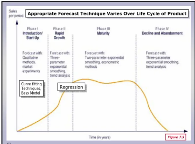
Appropriate Forecast Technique Varies Over Life Cycle of Product

Appropriate Forecast Technique Varies Over Life Cycle of Product

Figure 7.5 Curve fitting Techniques, Bass Model Curve fitting Techniques,

Bass Model Regression

Regression

71

Regression Models in Forecasting continued Regression Models in Forecasting continued

Accounting for SeasonalityAccounting for Seasonality

Extensions of Multiple RegressionExtensions of Multiple Regression

Forecasting Domestic Car SalesForecasting Domestic Car Sales