Alma Mater Studiorum
Università di Bologna
DOTTORATO DI RICERCA IN SCIENZE STATISTICHE CICLO XXX Settore Concorsuale: 13/D1 Settore Scientico Disciplinare: SECS-S/01Solution Path Clustering for
Fixed-Eects Models in a Latent
Variable Context
Presentata da: Francesco Giovinazzi
Coordinatore Dottorato:
Supervisore:
Prof.ssa Alessandra Luati
Prof.ssa Silvia Cagnone
Co-supervisore:
Prof. Francesco Bartolucci
Abstract
The main drawback of estimating latent variable models with xed eects is the direct dependence between the number of free parameters and the number of observations. We propose to apply a well suited penalization technique in order to regularize the parameter estimates. In particular, we promote sparsity based on the pairwise dierences of subject-specic param-eters, inducing the latter to shrink on each other. This method allows to group statistical units into clusters that are homogeneous with respect to a latent attribute, without the need to specify any distributional assumption, and without adopting random eects. In practice, applying the proposed pe-nalization, the number of free parameters is reduced and the adopted model becomes more parsimonious. The estimation of the xed eects is based on an algorithm that builds a solution path, in the form of a hierarchical ag-gregation tree, whose outcome depends on a single tuning parameter. The method is intended to be general, and in principle it can be applied on the likelihood of any latent variable model with xed eects. We describe in detail its application to the Rasch model, for which we provide a real data example and a simulation study. We then extend the method to the case of a latent variable model for continuous data, where the number of xed eects to be estimated is higher.
Contents
1 Introduction 1
2 Fixed-Eects Latent Variable Models 9
2.1 Latent Variables as Fixed or Random Eects . . . 9
2.2 The Rasch Model . . . 11
2.2.1 Notation . . . 11
2.2.2 The model . . . 11
2.2.3 Fixed Eects or Random Eects . . . 14
2.2.4 Estimation with the Joint Maximum Likelihood . . . . 15
2.2.5 Latent Class Rasch Model . . . 18
2.2.6 Limits of the JML . . . 18
3 An Overview on Lasso-Type Penalties 21 3.1 The Lasso . . . 21
3.1.1 Notation . . . 21
3.1.2 The Lasso for Linear Regression . . . 22
3.1.3 The Lasso for Logistic Regression . . . 26
3.1.4 Inference and Cross-Validation . . . 26
3.2 Generalizations of the Lasso . . . 27
3.2.1 The Elastic Net . . . 28
3.2.2 The Group Lasso . . . 29
3.2.3 The Fused Lasso . . . 30
3.2.4 The Pairwise Fused Lasso . . . 31
3.3 Lasso-Type Penalties for Clustering . . . 32
3.3.1 The Solution Path Clustering . . . 33
4 A Penalized Fixed-Eects Rasch Model for Clustered Abili-ties 37 4.1 The Penalized Fixed-Eects Rasch Model . . . 37
4.1.1 Denition of the Optimization Problem . . . 37
4.1.2 The SPC algorithm . . . 42
4.3 Real Data Example: INVALSI data . . . 48
4.4 Simulation Study . . . 55
5 A Penalized Fixed-Eects Model for Continuous Responses with Clustered Eects 63 5.1 The Penalized Fixed-Eects Model for Continuous Responses . 63 5.1.1 Denition of the Optimization Problem . . . 64
5.1.2 The SPC algorithm . . . 66
5.2 Real Data Example . . . 68
5.3 Simulation Study . . . 71
6 Final Remarks 79
Appendix 83
List of Figures
2.1 Item characteristic curves of a Rasch model for 5 items with
increasing diculty levels. . . 13
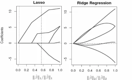
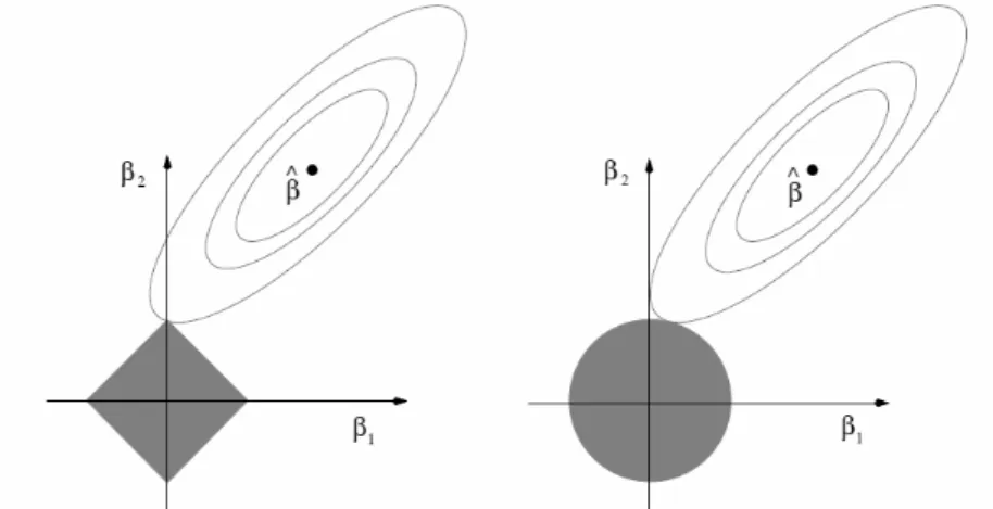
3.1 Solution paths for the lasso (left) and ridge regression (right). 24 3.2 Geometrical interpretation of the lasso (left) and ridge regres-sion (right) with J = 2. . . 25
3.3 Constraint regions for a penalty of the general formPJ j=1|βj| q with dierent values ofq. . . 25
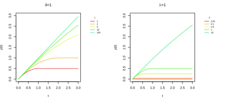
3.4 Geometrical study of the MCP penalty for growing values of λ and δ keeping the other xed to 1. . . 34
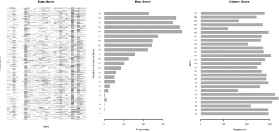
3.5 Geometrical representation of the MCP penalty in 3 dimensions. 34 4.1 INVALSI dataset example: visualization of the data. . . 49
4.2 INVALSI dataset example: solution path of the SPC with ω= 0.5on the INVALSI reduced dataset. . . 51
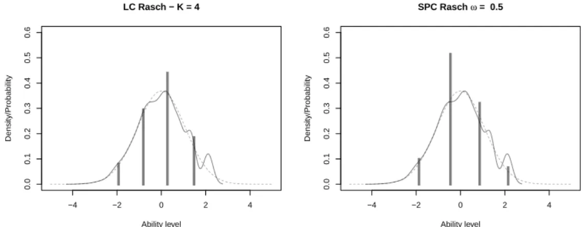
4.3 INVALSI dataset example: estimated distribution of the abil-ity under the Rasch model with the assumption of normalabil-ity (continuous lines) and discreteness (vertical bars) by latent classes (LC) or by sparsication (SPC). . . 51
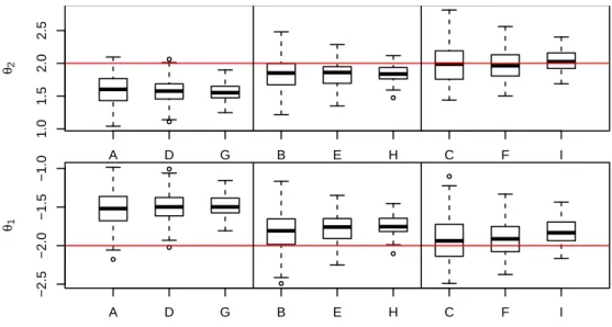
4.4 Simulation study: solutions of the SPC with ω = 0.9for K = 2 (boxplots in 9 scenarios grouped by number of items with increasing sample size). . . 56
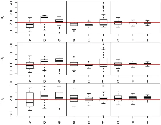
4.5 Simulation study: solutions of the SPC with ω = 0.9for K = 3 (boxplots in 9 scenarios grouped by number of items with increasing sample size). . . 57
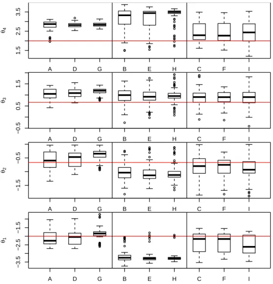
4.6 Simulation study: solutions of the SPC with ω = 0.9for K = 4 (boxplots in 9 scenarios grouped by number of items with increasing sample size). . . 58
5.1 INVALSI scores data. . . 69
5.2 INVALSI scores example: SPC algorithm. . . 70
5.4 Simulation study: solutions of SPC with ω = 0.85for K = 2
(boxplots in 6 scenarios). . . 72 5.5 Simulation study: solutions of SPC with ω = 0.85for K = 3
(boxplots in 6 scenarios). . . 73 5.6 Simulation study: solutions of SPC with ω = 0.85for K = 4
(boxplots in 6 scenarios). . . 74 1 Simulation study: solutions of LC, CL and SPC with ω = 0.9
for K = 2 (boxplots in 9 scenarios). . . 85
2 Simulation study: solutions of LC, CL and SPC with ω = 0.9
for K = 3 (boxplots in 9 scenarios). . . 86
3 Simulation study: solutions of LC, CL and SPC with ω = 0.9
for K = 4 (boxplots in 9 scenarios). . . 87
4 Simulation study: solutions of the SPC with ω = 0.5 in 4
selected scenarios for K = 3. . . 88
5 Simulation study: solutions of the SPC with ω = 0.5 in 4
selected scenarios for K = 4. . . 89
6 Simulation study: SPC estimates of the β parameters in the
scenarios with J = 20. . . 90
7 Simulation study: SPC estimates of the β parameters in the
List of Tables
4.1 INVALSI dataset example: selection of the SPC solutions with the dierence ratio criterion. . . 50 4.2 INVALSI dataset example: estimated ability levels and their
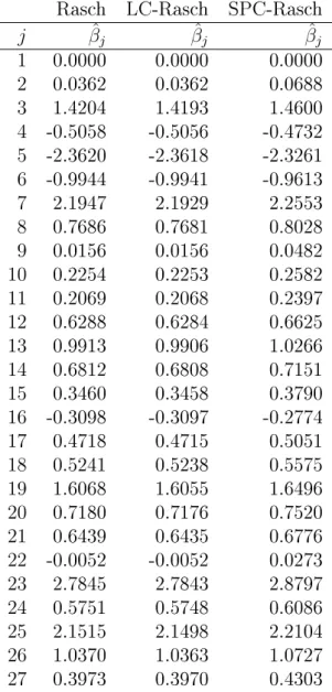
frequencies for the Rasch model, the LC Rasch model and the SPC with ω= 0.5. . . 52
4.3 INVALSI dataset example: estimated diculties for the Rasch model, the LC Rasch model and the SPC with ω= 0.5. . . 53
4.4 Simulation study: scenarios. . . 55 4.5 Simulation study: mean squared error of the estimated
abili-ties of LC, CL and SPC withω = 0.9 in 27 scenarios. . . 59
4.6 Simulation study: mean squared error of the estimated abil-ities for the SPC with ω = 0.5 in 8 selected scenarios with K = 3 and K = 4. . . 61
5.1 INVALSI scores example: SPC estimates for θk, with k = 1, . . . ,4(in brackets the size of each group), empirical meansy¯k of the sucient statistics inK groups dened by a hierarchical
agglomeration (for Complete link and Ward method) forK = 2and K = 4. . . 70
5.2 Simulation study: mean squared error of the estimated abili-ties of SPC withω = 0.85in 6 scenarios with K = 2. . . 75
5.3 Simulation study: mean squared error of the estimated abili-ties of SPC withω = 0.85in 6 scenarios with K = 3. . . 75
5.4 Simulation study: mean squared error of the estimated abili-ties of SPC withω = 0.85in 6 scenarios with K = 4. . . 75
5.5 SPC estimates of theβ parameters (mean values) and relative
mean squared errors in the scenarios withJ = 20. . . 77
1 Simulation study: mean squared error of the estimated abili-ties of LC, CL and SPC withω = 0.9 in 27 scenarios. . . 84
2 Simulation study: mean squared error of the estimated abil-ities for the SPC with ω = 0.5 in 8 selected scenarios with K = 3 and K = 4. . . 89
3 SPC estimates of the β parameters (mean values) and relative
Chapter 1
Introduction
In the era of big data statisticians are faced with the challenging task to develop more and more exible and ecient methods in order to handle the increasing complexity of data structures. We are drowning in information and starving for knowledgeis the motto cited by Hastie et al. (2015) in their inspiring book on statistical learning. Thus, a modern data scientist has the impelling need to dive into this huge mass of information, reducing it to its bare essential. In particular, when building a statistical model, one should al-ways follow the basic principle for which less is more, enhancing parsimony and promoting simplicity over complexity. A problem arises since simplicity is a general, not univocal concept, that may be attained and interpreted in many dierent ways. We refer specically to the following interpretations:
• We interpret simplicity as a result of dimension reduction every time
we try to synthesize high-dimensional data extracting a number of in-formative and non-redundant features. For example, the derivation of these features can be based on a direct projection of the data onto a new space with fewer dimensions, as in Principal Component Analysis (PCA), or it can be the result of a theoretical set of assumptions, as when we deal with a latent variable model (LVM);
• We interpret simplicity as sparsity every time we are interested in
re-ducing the number of non-zero parameters in a model, for example in order to identify a smaller subset of important variables in a re-gression problem. Sparsity can be attained applying a penalization in the estimation process, and many regularization techniques have been developed to produce the so-called shrinkage eect.
The idea beyond this work is to enhance the rst form of simplicity using the properties of the second one. In other words, we propose to overcome some limitations of latent variable modeling, in those cases when the number of parameters directly grows with the dimension of the data, by the means of a well designed sparsication strategy.
In latent variable models we assume that many observed variables are realizations of fewer unobservable ones, synthesizing a certain proportion of the available information (Bartholomew et al., 2011). Latent variables can be dened as variables which are not susceptible of direct measurement, but that in some way aect a set of observed responses. Apart from dimension reduction, there are many reasons for which we may want to include latent variables in a statistical model, typically:
• Represent individual characteristics that cannot be directly measured,
such as intelligence, satisfaction or ability;
• Account for measurement errors, where the latent variables represent
the true outcomes of which the responses represent a disturbed version;
• Represent the eect of unobservable covariates and then accounting for
the so-called unobserved heterogeneity between subjects;
• Account for particular data structures, especially in the presence of
repeated observations, longitudinal/panel data and multilevel data. The idea at the basis of latent variable models is the principle of local independence, for which if a latent variable underlies a series of observed vari-ables, then conditioning on that latent variable makes the observed variables statistically independent. Latent variable models are a wide and heteroge-neous family, and are usually classied according to two criteria (Skrondal & Rabe-Hesketh, 2007): the nature of the response variables and the nature of the latent variables, which could be in both cases discrete or continuous. Here we list some of the most important examples of latent variable models:
• Factor analysis (Child, 2006), a classical tool in multivariate statistics,
which summarizes several continuous measurements through a small number of continuous latent traits, called factors;
• Generalized linear mixed models (GLMMs) (McCulloch & Neuhaus,
2001), also referred to as random-eects models, that represent an ex-tension of the class of generalized linear models (GLM) for continuous or categorical responses which account for unobserved heterogeneity, beyond the eect of observable covariates;
• Item Response Theory (IRT) models (Hambleton & Swaminathan,
1985; Bartolucci et al., 2015), commonly used in questionnaire anal-ysis and Psychometrics. In IRT we typically model categorical items measuring a common latent trait, assumed to be continuous, or less often discrete, representing an ability or a psychological attitude;
• Latent class analyses (Lazarsfeld et al., 1968), that models a set of
categorical response variables with a discrete latent variable, the levels of which correspond to latent classes in the population;
• Finite mixture models (Lindsay, 1995; McLachlan & Peel, 2004), in
which subjects are assumed to come from dierent subpopulations cor-responding to dierent levels of a discrete latent variable, each pop-ulation or cluster being characterized by a dierent distribution of the response variables. The conditional distribution of the responses and/or the distribution of the latent variable can also be aected by observable covariates in nite mixture regression models (Skrondal & Rabe-Hesketh, 2004);
• Latent Markov models (LMM) (Zucchini & MacDonald, 2009;
Bar-tolucci et al., 2012) for longitudinal data, in which the response vari-ables are assumed to depend on a Markov process with unobservable discrete states.
Beyond the nature of the involved variables, another important distinc-tion between latent variable models concerns the estimadistinc-tion process. We can distinguish two alternative approaches, based on dierent sets of assump-tions on the latent structure of the underlying model, and facing dierent computational challenges:
• The random-eects approach, where we consider the latent variables
as random variables attaining a specic value for each sample unit;
• The xed-eects approach, where we treat the values attained by the
latent variables for each sample unit as xed parameters.
The random-eects approach is widely used, because of the lower num-ber of parameters to be estimated, and the high exibility in modeling data structures. It however has several drawbacks, since it involves an a priori assumption on the distribution of the latent variable, that could be miss-specied. Under the xed-eects approach we avoid such assumption but, on the other hand, we end up with a number of parameters to be estimated that is proportional to the size of the data. In this case latent variables are interpreted as sets of individual-specic parameters, and if we are modeling time variant constructs as in LMM then they generate both individual- and time-specic parameters. Namely, if we specify a latent variable model for longitudinal data, an increase in the sample size or in the number of time points will correspond to an increase in the complexity of the model itself. We propose to act in the opposite direction, following the example by Tutz
& Oelker (2017), to promote simplicity by the means of a well suited penal-ization, inducing sparsity.
But what do we mean with sparsity? Generally speaking, we can say that sparsity is high in a model where only a small number of parameters plays an important role (Hastie et al., 2015). We we call such a model sparse. For example, we can say that a linear regression model is sparse when only a limited subgroup of the predictors is considered to be meaningful and is asso-ciated with non-zero coecients. This is the reason why a sparsity inducing process, that allows features selection, can be seen as a classical statistical learning tool (James et al., 2013). This learning task in the framework of the least squares estimation of linear models can be performed with the use of alternative methods, both classical and modern:
• We can perform a classic subset selection. In a model withJ predictors
we can use inferential tools and stepwise methods to identify a subset of sizeJ0 of the predictors, withJ >> J0, which we believe are
signif-icantly related to the response, and then t the model on the reduced set of theJ0 selected covariates;
• We can perform dimension reduction before tting the model, for
ex-ample by the means of Principal Component Analysis or Factor Anal-ysis. In other words we can project a J-dimensional problem into an J0-dimensional subspace, and then t the model;
• We can use a regularization technique introducing a shrinkage operator,
which consists in adding a penalty term when solving the least squares optimization problem. In this case the model is tted with all the
J predictors, but the estimated coecients are shrunk towards zero.
Depending on the type of penalty some coecients may be shrunk exactly to zero, performing this way an automatic variable selection. By retaining a subset of the predictors and discarding the rest, subset selection produces a model that is more interpretable and that has possibly lower prediction error than the full model. However, because it is a discrete process, since at each step variables are either retained or discarded, it often exhibits high variance. Shrinkage methods are more continuous, and do not suer as much from high variability (Friedman et al., 2001).
The two best-known regularization techniques for a regression problem are ridge regression (Hoerl & Kennard, 1970) and the lasso (Tibshirani, 1996):
• Ridge regression is particularly useful when there are many correlated
variables in a linear regression model. It shrinks the regression coe-cients toward zero by imposing a penalty on their size, which alleviates the eects of multicollinearity. The ridge coecients minimize the ob-jective function penalized by the sum of squares of the parameters. Since the shrunk parameters simultaneously reach zero, ridge regres-sion does not perform an automatic feature selection;
• The lasso in a regression problem allows a continuous subset selection,
and it consists in penalizing the objective function by the sum of the absolute value of the parameters. Forcing the sum of the absolute value of the regression coecients to be less than a xed value, it induces certain coecients to be set exactly to zero, eectively choosing a simpler model that does not include those coecients.
The lasso has known a huge popularity and it has been generalized to t many dierent needs. For example, with a well suited penalty we can force some parameters to be shrunk to a given value, rather than zero, or to be sim-ilar among each other, penalizing the objective function on their dierences. Some of the most interesting extensions of the lasso are:
• The elastic net, which combines and generalizes ridge and lasso
regu-larization introducing a tuning parameter that controls the prevalence of one type of shrinkage on the other;
• The group lasso, which allows for a grouped shrinkage of the
param-eters, so that the coecients in the same group are shrunk to zero in the same moment;
• The fused lasso, which penalizes the objective function by the absolute
value of the dierences of consecutive coecients, so that the coe-cients are forced to vary in a smooth fashion, for example in order to respect a certain spatial or temporal structure.
Fused-type penalties have also been used to perform unsupervised clas-sication of statistical units, inducing sparsity on the pairwise dierences of group centroids. Many dierent specications of the pairwise fused lasso penalty have been proposed under dierent names in relatively recent lit-erature. We will use the term convex clustering to refer in general to this whole family of clustering methods exploiting shrinkage techniques to per-form grouping.
Our proposal is to apply a peculiar pairwise fused lasso penalty in the framework of the xed-eects estimation of latent variable models in order to induce a natural clustering on a subset of the parameters space. The idea of clustering xed eects has been widely explored in the work of Tutz, we refer in particular to Tutz & Oelker (2017), where the unobserved heterogeneity is treated using the grouping property of pairwise fused lasso regularization, and Berger & Tutz (2018), where the xed eects are grouped using a recur-sive partitioning method.
In the present work we face this issue by adapting the Solution Path Clustering (SPC) algorithm, which was originally proposed in Marchetti et al. (2014) as a general unsupervised clustering method, to the estimation of grouped xed eects. We believe the SPC to be particularly suited for our purpose for the following reasons. It applies a very exible non-convex penalty on the pairwise dierences of the parameters, promoting sparser models than the `1 penalty with the same or superior accuracy. It does
not require previous knowledge on the number of groups, and it produces a complete solution path, regulated by a single tuning parameter. The tuning process is data-driven, and it can be adapted to datasets of dierent complex-ity. Furthermore, the SPC has the important property of naturally isolating singletons or very small clusters of outliers, that could bring severe bias if included in the estimation of group parameters.
We are the rst to propose the SPC as an estimation tool in the xed-eects latent variable models framework. We think that this method can lead to very good results in terms of accuracy of the estimates, particularly in models with a very large number of free parameters. The aim of this the-sis is to develop a general estimation procedure based on the SPC, and to evaluate its performance, also compared to other methods, in latent variable models characterized by a growing amount of complexity. We are interested in exploring the case of both categorical and continuous data, evaluating the accuracy of the SPC estimates under dierent scenarios, with growing sam-ple size and number of item variables. We choose to focus rst on the most popular IRT model for binary data, the Rasch model (Fischer & Molenaar, 2012), and then on a linear latent variable model for continuous items, where the number of xed eects to be estimated is higher.
The work is structured as follows:
• In Chapter 2 we discuss the xed-eects estimation of latent variable
models. We present the theoretical framework under the xed-eects approach of the classic Rasch model for binary data;
• In Chapter 3 we illustrate the lasso technique applied to linear
regres-sion, and we present the main generalizations of the lasso penalty. We then discuss convex clustering, with particular attention to the algo-rithm by Marchetti et al. (2014);
• In Chapter 4 we present the proposed estimation method for the
pe-nalized xed-eects Rasch model. We introduce the classication like-lihood as an alternative approach to group xed eects in this context. We perform a simulation study to compare the performance of the proposed method with the latent class approach and the classication likelihood. We show the results of a real data example on INVALSI data.
• In Chapter 5 we present the proposed estimation method for the
penal-ized xed-eects latent variable model for continuous data. We perform a simulation study and develop a real data example on INVALSI scores. The concluding remarks are dedicated to the future development of the work, in particular to the extension of the proposed estimation method to the penalized xed-eects variable-intercept model for longitudinal data.
Chapter 2
Fixed-Eects Latent Variable Models
2.1 Latent Variables as Fixed or Random Eects
Latent variables are theoretical constructs which cannot be directly ob-served, but whose values can be inferred on the basis of several other manifest variables (Bartholomew et al., 2011). The use of latent variables is extremely popular in many elds of human knowledge, from Economics to Biology, from Medicine to Sociology, but they are historically relevant in particular to the eld of Psychology (Borsboom et al., 2003). The conceptual framework of latent variable analysis originates indeed in the context of intelligence testing with the work of Spearman (1904). For instance, it is not possible to directly measure the mathematical ability of a student, but we can easily measure his or her performance at a number of test items in mathematics. The observed answers to the items of this questionnaire are then assumed to be proxies of the latent ability (Crocker & Algina, 1986; Raykov & Marcoulides, 2011). Hence, the latent variable is indirectly measured through a statistical model. In this chapter we focus on Item Response Theory (IRT) models (Hamble-ton & Swaminathan, 2013; van der Linden & Hamble(Hamble-ton, 2013), where the probability to provide a certain answer to a questionnaire item is dened as a function of a set of parameters characterizing the items, and of a person's level on the latent trait.
The conceptual status of this unobservable entity is tightly connected to the mathematical formulation of the statistical model. So, the distinc-tion between the xed-eects approach and the random-eects approach in latent variable models contributes not only to determine their parametriza-tion, since it primarily concerns the nature itself of the latent constructs. In the random-eects approach, the individual levels of the latent trait are considered to be realizations of a random variable, characterized by a certain distribution in the population from which the sample has been drawn. This distribution has to be postulated, and it can be either continuous, usually normal, or discrete, allowing for the identication of latent classes in the
population. On the other hand, under the xed-eects approach, the indi-vidual levels of the latent trait are included in the model as unknown xed subject-specic parameters.
A wide literature is dedicated to a comparison between the two ap-proaches, mainly in the framework of generalized linear mixed models (Skro-ndal & Rabe-Hesketh, 2004), and in particular on multilevel models for hi-erarchical, grouped or longitudinal data (Gardiner et al., 2009; Clarke et al., 2010; Townsend et al., 2013). Regardless of a specic model, the choice between xed and random eects depends on a number of theoretical and practical considerations listed in the following:
• Ontology, we have to clarify the nature of the latent construct.
Un-der the xed-eects approach the latent variable is consiUn-dered as an intrinsic attribute of the individual, while under the random-eects ap-proach it is an attribute of the population, characterized by a known distribution. The exibility in dening this distribution allows us to handle a high level of complexity (multidimensionality, hierarchies, group structures, time dependencies) that under the xed eect ap-proach would be problematic.
• Parsimony, the number of parameters to be estimated increases
dra-matically under the xed-eects approach. In particular, apart from the structural parameters of the chosen latent variable model, we also have to estimate at least one parameter measuring the latent trait for each individual in the sample. On the other hand, the random-eects approach requires us to only estimate the parameters of the postulated distribution, together with the structural parameters.
• Assumptions, the subjectivity in dening the latent variable
distri-bution under the random-eects approach may lead to misspecication and related problems. Many works inquiry about the impact of mis-specication of the random eect distribution on the estimators e-ciency (Heagerty & Kurland, 2001; Agresti et al., 2004; Litière et al., 2008; McCulloch & Neuhaus, 2011). A wide literature faces this issue avoiding any distributional assumption through non-parametric estima-tion methods, as for example the recent work of Kelava et al. (2017), or going back to Aitkin (1995) and Laird (1978).
Following from the above example about a questionnaire in mathematics, if we are interested in estimating the latent ability of the respondents, we should consider initially whether or not it is reasonable to formulate a distributional assumption about it, and then choose which one ts best our data. Is the
ability normally distributed? Or is its distribution discrete? Can we isolate groups of respondents with homogeneous ability level?
In order to answer to these questions, in the present chapter we focus on a particular class of IRT model: the binary Rasch model (Rasch, 1960, 1961) or 1PL model, according to the nomenclature in Birnbaum (1968). We illustrate its basic formulation, and we discuss further details about its interpretation and estimation respectively under the xed-eects and the random-eects approach. The Rasch Model is the most widespread among the IRT models for binary data, and we have chosen to use it as a baseline to emphasize the limitations of the xed-eects approach in latent variable models for cross-sectional data.
2.2 The Rasch Model
2.2.1 NotationWe observe the responses of n subjects to J binary items, and we denote
with yij the response of subject i to item j, where i = 1, . . . , n and j =
1, . . . , J. We indicate with yij = 1 the correct answer of responded ito item
j (where yij is the realization of the random variable Yij). We also denote byyi = (yi1, . . . , yiJ)
0
the response pattern of subject i, and withY the data matrix of size n×J, with columns yj = (y1j, . . . , ynj)
0 : Y = y11 y12 · · · y1J y21 y22 · · · y2J ... ... ... ... yn1 yn2 · · · ynJ . (2.1)
We can now dene some quantities of interests such as the total score yi·
of respondent i (row score) and the total scorey·j for itemj (column score)
yi·= J X j=1 yij and y·j = n X i=1 yij (2.2)
which correspond respectively to the number of items endorsed by subject i
and the number of subjects who endorsed itemj. These descriptive statistics
represent a rst raw approximation of the individual's ability and easiness of the item (Baker, 2001).
2.2.2 The model
The Rasch model is the most popular IRT model for binary data. It was introduced by Rasch (1960), and it is based on an item characteristic curve
(ICC) of logistic type. The ICC denes the conditional probability pj(θi)of a correct response of individual i to item j as a function of the individual
latent trait level, indicated with θi. We can write:
pj(θi) = p(Yij = 1|θi) =
eθi−βj
1 +eθi−βj =logit
−1
(θi −βj), (2.3) where βj is a parameter which describes the diculty of item j. Bothθi andβj are dened inRand they are measured on the same scale, allowing for a direct comparison. The item dicultyβj can be interpreted as the level of ability for which subjectihas a probability equal to 0.5 of giving the correct
answer to itemj, given his ability level θi. In particular we havepj(θi) = 0.5 when θi = βj, pj(θi) > 0.5 when θi > βj, and pj(θi) < 0.5 when θi < βj. In this way an item characterized by a high diculty will require a higher value of the latent ability in order to be endorsed. We can consider the item diculty as a location parameter, since it identies the point on the latent continuum at which the latent trait of a subject is located.
Equation (2.3) incorporates three fundamental assumptions (Crocker & Algina, 1986) that must be respected by all IRT models for binary data that are:
• Unidimensionality, which states that the responses to theJitems by
every individuali depend solely on a singular latent trait level θi ∈R, and no other variables are involved in the response process.
• Monotonicity, according to which the ICC is a monotonic
non-decresing function of θi. This is true for the logistic link function,
that has an increasing S-shape, which approaches 0 for θi → −∞ and 1 for θi → +∞. This assumption guarantees that the proba-bility of endorsing an item increases with an increase of the aproba-bility level of the respondent. Conversely the probability of success decreases as the diculty parameters βj increases. Figure 2.1 represents the ICC as a function of θi for ve items having dierent diculty levels
β1 < β2 < β3 < β4 < β5.
• Local independence, which states that the responses to theJ items
for each subjectiare conditionally independent given the latent ability
level θi. In other words, if the true levels of ability were known, the
response of individual i to an item j would not give any additional
information in predicting the response of the same individual to any other item. In the same way an individual with an higher ability level will respond better to any item with respect to an individual on a lower
Figure 2.1: Item characteristic curves of a Rasch model for 5 items with increasing diculty levels.
position on the latent trait. Thanks to this assumption we can write the joint distribution of a response pattern yi given θi as follows:
p(yi|θi) = J Y j=1 pj(θi)yij[1−pj(θi)] 1−yij . (2.4)
Plugging in Equation (2.3) in (2.4) we obtain the explicit expression of the conditional probability for the Rasch model
p(yi|θi) = J Y j=1 eyij(θi−βj) 1 +eθi−βj = eyi.θi−PJj=1yijβj Qp j=1(1 +eθi −βj). (2.5)
Recalling the implicit assumption that the response vectors corresponding to dierent subjects in the sample are independent to each other, we can write the conditional probability of observing the response matrix Y given the ability vectorθ = (θ1, . . . , θn)
0 , as: p(Y|θ) = n Y i=1 p(yi|θi) = n Y i=1 eyi.θi−Ppj=1yijβj QJ j=1(1 +eθi−βj) = e Pn i=1yi·θi− PJ j=1y·jβj Qn i=1 QJ j=1(1 +eθi−βj) (2.6) .
2.2.3 Fixed Eects or Random Eects
As mentioned in Section (2.1), under the random-eects approach the level θi of the latent ability in a Rasch model is considered as a realization of a random variable Θi with density function f(θi). Consequently, starting by Equation (2.4), we can obtain the marginal distribution of the response patternyi by integrating out the latent trait
p(yi) =
Z
R
p(Y|θ)f(θi)dθi (2.7) where the density function f(θi) is common to every subject. The quantity
p(yi) is also known as manifest distribution (Bartolucci et al., 2015). The random-eects approach has to be adopted when the group of respondents is considered a sample drawn from a population, the ability of which we know is characterized by a certain continuous or discrete distribution.
On the other hand, under the xed-eects approach the ability levels
θ1, . . . , θnare considered as subject-specic parameters to be estimated along with the diculty parameters. We can interpret the row scores(y1·, . . . , yn·)
0
as a set of minimal sucient statistics forθ, since the distribution with
prob-ability expressed by Equation (2.6) belongs to the exponential family, whose canonical parameters are a linear function of θ and β. The suciency ofyi·
implies that individuals sharing the same number of endorsed items will also obtain the same estimate of the ability, independently from possible dier-ences in their specic response patterns. In a similar way, the column scores
(y·1, . . . , y·J)
0
represent a minimal sucient statistic for the parameter vector
β. Adopting the xed-eects approach we are not making any assumption
concerning the population, we refer to a xed group of subjects, each carry-ing an intrinsic value of the parameter, and we assume that the variability between repeated responses of the same subject to the same item is due only to accidental factors.
The choice between xed-eects and random-eects implies dierent es-timation strategies, each one characterized by its own advantages and disad-vantages (Bartolucci et al., 2015). We distinguish:
• joint maximum likelihood (JML) under the xed-eects approach,
it consists in maximizing the likelihood of the model with respect to the abilities and the diculties jointly. This is the method we will use to estimate the latent ability, and it will be extensively described in the next paragraph.
• conditional maximum likelihood (CML) under the xed-eects
function of only one set of parameters, either abilities θi or diculties
βj. The conditional likelihood, given the sucient statistics for one set
of parameters, is maximized with respect to the other using a Newton-Raphson algorithm.
• marginal maximum likelihood (MML) under the random-eects
approach, it consists in maximizing the likelihood of the model after the ability parameters have been integrated out on the basis of a common known distribution. The ability is usually assumed to be Gaussian with arbitrary parameters µ and σ2. The maximization is performed using
the expectation maximization (EM) algorithm (Dempster et al., 1977). 2.2.4 Estimation with the Joint Maximum Likelihood
The JML method involves the maximization of the Rasch model likelihood with respect to both ability and diculty parameters simultaneously. For this reason we aggregate all the xed-eects parameters in a single vector
ψ = (θ,β)0, and directly use Equation (2.6) to dene the model likelihood
function as: L(ψ) = e Pn i=1yi·θi−PJj=1y·jβj Qn i=1 QJ j=1(1 +eθi−βj) , (2.8)
with corresponding log-likelihood:
`(ψ) = logL(ψ) = n X i=1 yi·θi− J X j=1 y·jβj − n X i=1 J X j=1 log 1 +eθi−βj. (2.9)
The above quantity can be expressed in vector notation
`(ψ) =y0rθ−y0cβ−10nlog1 +eθ10J−1nβ0
1J, (2.10)
where yr = (y1·, . . . , yn·)0 and yc= (y·1, . . . , y·J)
0
are respectively the vectors of the row and column scores (containing the sucient statistics for the model parameters), the symbol 1h indicates a vector of ones of generic length h,
and log(1 +eθ10J−1nβ0) is a n ×J matrix of elements log(1 +eθi−βj), with
i= 1, . . . , n and j = 1, . . . , J. log(1+eθ10J−1nβ0) =
log(1 +eθ1−β1) log(1 +eθ1−β2) · · · log(1 +eθ1−βJ)
log(1 +eθ2−β1) log(1 +eθ2−β2) · · · log(1 +eθ2−βJ)
... ... ... ...
log(1 +eθn−β1) log(1 +eθn−β2) · · · log(1 +eθn−βJ)
. (2.11)
A problem arises since both L(ψ)and `(ψ) are invariant with respect to
translations of the parameters θi and βj. The reason is that if in Equation (2.3) we add a constant to every ability parameter and every diculty pa-rameter, such that θi∗ =θi +cand βj∗ =βj +c, then p∗j(θi∗) = pj(θi). This makes the model non-identiable, and in order to reach an estimate ofψ we
have to put suitable identiability constraints on some parameters. One may choose between:
• Setting to zero the rst item diculty β1 = 0. In this case the rst
item is taken as a reference item, in the sense that we interpret the other diculty parametersβj wherej = 2, . . . , J with respect to it.
• Setting to zero the average diculty level PJ
j=1βj = 0 or the average
ability level Pn
i=1θj = 0, so that the parameters estimates are inter-preted as deviations from the mean.
The two constraints are equivalent, leading to a maximum likelihood value equal to the unconstrained maximum likelihood. Besides, the estimates ob-tained under one identication rule can be easily transformed into the es-timates obtain under the other one. In this work we choose to adopt the rst one, resulting the new vector of free parameters as ψ = (θ,β∗)0, where
β∗ = (β2, . . . , βJ)
0
.
The log-likelihood (2.9) can be maximized using a Newton-Raphson it-erative algorithm that at each step updates the parameter estimates until convergence (Bartolucci et al., 2015). In more detail, leth= 1, . . . , H be the
iteration index, and ψ(h) be the ψ estimate obtained at steph, abilities and
diculties are updated as follows
θ(ih+1) =θi(h)−∂`(ψ (h)) ∂θi " ∂2`(ψ(h)) ∂θ2 i #−1 and βj(h+1) =βj(h)−∂`(ψ (h)) ∂βj " ∂2`(ψ(h)) ∂β2 j #−1 (2.12) where i = 1, . . . , n and j = 2, . . . , J, the rst and second derivatives with
respect toθi are: ∂`(ψ(h)) ∂θi =yi·− J X j=1 pj(θi) and ∂2`ψ(h) ∂θ2 i =− J X j=1 pj(θi) [1−pj(θi)], (2.13)
and the rst and second derivatives with respect to βj are: ∂`(ψ(h)) ∂βj =− " y·j − n X i=1 pj(θi) # and ∂ 2`ψ(h) ∂θ2 i =− n X i=1 pj(θi) [1−pj(θi)], (2.14) where pj(θi) is dened as in Equation (2.3). Starting from expression (2.10), we can write the gradient ∇ψ and the HessianHψ in vector notation:
∇ψ = yr−P1J −yc+P01n , (2.15) Hψ = diag{[P(1−P)]1J} [P(1−P)] [P(1−P)]0 diag[P(1−P)]01n , (2.16)
where Pis a n×J matrix of elements
P= p1(θ1) p2(θ1) · · · pJ(θ1) p1(θ2) p2(θ2) · · · pJ(θ2) ... ... ... ... p1(θn) · · · pJ(θn) . (2.17)
and [P(1−P)] is a matrix of the element-wise products pj(θi) [1−pj(θi)]. The algorithm can be initialized with arbitrary values ψ(0). The choice
for the initialization is not extremely relevant being `(ψ) a strictly concave
function in the parameter space. Bartolucci et al. (2015) suggest to use a data driven initialization
θ(0)i = log yi· J −yi· and βj(0) = logn−y·j y·j −logn−y·1 y·1 (2.18) for i= 1, . . . , n and j = 2, . . . , J.
If properly initialized the algorithm converges reasonably fast to the JML estimate ψˆ= (θˆ,βˆ)0. A convergence rule based on both the maximum
like-lihood dierence at consecutive steps and the distance between consecutive solutions can be adopted.
`(ψ(h))−`(ψ(h+1))< ε1 and max|ψ(h)−ψ(h+1)|< ε2 (2.19)
with ε1 and ε2 small constants.
However, the JML estimate is not guaranteed to exist, Fischer (1981) provides a set of conditions on the matrix Y that ensures the existence of
the JML estimate. A necessary condition is that in that 0 < yi· < J for
i = 1, . . . , n and 0 < y·j < n for j = 1, . . . , J, namely that there are no subjects that responded correctly or incorrectly to all items and that there are no items to which all subjects responded correctly or incorrectly. If there are rows and columns with all elements equal to zero or one they have to be eliminated from the dataset.
2.2.5 Latent Class Rasch Model
One unique property of the random-eects approach is the possibility to specify a discrete distribution for the latent construct. In this way, just as in latent class models (Lazarsfeld et al., 1968; Goodman, 1974), we assume that the population under study is composed by a number of classes or sub-populations that are homogeneous in terms of the unobservable construct. A discreteness assumption is particularly convenient when we want to cluster individuals on the basis of their latent ability, or in those cases when we have many items and many dierent values of the sucient statistics yi·. The
la-tent class Rasch (LC-Rasch) model has been proposed by Rost (1990), other examples of this formulation and its extensions can be found in Lindsay et al. (1991), Formann (1995) and Bartolucci (2007).
In general, we assume that the random variable Θi, where i = 1, . . . , n, has a discrete distribution with support pointsξ1, . . . , ξK. Each support point
measures the latent ability of the k-th latent class, with associated support
points πk, k = 1, . . . , K, representing the probability that a subject belongs
to classk, given by
πk =p(Θi =ξk), (2.20)
with PK
k=1πk and πk ≥ 0, k = 1, . . . , K. Assuming that the diculty pa-rameters are constant across classes, we can write the ICC as:
pj(ξk) = p(Yij = 1|ξk) =
eξk−βj
1 +eξk−βj. (2.21)
As in the case of continuous latent variable, the estimation of the parameters is based on the MML method and solved by the EM algorithm. Alternatively, in Lindsay et al. (1991) the LC Rasch model is interpreted and estimated as a nite mixture model.
2.2.6 Limits of the JML
We have seen how the JML estimation of the Rasch model under the xed-eects approach is simple and straightforward, but it has several relevant drawbacks with respect to the MML estimation under the random-eects approach:
• The main drawback is the lack of consistency of the resulting estimator
forJ xed asn grows to innity. The reason is that the number of the
ability parameters increases with the sample size.
• The number of dierent values of the ability parameters estimates is
equal to the number of dierent values of the sucient statistics yi·.
This may represent a drawback when we desire a group structure like in LC Rasch Model, and in all those cases when we desire a number of unique values for the estimates θˆ that is lower than the number of
unique values of the sucient statistics in yr.
Chapter 3
An Overview on Lasso-Type Penalties
3.1 The Lasso
The lasso (least absolute shrinkage and selection operator) was rst in-troduced by Tibshirani (1996) as a method for both shrinkage and selection in a general regression framework. It is a continuous shrinking operator, it allows automatic variable selection, and it always leads to sparse solutions. This properties gained the lasso a huge popularity, and it has become quickly a fundamental tool in statistical learning (Friedman et al., 2001; James et al., 2013; Hastie et al., 2015). Other standard techniques, such as ridge regression (Hoerl & Kennard, 1970) and subset selection algorithms, had the drawback to perform either only shrinkage or variable selection. In particular, stepwise methods, like forward selection and backward elimination, are likely to pro-duce unstable outputs, being discrete processes based on a certain selection criterion. On the other side, the lasso is based on the penalization of a loss function by the `1-norm of the parameter vector. It results in a quadratic
programming problem with linear inequality constraints. In practice, it forces a subset of regression coecients to be exactly equal to zero, imposing the sum of their absolute values to be less or equal than a user-specied tuning parameter.
3.1.1 Notation
In the framework of generalized linear models (GLM) (Nelder & Baker, 1972; McCullagh, 1984) we observe n values of the response variable Y,
which can be either continuous or binary, and of a set of predictorsXj, with j = 1, . . . , J. We can denexi = (x1i, . . . , xJ i)as theJ-dimensional vector of predictors, and each yi ∈Ras the associated value of the response variable. The vectorsxi are stacked as rows of the n×J matrix of predictors X. The model is parametrized by a vector of regression coecients β= (β1, . . . , βJ)
0
In this chapter we make extensive use of dierent norms that, for the sake of clarity, we explicitly dene here:
• The`1norm, Taxicab norm or Manhattan norm of a vectorβis dened
as the sum of the absolute values of its elements, and it is indicated with the symbols k · k ork · k1:
kβk=
J
X
j=1
|βj|. (3.1)
• The `2 norm or Euclidean norm of a vector β is dened as the square
root of sum of its squared elements, and it is indicated with the symbol
k · k2: kβk2 = p β0β= v u u t J X j=1 β2 j. (3.2)
• The`q norm orq-norm is a generalized norm that is equal to the `1 for
q= 1 and to the `2 for q = 2. It is indicated with the symbol k · kq:
kβkq = J X j=1 |βj|q !1q . (3.3)
3.1.2 The Lasso for Linear Regression
Lets consider a linear regression model of the form:
E(Yi|X) = f(xi) =β0+
J
X
j=1
xijβj, (3.4)
for which the classic ordinary least square estimate( ˆβ0OLS,βˆOLS) is obtained
minimizing the residual sum of squares. The lasso nds the solution βˆ = ( ˆβ0,βˆ) to the constrained optimization problem:
min β0β 1 2 n X i=1 yi−β0− J X j=1 xijβj !2 subject to J X j=1 |βj| ≤t, (3.5)
which can be written more compactly just in vector notation:
min β0β 1 2ky−β01n−Xβk 2 2 subject to kβk1 ≤t, (3.6)
where y = (y1, . . . , yn) is the vector of continuous responses. The tuning parameter t is a predetermined xed scalar, and it can be seen as a sort of
budget, limiting the sum of the absolute values of the parameters estimates, and controlling the desired amount of shrinkage. The value of t is usually
chosen by cross-validation, as will be discussed in Section 3.1.4. The matrix of predictorsX is standardized so that each column is centered and has unit variance, in order to avoid biases due to dierent scales. If we consider the response variable to be centered too, we can omit the intercept term β0 and
rewrite the problem as:
min β 1 2ky−Xβk 2 2 subject to kβk1 ≤t. (3.7)
The optimization problem (3.7) can be expressed also in the Lagrangian form min β 1 2ky−Xβk 2 2+λkβk1 with λ≥0, (3.8)
where, given the strict convexity of both the loss function and the penalty term, by the Lagrangian duality, there is a one-to-one correspondence be-tween λ and t (Bertsekas, 1999). As already mentioned, the structure of
the `1 penalty allows not only the shrinkage of the parameters, but also the
automatic selection of the variables: as the value of t decreases an
increas-ing number of parameters are forced to be exactly equal to zero. Thanks to this property the lasso always leads to sparse solutions, and it becomes more useful when working with large problems, particularly in the case of wide data, when J n. In order to better understand the mechanism beyond
the sparsity-generating process of the lasso penalty, it is useful to look at its geometrical implications, comparing its structure with another common shrinkage technique: the ridge regression. In ridge regression we optimize:
min β 1 2ky−Xβk 2 2 subject to J X j=1 βj2 ≤t2, (3.9)
so that, for decreasing values of t, the parameters are shrunk together, and
they reach 0 only when t = 0. Figure 3.1 shows the proles of the solution
path for the lasso and ridge penalties applied to the estimation of the same linear regression model. We can see how the lasso solutions gradually hit the zero as t decreases, meaning that the corresponding variables can be deleted
from the model, while the ridge regression solutions are shrunk together way more smoothly until they reach zero simultaneously, not allowing for variable selection. Figure 3.2 directly compares the shape of the two constraints in a
Figure 3.1: Solution paths for the lasso (left) and ridge regression (right).
linear regression model withJ = 2. The residual sum of squares has elliptical
contours, and it is centered at the full least-squares estimates. Geometrically speaking, both methods nd the penalized solution where the elliptical con-tours rst hit the constraint region. This area is a diamond|β1|+|β2| ≤t for
the lasso, and a disk β2
1 +β22 ≤ t2 for the ridge regression. Unlike the disk,
the diamond has corners, and if the elliptical contours hits the diamond right on one of its corners, then one parameter βj results exactly equal to zero. WhenJ >2 the diamond becomes a rhomboid, and has many more corners,
increasing the number of opportunities for the estimated parameters to be zero, while the disk becomes a sphere.
Both lasso and ridge regression can be seen as special cases of a general optimization problem subject to an `q penalty, which takes the following Lagrangian form: min β ( 1 2ky−Xβk 2 2−λ J X j=1 |βj|q ) . (3.10)
This problem reduces to the lasso forq= 1 and to ridge regression forq= 2.
For q = 0 the penalty term just counts the non-zero elements of the vector
β, after performing a best-subset selection. Figure 3.3 shows the shape of
the constraint regions corresponding to these penalties for the case of two predictors (J = 2). For values of q greater or equal to one we stay in the
Figure 3.2: Geometrical interpretation of the lasso (left) and ridge regression (right) with J = 2.
Figure 3.3: Constraint regions for a penalty of the general form PJ
j=1|βj|
q with dierent values ofq.
framework of convex optimization, while for q < 1 we have a non-convex
programming problem (which leads to several computational diculties).
Computationally speaking, the lasso problem (3.8) is a convex optimiza-tion program, in particular a quadratic program (QP) with a convex con-straint. As such, many sophisticated QP methods are capable of nding its solutions. However, apart from this general convex optimizers, several al-ternative algorithms have been designed and proposed specically in order to nd the lasso solutions. At rst, in his seminal paper Tibshirani (1996) outlined a combined quadratic programming method, in which the inequal-ity constraints were introduced sequentially, seeking a feasible solution that satised the optimality conditions. A few years later, his student Fu (1998) developed the shooting algorithm, a rst coordinate-wise minimization pro-cedure, derived interpreting the lasso estimator as the right limit of the bridge estimator (Frank & Friedman, 1993) when the order of the penalty norm goes
to one. An ecient alternative is represented by the least angle regression (LAR), proposed by Efron et al. (2004). With respect to earlier methods, LAR had the advantage to produce the entire piecewise linear solution path, instead of returning a single vector solution. This property was particularly appealing in the tuning phase of the model. LAR is sometimes referred to as the homotopy approach, having much in common with an earlier piecewise linear path algorithm for computing the lasso, proposed by Osborne et al. (2000a,b). Finally, working on the idea of Fu (1998), Friedman et al. (2007) developed a coordinate minimization procedure, the cyclical coordinate de-scent, which minimized the convex objective along a coordinate at a time, leading under mild conditions to the global optimum. Iterating the algo-rithm over dierent values of the regularization parameter, it was possible to create the entire solution path, just as for the LAR. The entire algorithm is referred to as pathwise coordinate descent and it is nowadays considered to be the fastest and simplest method to solve the basic lasso problem. For many generalizations of the lasso a correspondent coordinate descent (or as-cent) algorithm has been developed. Also the algorithm that we propose to use in Chapter 4 acts coordinate-wise.
3.1.3 The Lasso for Logistic Regression
The lasso has been widely applied to generalized linear models. Tib-shirani (1996) proposed its application to logistic regression, for which co-ordinate descent algorithm have been later developed by Friedman et al. (2007). In logistic regression we apply the `1 regularization to the negative
log-likelihood: Λ(β) =− 1 N n X i=1 h yi(β0+β0xi)−log 1 +eβ0+β0xi i +λkβk1. (3.11)
The objective is convex and the likelihood part is dierentiable, so nding the solution is a standard task in convex optimization. Coordinate descent type algorithms can be implemented over a quadratic approximation of the likelihood.
3.1.4 Inference and Cross-Validation
The tuning parameter t in the lasso criterion controls the complexity of
the model. It acts like a budget, larger values oft produce more free
param-eters and allow a better t of the model to the data, smaller values induce a stronger shrinkage, reduce the number of non zero parameters, leading to sparser, more interpretable models that t the data less closely. A value of
t that is too small can produce a poorly adapted model, while a large value
can lead to overtting. Cross-validation is the most common strategy to esti-mate the best value fort that strikes a good balance in the trade-o between
goodness of the t and interpretability. In practice, we rst randomly divide the full dataset into some number of groupsK (typically 5 or 10). We choose
one group as the test set, and use the remainingK−1groups as the training
set. We then apply the lasso to the training data over a sequence of dierent
t values, and we use each tted model to predict the responses in the test
set, recording the mean-squared prediction errors for each value of t. After
repeating this K times, so that each group has been used once as test set,
we choose the value of t that minimizes the error measure. With very large
datasets this procedure can be computationally intensive and time demand-ing. More problems arise when the parameters involved in the penalty term are more than one, as it happens in many lasso generalizations.
Concerning inference on the lasso estimates, various standard error es-timators have been proposed. Tibshirani (1996) suggested to compute the standard errors using the bootstrap (Efron, 1979; Efron & Tibshirani, 1986), arguing that a closed form approximation for the covariance matrix leads to a null estimated variance for those predictors with an estimated coecient shrunk exactly to zero. This limitation is shared also by other sandwich for-mulas proposed in Fan & Li (2001) and Zou (2006). Osborne et al. (2000b) derived an approximation formula that yields to a positive error for all the coecient estimates, but pointed out that the estimates may be far from normally distributed. Pötscher & Leeb (2009) showed that the nite sample distribution of the lasso (soft-thresholding) estimator, can be highly non-normal irrespective of sample size, while Knight & Fu (2000) considered its asymptotic behavior. From this ndings, Kyung et al. (2010) proved the inconsistency of bootstrap standard errors if the true coecient is equal to zero. Since the bootstrap can not be considered a general method of ob-taining standard errors of the lasso estimates, Kyung et al. (2010) proposed a fully Bayesian formulation, extending the hierarchical representation sug-gested by Park & Casella (2008). The Bayesian interpretation of the lasso was rst sketched by Tibshirani (1996), and it has been widely applied.
3.2 Generalizations of the Lasso
The good properties of the lasso stimulated much research about pos-sible generalizations of its penalty, to overcome some of its limitations and extend the elds of application. For example, the basic lasso does not
per-form well in the presence of multicollinearity, for this reason Zou & Hastie (2005) proposed the elastic net, that combines the`1-penalty with a squared
`2-penalty, tending to select (or not) the correlated features together.
An-other important generalization is represented by the group lasso, introduced Yuan & Lin (2007), that selects or omits groups of variables, when the groups are known. The group lasso is extremely useful for the correct treatment of polytomous categorical predictors, allowing in variable selection to include or exclude simultaneously all the dummy variables used to code the levels. But lasso-type penalties can be designed to account for many dierent data structures, not only groups. The fused lasso, introduced by Tibshirani et al. (2005), is designed for problems with features that can be ordered in some meaningful way. It encourages local constancy of the coecient prole, pe-nalizing the loss function by the `1-norm of both the coecients and their
successive dierences. The idea of penalizing the dierences of parameters, instead of penalizing the parameters themselves, stimulated much research, and it lead to what is sometimes referred to as convex clustering. This tech-nique and the idea of using a well suited penalty to induce clustering on a set of parameters are at the basis of our proposal, and they will be covered in the last section of this chapter. Before it can be useful to have a closer look to the above mentioned generalizations of the lasso, from which the others in some way descend.
3.2.1 The Elastic Net
The lasso performs poorly when the predictors are highly correlated (Oyeyemi et al., 2015). In case of multicollinearity the solution paths of the lasso tend to be erratic, expressing a wild behavior. The elastic net represents a possible solution to this problem. It consists in a compromise between the ridge re-gression (that was introduced as a way of handling multicollinearity problems in regression) and the lasso penalty. The linear combination that is regulated by a mixing parameter α. The elastic net problem can be expressed as:
min β 1 2ky−Xβk 2 2+λ 1 2(1−α)kβk 2 2+αkβk1 , (3.12)
with λ ≥ 0 and α ∈ [0,1]. Since the penalty associated to an individual
coecient is given by:
(1−α)β2
j +α|βj|
2 , (3.13)
it is clear that when α = 1, the elastic net penalty reduces to the `1-norm,
corresponding to the lasso, while when α = 0 it reduces to the squared `2-norm,corresponding to the ridge penalty. Friedman et al. (2015) built
a system of coordinate-descent algorithms for tting elastic-net penalized generalized linear models.
3.2.2 The Group Lasso
The group lasso encourages sparsity between natural groups of predictors, forcing the βj inside the same group to be shrunk simultaneously to zero. We assume that the design matrix X is composed by G known groups of
predictors, such that X = (X1|X2|. . .|XG), with g = 1, . . . , G. We indicate with Jg the size of the g-th group, corresponding to a set of Jg columns of the matrix X. The group lasso problem can be dened as:
min β ( 1 2ky− G X g=1 Xgβgk 2 2 ) subject to G X g=1 kβgk2 ≤t, (3.14)
where βg is a subvector of β reecting the group structure. The group
generalization of the lasso has two properties:
1. Depending on t (or λ), either the entire vector βg will be zero, or all
its elements will be non zero. In other words sparsity is induced only among groups, not within groups.
2. WhenJg = 1, then we havekβgk2 =|βj|, so if all groups are singletons the group lasso problem reduces to the basic lasso.
In this formulation (3.14) all the groups are equally penalized, but in this way larger groups are more likely to be selected. A possible solution is to weight the penalties for each group according to their size, for example by a factor p
Jg, as suggested by Yuan & Lin (2007).
min β ( 1 2ky− G X g=1 Xgβgk 2 2+λ G X g=1 √ pgkβgk2 ) (3.15)
To solve the problem (3.14) we apply the block coordinate descent, that consists in minimizing the Lagrangian function with respect of thek-th block
of predictors (vector βk), cycling through the G groups while holding xed
all the other block parameter vectors to their current value {βˆj, j 6= k}.
The group lasso has been widely extended. Meier et al. (2009) adapted it to logistic regression problems, while other authores proposed variations of the penalty structure in order to allow for example sparsity within groups or the presence of overlapping groups. These are the cases of the overlap group lasso (Jacob et al., 2009) and the sparse group lasso (Puig et al., 2009; Simon et al., 2013).
• Sparse Group Lasso, For the properties of the `2 norm, when a
group is included into a group-lasso t, all the coecients in that group must be non-zero. Sometimes we may want to induce sparsity not only with respect to which groups are selected, but also with respect to coecients within each group. The sparse group lasso, inspired by the elastic net, is designed to achieve within-group sparsity, augmenting the group-lasso penalty with an additional`1-penalty, through a mixing
parameterα ∈[0,1]: min β ( 1 2ky− G X g=1 Xgβgk 2 2+λ G X g=1 (1−α)kβgk2+αkβgk1 ) , (3.16)
where with α= 0 we get the group lasso and with α= 1 the lasso.
• Overlap Group Lasso, There are cases in which some predictors
may belong to more than one group. The overlap group lasso allows variables to be accounted in all the groups in which they are included. This penalty simply replicates a variable in whatever group it appears, and then ts the ordinary group lasso.
3.2.3 The Fused Lasso
The fused lasso is useful whenever we want to take into account a struc-tural relation between the parameters object of shrinkage. The nature of this relationship can be for example temporal or spatial adjacency. In the linear regression framework a fused lasso problem in its Lagrangian form typically appears as follows: min β 1 2 n X i=1 yi − J X j=1 xijβj !2 +λ1 J X j=1 |βj|+λ2 J X j=2 |βj −βj−1| , (3.17)
where we have two tuning parametersλ1 and λ2, corresponding to two
sepa-rate penalties: the`1 penalty of the base lasso, that shrinks the parameters
towards zero, and the fusion penalty that encourages neighboring coecients
βj to be similar, forcing many of them to be identical. This second penalty makes sense as long as the ordering of the coecients is xed and somewhat informative.
The fused lasso problem cannot be solved using a coordinate descent algorithm, due to the fact that the dierence penalty is not a separable function of the coordinates, but it can be expressed as in Tibshirani et al.
(2011), where the authors propose a solution path algorithm for any lasso problem of the form:
min β 1 2ky−Xβk 2 2+λkDβk1 , (3.18)
whereDis a penalty matrix of sizem×J, beingmthe number of constraints
built on the parameters vector of length J.
In the fused lasso examplem=n−1is the number of dierences between
consecutive elements ofβ, and the matrixDwill have rows in which the non-zero elements are always adjecent couples of −1 and 1:
D = −1 1 0 · · · 0 0 0 −1 1 · · · 0 0 · · · 0 0 0 · · · −1 1 . (3.19)
In Tibshirani et al. (2011) the one-dimensional fused lasso is presented as a simple tool for signal approximation. In their application, since it produces a piecewise constant t, the fused lasso is also used for smoothing purposes:
min θ {Λ(θ)}= minθ ( 1 2 n X i=1 (yi−βi)2+λ1 n X i=1 |θi|+λ2 n X i=2 |θi−θi−1| ) . (3.20) 3.2.4 The Pairwise Fused Lasso
The idea of applying the shrinkage on dierences among parameters in-stead of parameters themselves opened the path for a whole new kind of generalization aimed at reproducing specic parametric structures. In Petry et al. (2011) the authors introduce the pairwise fused lasso (PFL) penalty, that uses the `−1 norm of the pairwise dierences of coecients in a
gen-eralized linear model, extending the fused lasso to the case in which it is not possible to dene a xed ordering of the predictors. The PFL penalty is dened as: Pλ,αP F L(β) = λ " α J X j=1 |βj|+ (1−α) X k<j |βj −βk # , (3.21)
where λ >0 and α ∈[0,1]are the tuning parameters. The rst term in the
is the fusion term and accounts for grouping. Petry et al. (2011) proposes two optimization procedures to solve the problem
min
β
`(β) +Pλ,αP F L(β) (3.22)
where`(β)is the negative loglikelihood of a GLM. One approach is based
on the LARS algorithm from Efron, and the other one on the local quadratic approximation (LQA) of `(β).
The PFL penalty can be expressed as a generalized lasso penalty (Tib-shirani et al., 2011) with matrixDthat selects in each row the j-th andk-th
element of the pairwise dierences, giving respectively value 1and −1. The
D matrix will have J columns and a number of rows m = J2
equal to the number of 2-combinations ofJ elements. For J = 4 we get:
DJ=4 = 1 −1 0 0 1 0 −1 0 1 0 0 −1 0 1 −1 0 0 1 0 −1 0 0 1 −1 and DJ=5 = 1 −1 0 0 0 1 0 −1 0 0 1 0 0 −1 0 1 0 0 0 −1 0 1 −1 0 0 0 1 0 −1 0 0 1 0 0 −1 0 0 1 −1 0 0 0 1 0 −1 0 0 0 1 −1 . (3.23) In other works similar penalties have been proposed, for example She et al. (2010) calls it clustered lasso
3.3 Lasso-Type Penalties for Clustering
The grouping property of the pairwise fusion has been exploited also to perform clustering of the statistical units. In this case, instead of penalizing the coecients of a regression model, the penalty is applied on the dierences among centroids. The shrinkage forces pairs of centroids to converge on the same value, producing an implicit representation of clusters through the occurrence of equal centroids. Given a data matrixY of sizen×p, we assume
each rowyi to be ap-dimensional centroidµi of a singleton. We can express a convex clustering problem as:
min µ ( 1 2kyi−µik 2 2+λ X i<j wijkµi−µjk1 ) (3.24)
where i = 1, . . . , n, j = i, . . . , n, and wij are predetermined weights. Pelck-mans et al. (2005) rst proposed convex clustering as a method to perform clustering by solving a convex optimization problem through a LAR-type al-gorithm. Pan et al. (2013) proposed a penalized regression-based clustering (PRclust), using a non-convex truncated lasso penalty (Shen et al., 2012). We also cite the work of Hocking et al. (2011) and Lindsten et al. (2011). Marchetti et al. (2014) proposed the Solution Path Clustering (SPC), which with a blockwise coordinate approach iterates a Majorization-Minimization (MM) step over a set of data-driven tuning parameters in order to mini-mize an approximation of the objective function under a Minimax Concave Penalty (Zhang et al., 2010). With respect to other techniques, the SPC has the advantage to select automatically the tuning parameters producing a dendrogram-like set of solutions; it does not require the input of the number of clusters, and it is capable of handling and isolating outliers.
3.3.1 The Solution Path Clustering
In Marchetti et al. (2014) the underlying model for each object yi is as-sumed to be a multivariate Gaussian with mean parameter µi ∈ RJ and constant diagonal covariance matrix σ21J. The optimization problem
con-sists in minimizing the criterion function:
ΛK(µ) = K X k=1 X i∈Ck kyi−µkk 2 2+λ X k<l nknlρ(kµk−µlk2), (3.25)
where then observations are organized in K clusters of size nk, with centers µk ∈ RJ and labels Ck, k = 1, . . . , K. The penalty function ρ(·) is the Minimax Convex Penalty (MCP) developed by Zhang et al. (2010):
ρ(t) = t− t 2 2λδ I(t < λδ) + λδ 2 I(t < λδ), with t ≥0, (3.26)
where I(·) is the indicator function. The MCP denes a family of penalties
that are concave int∈[0,∞), whereλ >0controls the amount of
regulariza-tion and δ >0 the degree of concavity. Such non-convex penalties promote
sparser models than the `1 penalty with the same or superior prediction
ac-curacy in regression models. MCP includes both the`1 penalty whenδ ← ∞
and the `0 penalty when δ ← 0+, forming a continuum between the two
extremes.
Figure 3.4 shows the eect of an increase of λ and δ on the shape of the
penalty function ρ(t). In the left panel we keepδ xed to 1 and make λ vary