QATAR UNIVERSITY
COLLEGE OF ARTS AND SCIENCES
INFERENCE ABOUT THE GENERALIZED EXPONENTIAL QUANTILES BASED
ON PROGRESSIVELY TYPE-II CENSORED DATA
BY
RASHA A. RIHAN
A Thesis Submitted to
the Faculty of the College of Arts and Sciences in Partial Fulfillment of the Requirements for the Degree of
Masters of Science in Applied Statistics
June 2019
ii
COMMITTEE PAGE
The members of the Committee approve the Thesis of Rasha defended on 09/04/2019.
Prof. Dr. Ayman Suleiman Bakleezi Thesis/Dissertation Supervisor
Dr. Faiz Ahmed Elfaki Committee Member
Dr. Saddam Akber Abbasi
Committee Member
Approved:
iii
ABSTRACT
RIHAN, RASHA, ADNAN, Masters : June : 2019, Applied Statistics
Title: INFERENCE ABOUT THE GENERALIZED EXPONENTIAL QUANTILES BASED on PROGRESSIVELY CENSORED DATA
Supervisor of Thesis: Prof. Dr. Ayman Suleiman Bakleezi.
In this study, we are interested in investigating the performance of likelihood inference procedures for the 𝑝𝑡ℎ quantile of the Generalized Exponential distribution based
on progressively censored data. The maximum likelihood estimator and three types of classical confidence intervals have been considered, namely asymptotic, percentile, and bootstrap-t confidence intervals. We considered Bayesian inference too. The Bayes estimator based on the squared error loss function and two types of Bayesian intervals were considered, namely the equal tailed interval and the highest posterior density interval. We conducted simulation studies to investigate and compare the point estimators in terms of their biases and mean squared errors. We compared the various types of intervals using their coverage probability and expected lengths. The simulations and comparisons were made under various types of censoring schemes and sample sizes. We presented two examples for data analysis, one of them is based on simulated data set and the other one based on a real lifetime data. Finally, we compared the classical inference and the Bayesian inference procedures. We concluded that Bias and MSE for classical statistics estimators show bitter results than the Bayesian estimators. Also, Bayesian intervals which attain the nominal error rate have the best average widths. We presented our conclusions and discussed ideas for possible future research.
iv
DEDICATION
This thesis is dedicated to my family.
v
ACKNOWLEDGMENTS
“All praises and thanks to Allah on what we got and without his gaudiness, we wouldn’t get to this!” I would like to express my thankful to all my family and friends for their patient and encouragement they offered me throughout my entire study. I would like to express my appreciation to my supervisor Prof. Dr. Ayman Bakleezi for his patient and support, as well as his useful comments, observations, and follow-up throughout the duration of learning and working on this master thesis. Furthermore, I would like to thank Dr. Faiz Elfaki and Dr. Saddam Abbasi not for only serving on my thesis dissertation committee, but also for teaching me statistical courses during my years of study. And all thanks and appreciation to all the doctors who taught me the science during my studies for the master and bachelor coursework. Last, but not least I would like to express my thanks and gratitude to all my teachers who contributed to my education throughout my years of study.
vi
TABLE OF CONTENTS
DEDICATION ... iv
ACKNOWLEDGMENTS ... v
LIST OF TABLES ... viii
LIST OF FIGURES ... xi
CHAPTER 1: INTRODUCTION ... 1
1.1 The Generalized Exponential Distribution ... 2
1.2 Quantiles... 6
1.3 Progressively Censored Data ... 8
1.4 Literature on Inference Based on Progressively Censored Data ... 11
CHAPTRE 2: LIKELIHOOD INFERENCE ... 14
2.1 An Overview of The Likelihood Inference ... 14
2.2 The Likelihood Inference ... 17
2.3 Bootstrap Methods ... 22
2.3.1 Bootstrap-t Confidence Interval ... 25
2.3.2 Percentile Confidence Interval ... 26
2.4 Simulation Study ... 26
CHAPTER 3: BAYESIAN INFERENCE ... 45
vii
3.2 Bayesian Estimate for 𝑥𝑝 ... 50
3.3 Simulation Study ... 54
CHAPTER 4: DATA ANALYSIS ... 82
Example 1: Generated Data from Scheme 5 ... 82
Example 2: Real Data from (Lawless, 2003) ... 85
CHAPTER 5: COMPARISON, CONCLUSION, AND SUGGESTIONS FOR FURTHER STUDIES ... 95
Comparison ... 96
Suggestion for Further Studies... 100
viii
LIST OF TABLES
Table 1: The shape parameter 𝛼 different values. ...4
Table 2: Different kinds of censoring schemes...11
Table 3: Censoring schemes. ...28
Table 4: Bias and MSE results for classical statistics methods. ...31
Table 5: Coverage probability and expected lengths results for classical statistics methods when 𝛼 = 0.1 ...33
Table 6: Coverage probability and expected lengths results for classical statistics methods when 𝛼 = 0.05 ...34
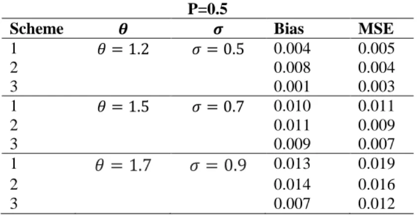
Table 7: Bias and MSE results for different values of 𝜃 and 𝜎. ...41
Table 8: Coverage probability and expected lengths results for different values of 𝜃 and 𝜎 for 𝛼 = 0.1……….42
Table 9: Coverage probability and expected lengths results for different values of 𝜃 and 𝜎 for 𝛼 = 0.05 ...43
Table 10: Bias and MSE results for informative priors ...59
Table 11: Coverage probability and expected lengths results when 𝛼 = 0.1 for informative priors...61
Table 12: Coverage probability and expected lengths results when 𝛼 = 0.05 for informative priors...62
Table 13: Bias and MSE results for different values of 𝜃 and 𝜎 for informative priors ..69
Table 14: Coverage probability and expected lengths results for different values of 𝜃 and 𝜎 when 𝛼 = 0.1 for informative priors ...70
ix
Table 15: Coverage probability and expected lengths results for different values of 𝜃 and
𝜎 when 𝛼 = 0.05 for informative priors ...71
Table 16: Bias and MSE results for noninformative priors ...72
Table 17: Coverage probability and expected lengths results when 𝛼 = 0.1 for noninformative priors...73
Table 18: Coverage probability and expected lengths results when 𝛼 = 0.05 for noninformative priors...74
Table 19: Bias and MSE results for different values of 𝜃 and 𝜎 for noninformative priors ...80
Table 20: Coverage probability and expected lengths results for different values of 𝜃 and 𝜎 when 𝛼 = 0.1 for noninformative priors ...80
Table 21: Coverage probability and expected lengths results for different values of 𝜃 and 𝜎 when 𝛼 = 0.05 for noninformative priors ...81
Table 22: Example 1 (a) confidence intervals for classical statistics methods. ...83
Table 23: Example 1 (b) confidence intervals for Bayesian statistics methods ...84
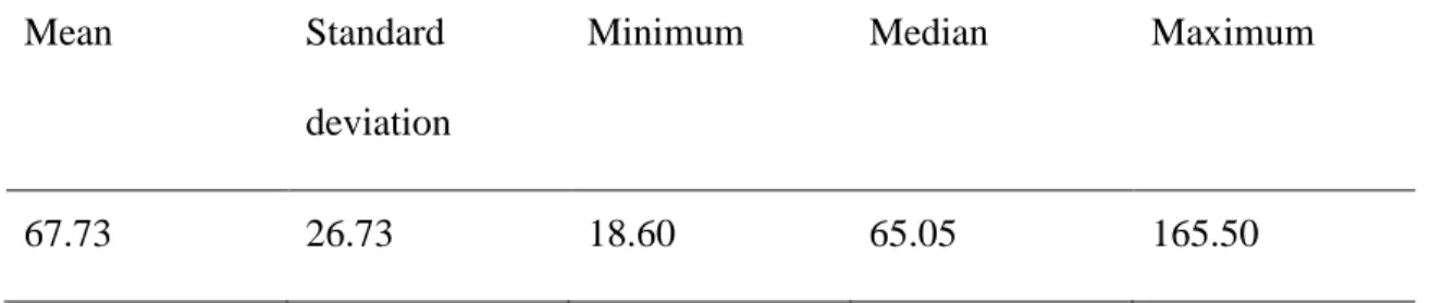
Table 24: Descriptive statistics for the real data. ...87
Table 25: MLEs results of (𝜃, 𝜎, 𝑥𝑝0.1, 𝑥𝑝0.25, 𝑥𝑝0.5, 𝑥𝑝0.75, 𝑥𝑝0.9) parameters. ...90
Table 26: Scheme 1 Confidence Intervals of the classical statistics methods...91
Table 27: Scheme 2 Confidence Intervals of the classical statistics methods...91
Table 28: Bayesian estimates of (𝜃𝐵, 𝜎𝐵, 𝑥𝐵𝑝0.1, 𝑥𝐵𝑝0.25, 𝑥𝐵𝑝0.5, 𝑥𝐵𝑝0.75, 𝑥𝐵𝑝0.9) parameters. ...92
x
xi
LIST OF FIGURES
Figure 1: PDF plot for GE distribution. ...6
Figure 2: Bias and MSE plots for classical statistics methods...36
Figure 3: Expected lengths plots for classical statistics methods when 𝛼 = 0.1 ...37
Figure 4: Coverage probability plots for classical statistics methods when 𝛼 = 0.1 ...38
Figure 5: Expected lengths plots for classical statistics methods when 𝛼 = 0.05 ...39
Figure 6: Coverage probability plots for classical statistics methods when 𝛼 = 0.05. ..40
Figure 7: Bayesian bias and MSE plots for informative priors. ...64
Figure 8: Bayesian expected lengths plots when 𝛼 = 0.1 for informative priors ...65
Figure 9: Bayesian coverage probability plots when 𝛼 = 0.1 for informative priors ....66
Figure 10: Bayesian expected lengths plots when 𝛼 = 0.05 for informative priors ...67
Figure 11: Bayesian coverage probability plots when 𝛼 = 0.05 for informative priors 68 Figure 12: Bayesian bias and MSE plots for noninformative priors. ...75
Figure 13: Bayesian expected lengths plots when 𝛼 = 0.1 for noninformative priors ..76
Figure 14: Bayesian coverage probability plots when 𝛼 = 0.1 for noninformative priors ...77
Figure 15: Bayesian expected lengths plots when 𝛼 = 0.05 for noninformative priors 78 Figure 16: Bayesian coverage probability plots when 𝛼 = 0.05 for noninformative priors ...79
Figure 17: Histogram plot for the real data. ...87
Figure 18: Plot between the expected and the observed distribution...88 *Note to Student: Please note that the capitalization of titles on List of Tables and List of Figures are both acceptable. For example, Page 7 uses Title Case, while page 8 uses Sentence Case. We only ask that you be consistent with your choice throughout the document.
1
CHAPTER 1: INTRODUCTION
In statistical analysis a lifetime or failure time data is wildly used in many areas. Then the lifetime can be defined by having time scale, time origin and an event, which noted as failure or death. In this study we are interested in censored lifetime data especially a progressively type-II censored data. The lifetime data is called censored when an information about an individual survival time is available, but the survival time is not known exactly. The progressively type-II censored data will be approached if the deletions are carried out at an observed failure time. The analysis of this type of data is important in many sciences like the biomedical, engineering, and social sciences. For more explanation, lifetime distribution methodology applications are mainly used to investigate the manufactured items' durability or to study human diseases and their treatment. The interest in analyzing such data is not new. In about 1970, dealing with this type of data had been expanded rapidly depending on methodology, theory, and fields of application. Since about 1980, software packages for lifetime data had been developed widely with a lot of new features and packages.
The lifetime in general is a positive random variable 𝑇 assumed to be continuous with probability density function (pdf) 𝑓(𝑇). Some examples of common lifetime distributions are the exponential distribution, Weibull distribution, log normal distribution, log logistic distribution, and generalized exponential distribution. Censored data occurs when failure times for some units have not been completely observed. There are many causes for censoring. One of these causes is the absence of an event during the study time. If an observation has been lost to follow-up from the study because of death or any other
2
reasons, then this can be a reason for censoring.
In this thesis, we consider the likelihood inference of the quantiles of the Generalized Exponential distribution based on progressively type II censored data. Then, our main research problems are:
1- Investigating and studying the performance of two types of statistical inference, namely; classical inference and Bayesian inference.
2- Considering point estimation as well as interval estimation. Three types of classical confidence intervals have been constructed, namely; the asymptotic interval, the percentile interval, and bootstrap-t interval. For the Bayesian intervals, we considered equal tail intervals as well as the highest probability density (HPD) interval.
3- Comparing between the classical statistical inference point estimation and the Bayesian inference point estimation.
Problems 1, 2, and 3 are presented in chapters 2, 3, and 5, respectively. The rest of this chapter gives a brief explanation and a review of some literature related to our study.
1.1 The Generalized Exponential Distribution
The Generalized Exponential distribution denoted by GE, is a relatively new distribution applied on the life time data. It is introduced by (Gupta & Kundu, Generalized Exponential Distributions, 1999) as a possible alternative for Weibull and Gamma distributions. The main idea of using GE distribution instead of Weibull or gamma distributions is that has the many properties are quite like the gamma distribution, but the distribution function is like the one of Weibull distribution, which will let the computation
3
simpler. The GE distribution is skewed to the right and its monotone hazard function is like the monotone hazard functions of gamma and Weibull distributions. (Khan, 1987) assumed that the GE distribution has two parameters and in case of having an additional parameter which called the location parameter. The GE distribution with an additional parameter fits many situations of life and reliability test results whereas the coefficient of variation of the data is significantly greater than the unity. The GE distribution can be used as an alternative to the Weibull and gamma families for analyzing lifetime data. (Gupta & Kundu, Generalized Exponential Distributions, 1999) presented the distribution function, the probability density function and properties of the distribution. They considered statistical inference techniques for GE distribution.
On the other hand, (Gupta & Kundu, Generalized Exponential Distribution: Statistical Inferences, 2002) derived the maximum likelihood estimation of the unknown parameters of a generalized exponential distribution for both, complete sample and censored sample. They presented the MLEs for both types of censoring, type I and type II. The consistency and the asymptotic normality results of the MLE’s of the GE distribution had been provided by the researchers, in case of complete data. On the other hand, in case of type I censored data and if the data were in grouped form, the Fisher Information matrix had been provided. Also, (Gupta & Kundu, Generalized Exponential Distribution: Existing Results and Some Recent Developments, 2007) assumed that the GE distribution is more useful for analyzing lifetime data than gamma distribution, Weibull distribution or log-normal distribution. They presented the source of this model. Also, some properties and different estimation procedures had been presented. And (Gupta & Kundu, Generalized Exponential Distribution: Bayesian Estimations, 2008) derived the Bayesian estimators for
4
the two unknown parameters of the GE distribution. They assumed gamma distribution as prior distributions for both shape and scale parameters.
This research is based on the generalized exponential distribution. First, we will present the GE distribution with three parameters. A random variable 𝑋 said to be generalized exponential distributed if 𝑋 has the following distribution function
𝐹(𝑥; 𝛼, 𝜆, 𝜇) = (1 − 𝑒−(𝑥−𝜇) 𝜆⁄ )𝛼 (𝑥 > 𝜇, 𝛼 > 0, 𝜆 > 0). (1)
The corresponding density function is
𝑓(𝑥; 𝛼, 𝜆, 𝜇) =𝛼
𝜆(1 − 𝑒
−(𝑥−𝜇) 𝜆⁄ )𝛼−1𝑒−(𝑥−𝜇) 𝜆⁄ (𝑥 > 𝜇, 𝛼 > 0, 𝜆 > 0), (2)
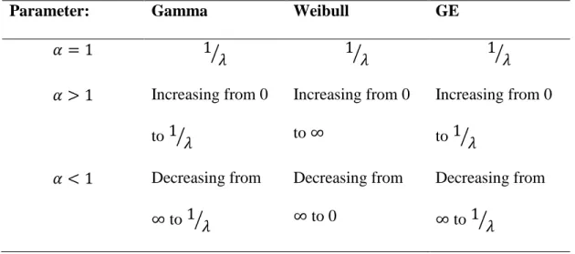
where, the shape parameter is 𝛼, the scale parameter is 𝜆 and the location parameter is 𝜇. The GE distribution can be denoted as 𝐺𝐸(𝛼, 𝜆, 𝜇). The behavior of the hazard function for different values of the shape parameter 𝛼 and its relation with the Gamma and Weibull distributions is explained in the table below.
Table 1. The shape parameter 𝛼 different values.
Parameter: Gamma Weibull GE
𝛼 = 1 1 𝜆 ⁄ 1⁄𝜆 1⁄𝜆 𝛼 > 1 Increasing from 0 to 1⁄𝜆 Increasing from 0 to ∞ Increasing from 0 to 1⁄𝜆 𝛼 < 1 Decreasing from ∞ to 1⁄𝜆 Decreasing from ∞ to 0 Decreasing from ∞ to 1⁄𝜆
5
This research will consider only two parameters. If the location parameter is zero as in most applications of lifetime data models. The shape and scale parameters denoted by 𝜃 and 𝜎 respectively. Therefore, our density and cumulative functions will be defined as follows
𝑓(𝑥; 𝜃, 𝜎) =𝜃 𝜎𝑒
−𝑥 𝜎⁄ (1 − 𝑒−𝑥 𝜎⁄ )𝜃−1 (𝑥 > 0, 𝜃 > 0, 𝜎 > 0). (3)
𝐹(𝑥; 𝜃, 𝜎) = (1 − 𝑒−𝑥 𝜎⁄ )𝜃 (𝑥 > 0, 𝜃 > 0, 𝜎 > 0). (4)
The probability density function proposed in equation (3), has been plotted in the figure below with indicating different parameters sets. These parameters are (𝜃1, 𝜎1) = (2,1.2), (𝜃2, 𝜎2) = (1.2,0.5), (𝜃3, 𝜎3) = (1.5,0.7), (𝜃4, 𝜎4) = (1.7,0.9) and (𝜃5, 𝜎5) = (2.3,1.5).
6
Figure 1.PDF plot for GE distribution.
1.2 Quantiles
Quantiles can be found in many different areas of statistics. It can be applied in many fields like finance, investment, economics, engineering and medicine. The range of a probability distribution can be divided into continuous intervals with equal probabilities by cut points called quantiles. A finite set can be partitioned into q subsets of equal sizes by values called q-quantiles. Historically, there are many uses of sample quantiles in statistics. (Eubank, 1984). In 1846, Quetelet used the probable error of a distribution estimator based on the semi-interquartile range. Also, quantiles like the median had been
7
discussed by (Galton, 1889) , (Edgeworth, Progressive Means, 1886) and (Edgeworth, Review of Fisher's Mathematical Investigations, 1893). Two studies had been made in 1899 by (Sheppard, 1899) and then by (Pearson, 1920) were interested in the problem of choosing the optimal quantile for the mean estimation and the normal distribution’s standard deviation by the subsets of the sample quantiles' linear functions. The asymptotic distribution of the sample quantiles derivation had been discussed in detail in (Pearson, 1920). Simirnoff (1935) explained the behavior of a sample quantile in case of having large sample. Also, he introduced the limiting distribution’s strict derivation. These results had been generalized in 1946 by (Mosteller, 1946), which were supported by (Ogawa, 1951), was highly intentioned with the idea of having quantiles to be an estimation tools in location and scale parameter models. Later, quantiles have been used widely in problems of the classical and the robust statistical inference. Also, quantiles were very important in (Tukey, 1977) and (Parzen, 1979a) works. Which were on the exploratory data analysis and the nonparametric data modeling.
The 𝑝𝑡ℎ quantile for any variable T is the value 𝑡𝑝 such that
Pr(𝑇 ≤ 𝑡𝑝) = 𝑝.
Where, 𝑡𝑝 = 𝐹−1(𝑝). Noticed that, the pth quantile can be referred as the 100 pth percentile
of the distribution. (Pfeiffer, 1990) introduced some properties for the 𝑝𝑡ℎ quantile, which
are shown below:
1- Suppose that the cumulative distribution function 𝐹(𝑥) is continuous and strictly increasing on a closed interval [𝑎, 𝑏], then the 𝑝𝑡ℎ quantile function 𝑡
𝑝 is also
8
2- If the cumulative distribution function 𝐹(𝑥) has a jump at 𝑥 = 𝑎, then the 𝑝𝑡ℎ quantile function 𝑡𝑝(𝑝) = 𝑎 for 𝑝 ∈ (𝐹(𝑎 − 0), 𝐹(𝑎)].
3- If 𝐹(𝑥) = 𝐹(𝑎) for 𝑥 ∈ [𝑎, 𝑏) for 𝐹(𝑎 − 𝑐) < 𝐹(𝑎) and 𝐹(𝑏 + 𝑐) > 𝐹(𝑎), ∀ 𝑐 > 0, then 𝑡𝑝(𝐹(𝑎)) = 𝑎 and 𝑝 > 𝐹(𝑎) implies that 𝑡𝑝(𝑝) ≥ 𝑏.
4- The 𝑝𝑡ℎ quantile function 𝑡
𝑝 is left continuous. For more explanation, the 𝑡𝑝
function is the inverse function of the cumulative distribution function 𝐹(𝑥), then to get the graph of 𝑡𝑝, we may reflect the graph of 𝐹(𝑥) in the main diagonal. By
considering the jump of 𝐹(𝑥) to be a horizontal line. So, the jump of 𝐹(𝑥) will be a horizontal interval for 𝑡𝑝, and a horizontal interval for 𝐹(𝑥) becomes a jump for 𝑡𝑝. Then 𝐹(𝑥) is right continuous and 𝑡𝑝 is left continuous.
5- Suppose that 𝐹(𝑡𝑝(𝑝) − 0) ≤ 𝑝 ≤ 𝐹(𝑡𝑝(𝑝)), therefore if 𝐹(𝑥) is continuous at
𝑡𝑝(𝑝), then 𝐹 (𝑡𝑝(𝑝)) = 𝑝.
1.3 Progressively Censored Data
In statistics, economics, engineering, and medical researches, censoring is a condition where the value of measurement or observation is only partially known. Generally, if the exact survival time is not known, but we have some information about the survival time, in this case the resulting data is said to be censored. Therefore, in survival analysis, time until an event occurs is the variable of interest. The event describes death, disease, or some other individual experience. Survival data has many applications in biomedical science, industrial reliability (for example, reliability engineering, such as lifetime of electronic devices, components, or systems), sociology (for example, period of
9
first marriage), marketing (for example, length of newspaper or magazine contribution), and so on. Now, we review some examples of the survival analysis. Suppose our experiment is about leukemia patients, where the event of interest (failure) is "going out of the reduction" and the outcome is "time in a week until a person goes out of the reduction". The next example is in sociology and it about repetition, where the event is "getting rearrested" and the outcome is "time in weeks until rearrested". As another example, suppose we got a data about transplant patients, the event in this situation is "death" and the outcome is "time in months from receiving a transplant until death".
(Balakrishnan & Cramer, The Art of Progressive Censoring, 2014) As mentioned before, the censored data problem is that the observed data of a variable is partially known. The problem is related to the missing data, where the observed value of some variable is unknown. Therefore, it can be said that the following causes are the reasons of why censoring occurs in the data:
1- There are many reasons that would make a person withdraw the study. 2- During a period of the study, an individual lost to follow-up.
3- No events occur from a person until the study ends.
Theoretically, censoring can be defined as follows. In a life test we usually got n units to test it and a progressive censoring scheme or censoring plan denoted by (𝑅1, … , 𝑅𝑟) . The
units removed from the test within the test period, that process is called progressive censoring in general. There are several models of progressively censored data, but the most popular are the progressive Type-II censoring or the progressive Type-I censoring. The following notations are for progressively censored data.
10
1- 𝑛, 𝑚, 𝑅1, 𝑅2, … ∈ ℕ0 are all integers.
2- The sample size is 𝑚; and for some models, it could be random. 3- The total number of units in the experiment is 𝑛.
4- The effectively employed removals number at the 𝑗𝑡ℎ censoring time is 𝑅j.
5- ℛ = (𝑅1, … , 𝑅𝑟) denoted as the censoring scheme, where 𝑟 is the number of censoring times.
The progressive Type-II censoring is occurred when a surviving unit will be selected randomly to be removed from the experiment when observing a failure to reduce the time and the cost of the experiment.
The set of allowable Type-II censoring schemes can be defined as follows: 𝒢𝑚,𝑛𝑚 = {(𝑟
1, … , 𝑟𝑚) ∈ ℕ0𝑚: ∑𝑚𝑖=1𝑟𝑖 = 𝑛 − 𝑚} .
Suppose we have 𝑘 successive zeros, then the notation for that situation will be 0∗𝑘. In
general (𝑎1, 0∗𝑛1, 𝑎 2, 𝑎3, 0∗𝑛2, 𝑎4, 0∗𝑛3) = (𝑎1, 0, … ,0⏟ 𝑛1 𝑡𝑖𝑚𝑒𝑠 , 𝑎2, 𝑎3, 0, … ,0⏟ 𝑛2 𝑡𝑖𝑚𝑒𝑠 , 𝑎4, 0, … ,0⏟ 𝑛3 𝑡𝑖𝑚𝑒𝑠 ). For
example, (1∗𝑚) means that the censoring scheme (1, … ,1) ∈ 𝒢
𝑚,𝑛𝑚 . The following table
11
Table 2. Different kinds of censoring schemes. Scheme 𝓡 = (𝑹𝟏, … , 𝑹𝒓) Meaning
ℴ𝑚= (0∗𝑚−1, 𝑛 − 𝑚) Right censoring, i.e., the sample size is 𝑛
and the first order statistics are 𝑚.
(0∗𝑚) Complete sample size (𝑚 = 𝑛)
ℴ1 = (𝑛 − 𝑚, 0∗𝑚−1) First-step censoring plan (FSP), i.e., after
failure the exclusion takes place.
ℴ𝑘= (0∗𝑘−1, 𝑛 − 𝑚, 0∗𝑚−𝑘) One-step censoring plan (OSP), i.e., after
the 𝑘𝑡ℎ failure the removal takes place, 2 ≤ 𝑘 ≤ 𝑚 − 1
1.4 Literature on Inference Based on Progressively Censored Data
In this section we shall mention related literature reviews to our study. (Balakrishnan, Progressive Censoring Methodology: An Appraisal (with Discussions), 2007) considered the progressively censored order statistics properties and provided the progressively censored samples' procedures. Basically, he focused in his study on many developments related to this topic. Also, he suggested some problems which further research in future can be. Researcher focused on the progressive Type-II right censoring situation, but he presented a brief idea about Type-I right censoring. He explained the basic distribution theory of the progressively Type-II right censoring. Then he talked about the development of that type of censoring. Three main distributions were interested to apply it
12
for progressively Type-II censored order statistics distribution.
(Sarhan & Abuammoh, 2008) derived the inference procedures for the Generalized Exponential distribution based on a progressively Type-II censored data. They applied Monte Carlo simulation to estimate based on point estimation and the interval estimates. (Ng, Kundu, & Chan, 2009) considered the adaptive Type-II progressive censoring scheme. The maximum likelihood estimation (MLE) has been derived based on the exponential distribution. Also, they constructed the confidence intervals based on diverse methods and applied Monte Carlo simulation to compare their coverage probabilities and expected widths.
(Krishna & Kumar, 2011) obtained the maximum likelihood and Bayesian estimates for one parameter Lindley distribution based on a progressively Type II censored sample. For applications, they used Monte Carlo simulation for calculating interval estimation and coverage probability for their parameter.
(Ye, Chan, Xie, & Ng, 2014) introduced some properties of an adaptive type II progressive censoring. They reduced the bias of the maximum likelihood estimators by using bias correction. After that, they derived the Fisher information matrix for the maximum likelihood estimators of the extreme value distributed lifetimes, considering these properties. To construct confidence intervals for extreme value distribution parameters, they proposed four different approaches. They applied Monte Carlo simulation to compare between these methods. To correct the bias, they used the bootstrap method. The confidence intervals in this study were based on observed information matrix, Fisher information matrix, parametric percentile bootstrap and studentized bootstrap.
13
distribution based on a progressively type-II censored data by using invariance property of MLE after considering the likelihood inference of the GE distribution based on a progressively type-II censored data due to (Sarhan & Abuammoh, 2008). Also, we construct an MLE intervals such as asymptotic, percentile and bootstrap-t confidence intervals due to (Baklizi A. , 2008) and (Baklizi A. , 2009). The new method in this thesis is considering these intervals for the quantiles of the GE distribution based on a progressively censored data. In Chapter 3, we derive the Bayesian inference about the quantiles of the GE distribution based on a progressively type-II censored data due to (Gupta & Kundu, Generalized Exponential Distribution: Bayesian Estimations, 2008) and (Krishna & Kumar, 2011). For simulation study, we apply an importance sampling method. Of course, after constructing confidence intervals for both statistical methods (classical and Bayesian), we calculate the coverage probability and expected lengths of these intervals. Chapter 5 presents a comparison between these two methods considering the bias, mean squared error, coverage probability and expected lengths. Our contributions are that bias and MSE results for Bayesian method are closer to zero more than classical methods. Also, Bayesian intervals have the best expected lengths, especially the equal tail intervals.
14
CHAPTRE 2: LIKELIHOOD INFERENCE
The main idea of the maximum likelihood estimation (MLE) is estimating the parameters of statistical models given observations. (Aldrich, 1997) In 1912, R. A. Fisher derived the “absolute criterion” from the “principle of inverse probability”. The “optimum”, in 1921, was related to the notation of “likelihood” and it was known as a quantity of evaluating hypothetical quantities based on the data given. In 1922, the “maximum likelihood gave estimates which satisfied “sufficiency” and “efficiency”. In that days there were two ways of estimating the likelihood, based on the distribution of the entire sample or sometimes on the distribution of a statistic. Therefore, it could be said that the “Mathematical foundations of theoretical statistics” appeared in 1922 to express the “Maximum likelihood”.
2.1 An Overview of The Likelihood Inference
The maximum likelihood method is based on the likelihood function, which is known as the joint probability distribution or the joint probability density of the random variables 𝑋1, 𝑋2, … , 𝑋𝑛 at 𝑋1 = 𝑥1, 𝑋2 = 𝑥2, … , 𝑋𝑛 = 𝑥𝑛. The likelihood function is
denoted by 𝐿(𝑥; 𝜃) = 𝑓(𝑥1, 𝑥2, … , 𝑥𝑛; 𝜃), where 𝑥1, 𝑥2, … , 𝑥𝑛 are the values of a random
sample from a population with parameter 𝜃. Therefore, the maximum likelihood estimator is found by maximizing the likelihood function with respect to 𝜃, and then we call the value of 𝜃 that maximizes the likelihood function as the maximum likelihood estimate of 𝜃.
We need to find the first partial derivative of the natural logarithm of the likelihood function with respect to 𝜃 to estimate the parameter 𝜃. That first partial derivative is usually called the "score". The Fisher information is given by
15
𝐼(𝜃) = 𝐸 [ 𝜕
2
𝜕𝜃2𝑙𝑛 𝐿(𝑥; 𝜃)] . ( 5 )
Noted that, 0 ≤ 𝐼(𝜃) < ∞. In this study, we may more interested in using the observed Fisher information matrix, which defined as the negative of the second derivative of the log-likelihood function. Therefore, we can say that the Fisher information 𝐼(𝜃) is the expected value of the observed Fisher information matrix.
The invariance property of maximum likelihood estimators is a very useful property. Generally, if a specific distribution has a parameter 𝜃, but suppose the interested estimator is for some function of 𝜃, say 𝜏(𝜃). Formally, a theorem below can express the invariance property of MLEs:
Theorem 2.1.1 (Invariance property of MLEs) (Casella & Berger, 2002) . If the MLE of 𝜃 is 𝜃̂, then for any function 𝜏(𝜃), the MLE of 𝜏(𝜃) is 𝜏(𝜃̂).
Now, we shall define the Asymptotic Normality. Say we have 𝜃̂ is asymptotically normal if
√𝑛(𝜃̂ − 𝜃0) 𝐷
→ 𝑁(0, 𝜎𝜃20) ,
where the parameter 𝜎𝜃02 is known to be the asymptotic variance of our estimator 𝜃̂, while 𝜃0 is known as a true value of parameter 𝜃 . Suppose that 𝜃̂𝑀𝐿𝐸 converges in probability to 𝜃0. Then we say that 𝜃̂𝑀𝐿𝐸 is consistent.
Generally, let a statistical model {𝑓(. , 𝜃): 𝜃 ∈ Θ} of probability density function (pdf) or probability mass function (pmf) on 𝑋 ⊆ 𝑅𝑑 satisfied and in addition to the consistency assumption. Then we have:
16
2- There exists 𝑈 ⊆ Θ, such that function 𝜃 → 𝑓(𝑥 , 𝜃), ∀ 𝑥 ∈ 𝑋 twice continuously differentiable with respect to 𝜃 ∈ U.
3- A 𝑝 × 𝑝 non-singular Fisher information matrix 𝐼(𝜃0) and 𝐸𝜃0[||∇θ𝑙𝑜𝑔𝑓(𝑥, 𝜃0)||] < ∞ satisfies.
4- A compact ball 𝐾 ⊆ 𝑈 of a non-empty interior, exists, which is centered at 𝜃0, such that 𝐸𝜃0𝑠𝑢𝑝𝜃∈𝐾[||∇𝜃
2𝑙𝑜𝑔𝑓(𝑥, 𝜃)||] < ∞ ,
∫x𝑠𝑢𝑝𝜃∈𝐾|∇θ𝑙𝑜𝑔𝑓(𝑥, 𝜃0)|𝑑𝜃 < ∞ ,
∫x𝑠𝑢𝑝𝜃∈𝐾|∇𝜃2𝑙𝑜𝑔𝑓(𝑥, 𝜃)|𝑑𝜃 < ∞ ,
Related to the assumptions above with their properties, then asymptotic normality of the MLE must hold.
Theorem 2.1.2 (Asymptotic normality of the MLE.) Let 𝑋1, 𝑋2, 𝑋3, …, be identically independent distributed (iid) for 𝑓(𝑥|𝜃) and 𝜃̂ be the MLE of 𝜃 . Then,
√𝑛(𝜃̂ − 𝜃0) → 𝑁 (0,
1
𝐼(𝜃0)). ( 6 )
Noticed that, when the Fisher information is larger, then the asymptotic variance of the estimator will be smaller.
Assume that we have a sequence of random variables 𝑇𝑛 such that √𝑛(𝑇𝑛− 𝜃)
𝐷
→ 𝑁(0, 𝜎2) as 𝑛 → ∞ ,
Let 𝑔(𝑥) be a cntinous function such that 𝑔(𝑥) ≠ 0̀ then
√𝑛(𝑔(𝑇𝑛) − 𝑔(𝜃)) 𝐷
→ 𝑁(0, 𝜎2[𝑔(𝜃)̀ ]2).
This result is called the delta method. In the multivariate case, the delta method will be defined as in the following theorem.
17
Theorem 2.1.3 (Multivariate Delta method) (Gugushvili, 2014) Suppose we have a multiparameter vector of differentiated parameters 𝜏 = 𝑔(𝜃1, … , 𝜃𝑘) and it can be differentiated as ∇𝑔 = ( 𝜕𝑔 𝜕𝜃1 ⋮ 𝜕𝑔 𝜕𝜃𝑘) ,
and let 𝜏̂ = 𝑔(𝜃̂). Then 𝜏̂ − 𝜏 → 𝑁 (0, (∇̂𝑔)𝑇𝐼̂−1
𝑛(∇̂𝑔)),
where 𝐼𝑛−1(𝜃) be the inverse of the Fisher information matrix 𝐼𝑛(𝜃), with 𝐼̂−1𝑛 = 𝐼𝑛−1(𝜃̂)
and ∇̂𝑔 = ∇𝑔(𝜃̂).
2.2 The Likelihood Inference
Generally, a data is said to be progressively censored when n items entered in a life time testing experiment and observing m failures. While the first failure is observed an 𝑅1
of the surviving units will be selected randomly and removed. Also, when the second failure is observed, the same thing will be done with an 𝑅2 of the surviving units. Therefore, the experiment will be terminated when mth failures will be observed and all remaining surviving units are removed (i.e, 𝑅𝑚 = 𝑛 − 𝑅1− 𝑅2− ⋯ − 𝑅𝑚−1− 𝑚). The progressively censored sample is denoted as 𝑋1:𝑚:𝑛 < 𝑋2:𝑚:𝑛 < ⋯ < 𝑋𝑚:𝑚:𝑛.
In this research our sample will be progressively type II censored data, therefore the joint density function of 𝑋 = (𝑋1,𝑚,𝑛, … , 𝑋𝑚,𝑚,𝑛) with censoring scheme 𝑅 = (𝑅1, … , 𝑅𝑚) is given by: 𝑓1,2,…,𝑚:𝑚:𝑛(𝑥1, 𝑥2, … , 𝑥𝑚) = 𝑑𝐽(∏ 𝑓(𝑥𝑖:𝑚:𝑛) 𝑚 𝑖=1 ) (∏(1 − 𝐹(𝑥𝑖:𝑚:𝑛)) 𝑅𝑖 𝑚 𝑖=1 )
18
, 0 < 𝑥1:𝑚:𝑛< 𝑥2:𝑚:𝑛 < ⋯ < 𝑥𝑚:𝑚:𝑛 < ∞ , (7) where, 𝑑𝐽 = ∏𝑚𝑖=1[𝑛 − 𝑖 + 1 − ∑max {𝑖−1,𝐽}𝑘=1 𝑅𝑘].
Now, for the generalized exponential distribution, to find the likelihood function of 𝜃 and 𝜎 based on the progressively type II censored data we will substitute equations (3)
and (4) into equation (7) to get:
𝐿(𝑥; 𝜃, 𝜎) = 𝑑𝐽(∏ 𝜃 𝜎𝑒 −𝑥𝑖⁄𝜎(1 − 𝑒−𝑥𝑖⁄𝜎)𝜃−1 𝑚 𝑖=1 ) (∏ (1 − (1 − 𝑒−𝑥𝑖⁄𝜎) 𝜃 )𝑅𝑖 𝑚 𝑖=1 ) , (8)
Taking ln for equation (6) to get:
𝑙𝑛𝐿(𝑥; 𝜃, 𝜎) = 𝑐𝑜𝑛𝑠𝑡 + 𝑚𝑙𝑛𝜃 − 𝑚𝑙𝑛𝜎 −1 𝜎[∑ 𝑥𝑖 𝑚 𝑖=1 ] + (𝜃 − 1) [∑ ln(1 − 𝑒−𝑥𝑖⁄𝜎) 𝑚 𝑖=1 ] + [∑ 𝑅𝑖ln (1 − (1 − 𝑒−𝑥𝑖⁄𝜎)𝜃) 𝑚 𝑖=1 ]. (9)
Now, we need to find the maximum likelihood function estimators for 𝜃 and 𝜎. To do that we must take the first derivative of equation (9) firstly with respect to 𝜃 and then with respect to 𝜎, and then equating each derivative to zero.
𝜕𝑙𝑛𝐿(𝑥; 𝜃, 𝜎) 𝜕𝜃 = 𝑚 𝜃 + ∑ ln(1 − 𝑒 −𝑥𝑖⁄𝜎) 𝑚 𝑖=1 − ∑ 𝑅𝑖 (1 − 𝑒−𝑥𝑖⁄𝜎)𝜃𝑙𝑛(1 − 𝑒−𝑥𝑖⁄𝜎) (1 − (1 − 𝑒−𝑥𝑖⁄𝜎)𝜃) 𝐽 𝑖=1 = 0 , (10) 𝜕𝑙𝑛𝐿(𝑥; 𝜃, 𝜎) 𝜕𝜎 = −𝑚 𝜎 + 1 𝜎2∑ 𝑥𝑖 𝑚 𝑖=1 −(𝜃 − 1) 𝜎2 ∑ 𝑥𝑖𝑒−𝑥𝑖⁄𝜎 (1 − 𝑒−𝑥𝑖⁄𝜎) 𝑚 𝑖=1 + 𝜃 𝜎2∑ 𝑅𝑖 𝑥𝑖𝑒−𝑥𝑖⁄𝜎(1 − 𝑒−𝑥𝑖⁄𝜎)𝜃−1 (1 − (1 − 𝑒−𝑥𝑖⁄𝜎)𝜃) 𝐽 𝑖=1 = 0 , (11)
19
equation by Newton-Raphson method.
The 𝑝𝑡ℎ quantile of GE distribution can be found by finding the inverse function of equation (4) as follows.
𝑡𝑝 = 𝐹−1(𝑝) = −𝜎 log(1 − 𝑝1 𝜃⁄ ). (12)
In our research we are interested in finding the maximum likelihood estimator for the 𝑝𝑡ℎ quantile of GE distribution, which has been found by the invariance property of
MLE by the following equation:
𝑡𝑝(𝜃̂, 𝜎̂) = 𝑥̂𝑝 = −𝜎̂ log(1 − 𝑝1 𝜃⁄̂). (13)
To find the approximate confidence intervals for 𝑥𝑝 for large 𝑚, we need to find the
observed Fisher Information matrix of the parameters 𝜃 and 𝜎, denoted as follows:
𝐽(𝜃, 𝜎) = [ −𝜕2𝑙𝑛𝐿(𝑥; 𝜃, 𝜎) 𝜕𝜃2 − 𝜕2𝑙𝑛𝐿(𝑥; 𝜃, 𝜎) 𝜕𝜃𝜕𝜎 −𝜕 2𝑙𝑛𝐿(𝑥; 𝜃, 𝜎) 𝜕𝜎𝜕𝜃 − 𝜕2𝑙𝑛𝐿(𝑥; 𝜃, 𝜎) 𝜕𝜎2 ] , (14) 𝜕2𝑙𝑛𝐿(𝑥;𝜃,𝜎) 𝜕𝜃2 = −𝑚 𝜃2 − ∑ 𝑅𝑖[ 2(1−𝑒−𝑥𝑖 𝜎⁄ )𝜃𝑙𝑛(1−𝑒−𝑥𝑖 𝜎⁄ ) (1−(1−𝑒−𝑥𝑖 𝜎⁄ )𝜃) + 2(1−𝑒−𝑥𝑖 𝜎⁄ )2𝜃𝑙𝑛(1−𝑒−𝑥𝑖 𝜎⁄ ) (1−(1−𝑒−𝑥𝑖 𝜎⁄ )𝜃) 2 ] 𝐽 𝑖=1 , 𝜕2𝑙𝑛𝐿(𝑥; 𝜃, 𝜎) 𝜕𝜃𝜕𝜎 = − 1 𝜎2∑ 𝑥𝑖𝑒−𝑥𝑖⁄𝜎 (1 − 𝑒−𝑥𝑖⁄𝜎) 𝑚 𝑖=1 +∑ 𝑅𝑖𝑥𝑖𝑒 −𝑥𝑖⁄𝜎 𝐽 𝑖=1 𝜎2 [ (1−𝑒−𝑥𝑖 𝜎 ⁄ )𝜃−1 (1−(1−𝑒−𝑥𝑖 𝜎⁄ )𝜃)+ 𝜃(1−𝑒−𝑥𝑖 𝜎⁄ )𝜃𝑙𝑛(1−𝑒−𝑥𝑖 𝜎⁄ ) (1−(1−𝑒−𝑥𝑖 𝜎⁄ )𝜃) + 𝜃(1−𝑒−𝑥𝑖 𝜎⁄ )2𝜃−1𝑙𝑛(1−𝑒−𝑥𝑖 𝜎⁄ ) (1−(1−𝑒−𝑥𝑖 𝜎⁄ )𝜃) 2 ] ,
20 𝜕2𝑙𝑛𝐿(𝑥; 𝜃, 𝜎) 𝜕𝜎2 = 𝑚 𝜎2− 2 𝜎3∑ 𝑥𝑖 𝑚 𝑖=1 −(𝜃 − 1) 𝜎4 ∑ 𝑥𝑖2𝑒−𝑥𝑖⁄𝜎 (1 − 𝑒−𝑥𝑖⁄𝜎) 𝑚 𝑖=1 −(𝜃 − 1) 𝜎4 ∑ 𝑥𝑖2𝑒−2𝑥𝑖⁄𝜎 (1 − 𝑒−𝑥𝑖⁄𝜎)2 𝑚 𝑖=1 +2(𝜃 − 1) 𝜎3 ∑ 𝑥𝑖𝑒−𝑥𝑖⁄𝜎 (1 − 𝑒−𝑥𝑖⁄𝜎) 𝑚 𝑖=1 −𝜃(𝜃 − 1) 𝜎4 ∑ 𝑅𝑖 𝐽 𝑖=1 𝑥𝑖2𝑒−2𝑥𝑖⁄𝜎𝜃(1 − 𝑒−𝑥𝑖⁄𝜎)𝜃−2 (1 − (1 − 𝑒−𝑥𝑖⁄𝜎)𝜃) + 𝜃 𝜎4∑ 𝑅𝑖 𝐽 𝑖=1 𝑥𝑖2𝑒−2𝑥𝑖⁄𝜎𝜃(1 − 𝑒−𝑥𝑖⁄𝜎)𝜃−1 (1 − (1 − 𝑒−𝑥𝑖⁄𝜎)𝜃) −𝜃 2 𝜎4∑ 𝑅𝑖 𝐽 𝑖=1 𝑥𝑖2𝑒−2𝑥𝑖⁄𝜎𝜃(1 − 𝑒−𝑥𝑖⁄𝜎)2𝜃−2 (1 − (1 − 𝑒−𝑥𝑖⁄𝜎)𝜃)2 −2𝜃 𝜎3∑ 𝑅𝑖 𝐽 𝑖=1 𝑥𝑖𝑒−𝑥𝑖 𝜎⁄ (1−𝑒−𝑥𝑖 𝜎⁄ )𝜃−1 (1−(1−𝑒−𝑥𝑖 𝜎⁄ )𝜃) ,
The inverse of the observed Fisher Information matrix 𝐽−1(𝜃̂, 𝜎̂) would be the asymptotic variance covariance matrix. Which denoted as follows
𝐽𝑛(𝜃̂, 𝜎̂) = 𝐽−1(𝜃, 𝜎)| 𝜃=𝜃̂,𝜎=𝜎̂ = 1 |𝐽(𝜃, 𝜎)| [ −𝜕2𝑙𝑛𝐿(𝑥; 𝜃, 𝜎) 𝜕𝜎2 𝜕2𝑙𝑛𝐿(𝑥; 𝜃, 𝜎) 𝜕𝜃𝜕𝜎 𝜕2𝑙𝑛𝐿(𝑥; 𝜃, 𝜎) 𝜕𝜎𝜕𝜃 − 𝜕2𝑙𝑛𝐿(𝑥; 𝜃, 𝜎) 𝜕𝜃2 ] . (15)
Since, equation (15) is a variance covariance matrix then it is symmetric. Then the asymptotic distribution is as follows
√𝑛 (𝜃̂ − 𝜃 𝜎̂ − 𝜎)
𝑑
→ 𝑁 (0, 𝐽𝑛(𝜃̂, 𝜎̂)), (16)
21 ∇ ̂𝑡𝑝= [ 𝜕𝑡𝑝(𝜃̂, 𝜎̂) 𝜕𝜃̂ 𝜕𝑡𝑝(𝜃̂, 𝜎̂) 𝜕𝜎̂ ] = [ 𝜎̂𝑝1 𝜃⁄̂𝑙𝑛𝑝 𝜃̂2(1 − 𝑝1 𝜃⁄̂) − log(1 − 𝑝1 𝜃⁄̂) ] , (17) Then, √𝑛(−𝜎̂ log(1 − 𝑝1 𝜃⁄̂) + 𝜎 log(1 − 𝑝1 𝜃⁄ )) → 𝑁 (0, ∇̂𝑡𝑝 𝑇 𝐽𝑛(𝜃̂, 𝜎̂)∇̂𝑡𝑝), (18) where, ∇̂𝑡𝑝𝑇𝐽𝑛(𝜃̂, 𝜎̂)∇̂𝑡𝑝 = [ 𝜎̂𝑝 1 𝜃⁄̂𝑙𝑛𝑝 𝜃 ̂2(1−𝑝1 𝜃⁄̂) − log(1 − 𝑝 1 𝜃⁄̂)] [ 𝑣𝑎𝑟(𝜎̂) 𝑐𝑜𝑣(𝜃̂, 𝜎̂) 𝑐𝑜𝑣(𝜃̂, 𝜎̂) 𝑣𝑎𝑟(𝜃̂) ] [ 𝜎̂𝑝1 𝜃⁄̂𝑙𝑛𝑝 𝜃̂2(1−𝑝1 𝜃⁄̂) − log(1 − 𝑝1 𝜃⁄̂) ], = 𝑣𝑎𝑟(𝜎̂) 𝜎̂ 2𝑝2 𝜃⁄̂(𝑙𝑛𝑝)2 𝜃̂4(1 − 𝑝1 𝜃⁄̂)2+ 2𝑐𝑜𝑣(𝜃̂, 𝜎̂) log(1 − 𝑝 1 𝜃⁄̂) 𝜎̂𝑝1 𝜃 ̂ ⁄ 𝑙𝑛𝑝 𝜃̂2(1 − 𝑝1 𝜃⁄̂) + 𝑣𝑎𝑟(𝜃̂)(log(1 − 𝑝1 𝜃⁄̂))2. (19)
We are interested in this study to find the bootstrap estimator of the standard deviation of the maximum likelihood of the 𝑝𝑡ℎ quantile. Generally, the standard deviation is the square root of the variance. Therefore, the square root of equation (19) will be our bootstrap estimator. 𝑆𝐷̂𝑥𝑝 = √𝑣𝑎𝑟(𝜎̂)𝜎̂ 2𝑝2 𝜃⁄̂(𝑙𝑛𝑝)2 𝜃̂4(1 − 𝑝1 𝜃⁄̂)2+ 2𝑐𝑜𝑣(𝜃̂, 𝜎̂) log(1 − 𝑝 1 𝜃⁄̂) 𝜎̂𝑝1 𝜃 ̂ ⁄ 𝑙𝑛𝑝 𝜃̂2(1 − 𝑝1 𝜃⁄̂)+ 𝑣𝑎𝑟(𝜃̂)(log(1 − 𝑝 1 𝜃⁄̂))2 , (20)
22 𝑆𝐷̂̂𝑥𝑝 = √𝑣𝑎𝑟(𝜎̂̂) 𝜎̂̂ 2 𝑝2 𝜃⁄̂̂(𝑙𝑛𝑝)2 𝜃̂̂4𝜃̂̂(1−𝑝1 𝜃⁄̂̂)2+ 2𝑐𝑜𝑣(𝜃 ̂̂, 𝜎̂̂)log(1 − 𝑝1 𝜃̂̂⁄ ) 𝜎̂̂𝑝1 𝜃⁄̂̂𝑙𝑛𝑝 𝜃̂̂2(1−𝑝1 𝜃⁄̂̂)+ 𝑣𝑎𝑟(𝜃̂̂)(log(1 − 𝑝 1 𝜃̂̂⁄ ))2.
The a (1 − 𝛼)% confidence interval for 𝑥𝑝, which based on the asymptotic results that
we got is denoted by
𝑥̂𝑝± 𝑧𝛼 2⁄ 𝑆𝐷̂𝑥𝑝 . (21)
where 𝑆𝐷̂𝑥𝑝 is the asymptotic standard deviation of equation (19) obtained by substituting
𝜃̂ and 𝜎̂.
2.3 Bootstrap Methods
The bootstrap can be considered as an example of modern science in statistics. In 1969, the idea of bootstrap was first proposed by (Simon, 1969). After that, (Efron, 1979a) inspired by the earlier work on the jackknife to publish the bootstrap in "Bootstrap methods: another look at the jackknife". In 1981, a Bayesian extension had been developed.
Bootstrap methods were applied extensively in the literature, (Li, 2011) estimated the interval for the quantiles of two-parameter exponential distributions. He used two methods, bootstrap and fiducial inferences. In his study, he was interested in calculating the coverage probabilities and expected lengths of both methods. He used numerical simulation study for comparing between these two methods. The results showed that fiducial inference method had well performance under all the examined conditions. He applied the Monte Carlo simulation to get coverage probabilities and expected length estimation. The study ended with that coverage probabilities of fiducial intervals were close to 1−∝ and it was larger than the bootstrap intervals for small 𝑝. but for large 𝑝 the
23
coverage probabilities for both methods were close to each other. For that reason, fiducial intervals showed better performance. On the other hand, the expected lengths for bootstrap method showed better results than fiducial method. (Bang & Zhao, 2012) suggested to use censored data to construct confidence intervals by applying some statistical methods such as bootstrap. They did simulation to study the properties of these methods. (Panichkitkosolkul & Saothayanun, 2012) introduced the structure of the bootstrap confidence intervals based on the half-logistic distribution. They applied many types of bootstrap confidence intervals, such as, standard bootstrap, percentile bootstrap and bias-corrected percentile bootstrap confidence intervals. They compared between coverage probabilities and average lengths of bootstrap confidence intervals by using Monte Carlo simulations. The study showed that the coverage probabilities of the standard bootstrap confidence intervals were getting closer to the confidence level than other types of bootstrap confidence intervals. (Baklizi A. , 2008) developed confidence intervals for different quantiles based on one and two independent samples. He considered the maximum likelihood estimator based on record values from the Weibull distribution. He constructed bootstrap-t, bootstrap-t with bootstrap estimated variance and bootstrap percentile intervals and compared between them. This study ended with the length of intervals increased as 𝑝𝑡ℎ quantile values increased. On the other hand, the larger the
sample size the shorter intervals. The error rates were appeared larger for small sample sizes than the nominals. But, for intervals based on the asymptotic normality of the MLE and the observed information matrix or the Fisher information matrix the error rates seems to be moderate. While for all three types of bootstrap intervals, the error rates were very
24
large. (Baklizi A. , 2009) considered the quantiles of the generalized exponential distribution. This study concluded that intervals lengths seems better for higher P values and smaller sample sizes. Intervals' error rates were larger than for nominal ones especially for small sample sizes. While error rates for intervals based on the asymptotic normality of the MLE seemed to be small. Bootstrap intervals, error rates were the largest especially for the percentile interval and the bootstrap-t interval with variance estimates from the Fisher information matrix.
Many journal articles have stressed that bootstrap has great practical value. Also, that journal articles emphasized to consider bootstrapping in applied work. On the other hand, it is not surprising that extremely precise results can be found when combined bootstrapping with modern insights, while traditional methods fail badly. Generally, all bootstrap methods depend on the data has been gotten from a study to detect the sampling distributions, which used to calculate the confidence intervals and test hypotheses. The basic idea of bootstrapping depends on random sampling with replacement. Bootstrapping helps to define sampling distribution of sample means, without considering the normality assumption. It also could assign measures of accuracy (such as variance, bias, confidence intervals, prediction error or some other such measures) to sample estimate. This technique allows by using random sampling method, to estimate the sampling distribution of any statistic. Bootstrap has advantages and disadvantages. The most important advantage is the simplicity of bootstrapping. A standard errors and confidence intervals estimates can be derived easily for complex estimators of complex parameters of the distribution. These complex estimators could be percentile points, odds ratio, proportions, and correlation coefficients. Also, to check the stability and control the results, we can be bootstrapping.
25
On the other hand, bootstrap confidence intervals are asymptotically more precise than the standard intervals, which depend on the sample variance and the normality assumptions. But the simplicity of bootstrapping hides aside of the disadvantage. Which is the fact that important assumptions need to take care of it when bootstrapping, for example independence of samples. There are many methods for bootstrapping. In this study we are interested in bootstrap methods for means, namely the percentile method and the bootstrap t method.
The bootstrap t method arises when we are interested to compute a confidence interval for 𝜇. Suppose the T statistics which is given by
𝑇 = 𝑋̅−𝜇
𝑠 √𝑛⁄ ,
and it has a Student's t distribution. Therefore, the confidence interval for the population mean is given by (𝑋̅ ± 𝑇 𝑠
√𝑛) when sampling from a Normal distribution. The bootstrap t
method or percentile t bootstrap, as it called sometimes, detects the distribution of T. In this situation we get the bootstrap samples same as percentile method, but for this bootstrap sample we must calculate the sample mean and standard deviation, then label them to be 𝑋̅∗ and 𝑠∗.
2.3.1 Bootstrap-t Confidence Interval
To compute the bootstrap-t confidence interval. First, we need to calculate a
vector which is given by 𝑍∗ =(𝑥̂̂𝑝−𝑥̂𝑝)
𝑆𝐷̂̂
𝑥𝑝 , where 𝑆𝐷
̂ ̂
𝑥𝑝 is the estimated asymptotic standard
deviation of 𝑥̂𝑝 and it is defined in equation (20). After that, we need to find 𝑧𝛼∗ which is
26
(𝑥̂𝑝− 𝑧1−𝛼 2∗ ⁄ 𝑆𝐷̂𝑥𝑝, 𝑥̂𝑝− 𝑧𝛼 2∗⁄ 𝑆𝐷̂𝑥𝑝) . (22) 2.3.2 Percentile Confidence Interval
The maximum likelihood estimator of𝑥𝑝 has been introduced in chapter 2 to be 𝑥̂𝑝 as shown in equation (13). Now, we are interested to find the maximum likelihood estimator for the bootstrap samples which generated from the Generalized Exponential distribution with parameters 𝜃̂ and 𝜎̂ . Therefore, by applying the invariance property on equation (13), then 𝑥̂̂𝑝 will be the maximum likelihood estimator for the bootstrap samples.
The percentile confidence interval can be constructed by finding the cumulative distribution function of 𝑥̂̂𝑝 which would be denoted by 𝐻̂ . The 1 − 𝛼 percentile interval for 𝑥̂𝑝 is defined by (𝐻̂−1(𝛼 2) , 𝐻̂ −1(1 −𝛼 2)) . (23) 2.4 Simulation Study
We will investigate the performance of the point and interval estimators. We will consider the bias and MSE for point estimators, the coverage probability and the expected length for confidence intervals.
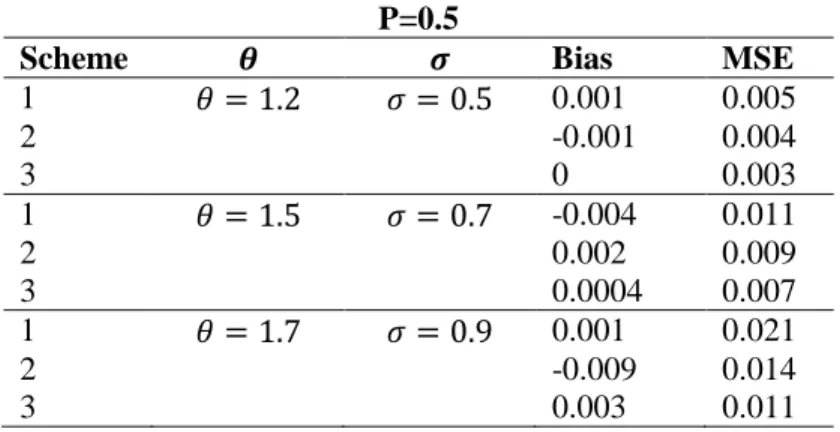
We did simulation for N=2000. Also, we chose different values of P, which cover the whole range of P (0 < 𝑃 < 1). Our parameters values fixed to be 𝜃 = 2 and 𝜎 = 1.2 for table 5. It is important to mention that we choose B=500, which indicates the bootstrap samples for each scheme. Note that the best choice of B to get better results is extremely large. But in this study, we have been chosen the number of bootstrap samples to be B=500. It is noticed that the choice of B is small as (Davidson & MacKinnon, 2001) did. After that we will take
27
other different values of 𝜃 and 𝜎 to check the stability of our results.
This study interested in calculating the bias, the mean-squared error (MSE), and the asymptotic variance. Table 5 shows the results of different estimates replicated 2000 times. For that replication we calculated the following for 𝑥𝑝, 𝑝 = 0.1, 0.25, 0.5, 0.75, 0.9;
1- Bias: The expected value of the difference between the estimator's (𝑥̂𝑝) value and
the true value parameter (𝑥𝑝) is called the bias function of an estimator and it is denoted by:
𝑏𝑖𝑎𝑠 = 𝐸(𝑥̂𝑝− 𝑥𝑝).
2- MSE: Or it called the risk function. It is the expected value of the squared of the difference between the estimator and the true value parameter. MSE measures the quality of an estimator, whenever it is closer to zero, the better. MSE values are always non-negative and it is denoted by:
𝑀𝑆𝐸 = 𝐸(𝑥̂𝑝− 𝑥𝑝) 2
.
After we calculated our parameters, we used it to calculate our confidence intervals. First, we substituted the five different values that we got for 𝑥̂𝑝 into equation (21) to find the asymptotic intervals for all values of P's. We sorted the five vectors of 𝑥̂̂𝑝's before calculating the percentile confidence intervals which noticed in equation (23). To find out the Bootstrap-t confidence interval we calculated first the vector 𝑍∗, which is explained in section 2.3.1, before calculating equation (22) we sorted 𝑍∗ vectors. For both percentile and Bootstrap-t confidence intervals we used "quantile" equation in R software. In this research we are interested in finding the average length and the error rates for each interval
28
we have got. The average length for any confidence interval can be calculated by subtracting the lower bound of the confidence interval from the upper bound. To calculate the error rate for each interval type, we counted how many times that the values of parameter (𝑥𝑝) can be higher than the upper bound or less than the lower bound and then
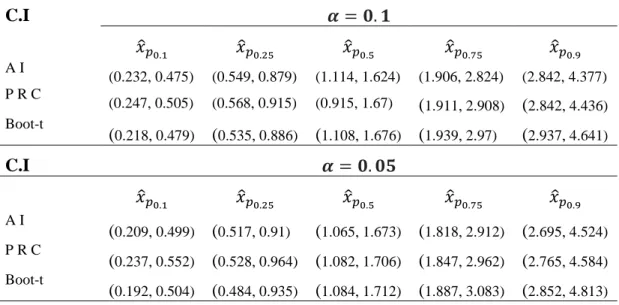
we take the proportion of them to get the error rate. Shortly, we called the confidence intervals in tables 6 and 7 as follows:
1- A I: Asymptotic confidence interval. 2- P R C: Percentile confidence interval. 3- Boot-t: Bootstrap-t confidence interval.
To evaluate the performance of the 𝑝𝑡ℎquantile estimator 𝑥̂
𝑝 and the bootstrap estimator
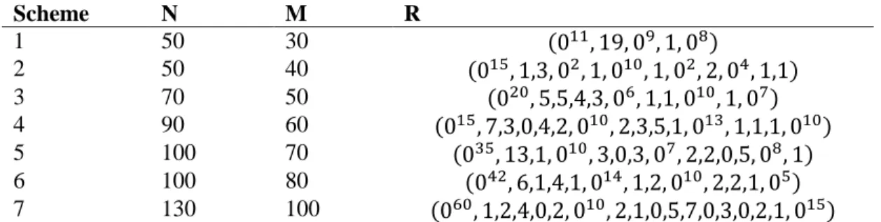
𝑥̂̂𝑝 , we did a simulation study by using R software. To do so, following Mohi El-Din et al. (2016) we chose different censoring schemes with different sample sizes n and different choices of m, where n and m are the total number of units and the sample size, respectively. Table 3 below shows the censoring schemes used in the simulation study.
Table 3. Censoring schemes.
Scheme N M R 1 50 30 (011, 19, 09, 1, 08) 2 50 40 (015, 1,3, 02, 1, 010, 1, 02, 2, 04, 1,1) 3 70 50 (020, 5,5,4,3, 06, 1,1, 010, 1, 07) 4 90 60 (015, 7,3,0,4,2, 010, 2,3,5,1, 013, 1,1,1, 010) 5 100 70 (035, 13,1, 010, 3,0,3, 07, 2,2,0,5, 08, 1) 6 100 80 (042, 6,1,4,1, 014, 1,2, 010, 2,2,1, 05) 7 130 100 (060, 1,2,4,0,2, 010, 2,1,0,5,7,0,3,0,2,1, 015)
29
For generating a progressively type II censored data we used simple simulations steps which had been presented by (Balakrishnan & Sandhu, A Simple Simulational Algorithm for Generating Progressive Type II Censored Samples, 1995) . The following simulation algorithm steps explain the way of generating a progressively censored type II data:
1- Generate 𝑚 independent observations, such that 𝑚~𝑈𝑛𝑖𝑓𝑜𝑟𝑚(0,1). These observations are called 𝑊1, 𝑊2, … , 𝑊𝑚 .
2- Calculate 𝑉𝑖 = 𝑊𝑖1 (𝑖+𝑅𝑚+𝑅𝑚−1+⋯+𝑅⁄ 𝑚−𝑖+1) , ∀ 𝑖 = 1, 2, … , 𝑚.
3- Compute 𝑈𝑖 = 1 − 𝑉𝑚𝑉𝑚−1… 𝑉𝑚−𝑖+1, ∀ 𝑖 = 1, 2, … , 𝑚. Noticed that, 𝑈1, 𝑈2, … , 𝑈𝑚 are required for progressive type II censored sample from Uniform (0,1) distribution.
4- Finally, set 𝑋𝑖 = 𝐹−1(𝑈
𝑖) , ∀ 𝑖 = 1, 2, … , 𝑚. Where the inverse cdf of the
distribution under consideration is known as 𝐹−1(. ). Then the required progressive
type II censored sample from the distribution 𝐹(. ) is 𝑋1, 𝑋2, … , 𝑋𝑚.
Note that, the simulation above needs exactly 𝑚 uniform observations and doesn’t need any sorting.
Before we started our simulation in R software, we downloaded some specific packages in R to make sure that our simulation done perfectly. We will mention some of these packages such as "optimization" and "optimx" to apply the optim function. At the end of the simulation we transferred our results tables to a word document, to do so we downloaded "rtf" and "Rcpp" packages.
30
called optim in R software, but the optim function couldn't find the MLE values directly, so we wrote a command at the end of the function "return(-log_L)", which multiply equation (9) by mines to get our results. Of course, after we got the values of 𝜃̂ and 𝜎̂, we substituted them into equation (13) to get the values of 𝑥̂𝑝's. Also, to find the Fisher
Information matrix, which is defined in equation (5), we included in the optim function a command called "hessian = TRUE". After that we found the inverse of the observed fisher information matrix, noted in equation (15). Then we substituted it in equation (19), which has been calculated directly in R software. Then to find the bootstrap estimator 𝑥̂̂𝑝 , we repeated the optim function using the values of 𝜃̂ and 𝜎̂ that we got for B=500 repeating
this step for N=2000. So, we got the values of 𝜃̂̂ and 𝜎̂̂, and similarly we repeated the steps above to get the values of 𝑥̂̂𝑝's and to find the inverse of the observed fisher information
matrix. After we calculated 𝑥̂𝑝 and 𝑥̂̂𝑝 values, we used it to find what we interested in (Bias
and MSE) as explained above.
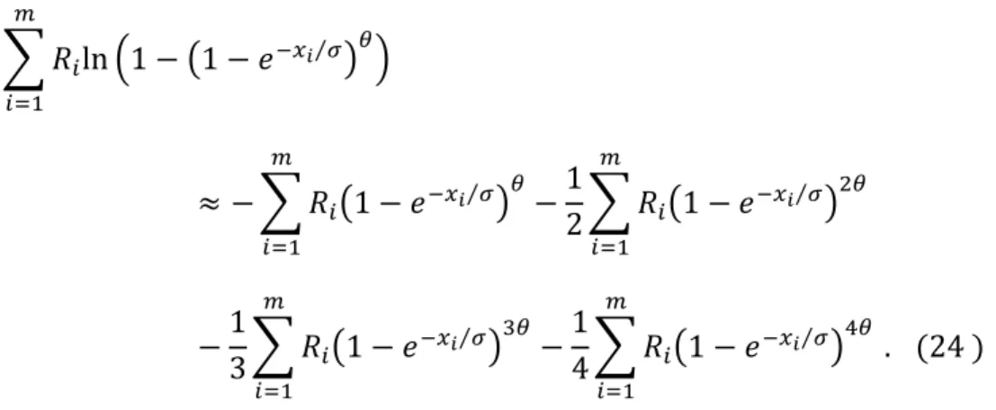
We faced a problem in finding a suitable initial guess. For that reason, we applied an optim function in R software two times. First, we used 𝜃 = 2 and 𝜎 = 1.2 as an initial guess for the first optim function. Also, we applied the Taylor expansion in equation (9). We expanded the following term in equation (9) to be as follows:
31 ∑ 𝑅𝑖ln (1 − (1 − 𝑒−𝑥𝑖⁄𝜎)𝜃) 𝑚 𝑖=1 ≈ − ∑ 𝑅𝑖(1 − 𝑒−𝑥𝑖⁄𝜎)𝜃 𝑚 𝑖=1 −1 2∑ 𝑅𝑖(1 − 𝑒 −𝑥𝑖⁄𝜎)2𝜃 𝑚 𝑖=1 −1 3∑ 𝑅𝑖(1 − 𝑒 −𝑥𝑖⁄𝜎)3𝜃 𝑚 𝑖=1 −1 4∑ 𝑅𝑖(1 − 𝑒 −𝑥𝑖⁄𝜎)4𝜃 𝑚 𝑖=1 . (24 )
Note that we used the first fourth terms of the expansion as an approximation because Taylor expansion likelihood is easy to maximize. After that we used its solution parameters for 𝜃 and 𝜎 as an initial guess for our original likelihood function. Note that, second time we applied the optim function, a Taylor expansion hasn’t been used. We directly used equation (9) for optimizing our parameters.
Table 4. Bias and MSE results for classical statistics methods.
Scheme P=0.1 P=0.25 P=0.5 P=0.75 P=0.9 1 Bias 0.019 0.011 -0.006 -0.031 -0.062 MSE 0.01 0.016 0.037 0.118 0.315 2 Bias 0.017 0.01 -0.004 -0.025 -0.052 MSE 0.01 0.014 0.028 0.083 0.227 3 Bias 0.012 0.007 -0.002 -0.016 -0.033 MSE 0.007 0.011 0.023 0.069 0.182 4 Bias 0.011 0.009 0.003 -0.006 -0.018 MSE 0.006 0.008 0.018 0.057 0.154 5 Bias 0.008 0.004 -0.002 -0.012 -0.022 MSE 0.004 0.007 0.017 0.059 0.165 6 Bias 0.012 0.01 0.004 -0.006 -0.018 MSE 0.005 0.007 0.014 0.039 0.105 7 Bias 0.007 0.005 0.001 -0.003 -0.008 MSE 0.004 0.006 0.013 0.039 0.11
32 In General, the results in table 4 shows that results seem to be slightly similar from one experiment or another, but it is important to note that bias and the MSE, values are lower when we choose larger values of sample sizes 𝑚 and 𝑛 defined in table 3.
On the other hand, it is very clear that values of bias in each scheme is decreasing when increasing the 𝑝𝑡ℎ quantile values. In contrast, mean square error are increased when increasing the 𝑝𝑡ℎ quantile values.
For confidence intervals, we are interested in calculating the interval length and the error rate for each interval. Tables 5 and 6 show the results for intervals lengths and error rates respectively for 2000 replications. On the other hand, confidence intervals are calculated for both 𝛼 = 0.1 and 𝛼 = 0.05 respectively, in tables 5 and 6.
The lengths of all types of intervals can be found by the difference between the upper bound and the lower bound of the intervals. The error rates can be calculated by checking whether the estimator 𝑥𝑝 belongs to the confidence intervals or not.
33 Table 5. Coverage probability and expected lengths results for classical statistics methods when 𝛼 = 0.1 𝜶 = 𝟎. 𝟏 & 𝑵 = 𝟐𝟎𝟎𝟎 Scheme Interval Type P=0.1 P=0.25 P=0.5 P=0.75 P=0.9 A L E R A L E R A L E R A L E R A L E R 1 A I 0.312 0.114 0.395 0.115 0.612 0.12 1.091 0.131 1.788 0.135 P R C 0.315 0.129 0.395 0.114 0.605 0.126 1.071 0.144 1.748 0.15 Boot-t 0.326 0.093 0.413 0.101 0.649 0.112 1.176 0.11 1.952 0.116 2 A I 0.31 0.119 0.381 0.118 0.543 0.107 0.926 0.117 1.509 0.125 P R C 0.327 0.155 0.39 0.126 0.524 0.118 0.84 0.161 1.331 0.192 Boot-t 0.338 0.088 0.417 0.079 0.59 0.096 1.012 0.134 1.674 0.15 3 A I 0.263 0.121 0.328 0.121 0.485 0.118 0.844 0.119 1.382 0.124 P R C 0.265 0.121 0.328 0.121 0.481 0.119 0.834 0.125 1.361 0.131 Boot-t 0.271 0.102 0.337 0.107 0.5 0.109 0.881 0.112 1.452 0.109 4 A I 0.234 0.111 0.294 0.098 0.442 0.099 0.777 0.106 1.273 0.111 P R C 0.235 0.119 0.293 0.104 0.438 0.099 0.769 0.111 1.259 0.115 Boot-t 0.239 0.1 0.3 0.094 0.453 0.099 0.805 0.104 1.328 0.104 5 A I 0.222 0.106 0.275 0.108 0.407 0.107 0.719 0.111 1.186 0.117 P R C 0.229 0.124 0.276 0.113 0.396 0.112 0.678 0.13 1.107 0.145 Boot-t 0.233 0.082 0.287 0.086 0.42 0.104 0.745 0.116 1.241 0.119 6 A I 0.222 0.106 0.273 0.105 0.389 0.108 0.663 0.102 1.082 0.103 P R C 0.227 0.122 0.275 0.118 0.383 0.111 0.643 0.108 1.044 0.111 Boot-t 0.23 0.081 0.2809 0.096 0.396 0.099 0.679 0.099 1.116 0.1 7 A I 0.203 0.109 0.25 0.107 0.363 0.111 0.631 0.116 1.037 0.123 P R C 0.21 0.129 0.254 0.11 0.352 0.116 0.586 0.14 0.946 0.157 Boot-t 0.214 0.086 0.263 0.086 0.375 0.105 0.649 0.138 1.073 0.149
34 Table 6. Coverage probability and expected lengths results for classical statistics methods when 𝛼 = 0.05 𝜶 = 𝟎. 𝟎𝟓 & 𝑵 = 𝟐𝟎𝟎𝟎 Scheme Interval Type P=0.1 P=0.25 P=0.5 P=0.75 P=0.9 A L E R A L E R A L E R A L E R A L E R 1 A I 0.373 0.061 0.474 0.058 0.734 0.069 1.308 0.079 2.144 0.084 P R C 0.376 0.081 0.472 0.069 0.723 0.069 1.28 0.083 2.096 0.086 Boot-t 0.393 0.045 0.5 0.049 0.785 0.058 1.426 0.056 2.369 0.062 2 A I 0.369 0.057 0.455 0.06 0.649 0.063 1.105 0.08 1.803 0.084 P R C 0.388 0.092 0.464 0.072 0.625 0.069 1.001 0.103 1.586 0.124 Boot-t 0.404 0.04 0.501 0.041 0.709 0.051 1.218 0.077 2.014 0.094 3 A I 0.314 0.065 0.392 0.061 0.579 0.062 1.009 0.067 1.652 0.069 P R C 0.316 0.083 0.391 0.072 0.573 0.066 0.995 0.065 1.626 0.068 Boot-t 0.325 0.052 0.404 0.057 0.601 0.06 1.059 0.052 1.75 0.044 4 A I 0.279 0.061 0.351 0.063 0.527 0.063 0.927 0.066 1.519 0.066 P R C 0.28 0.066 0.348 0.065 0.52 0.065 0.912 0.068 1.496 0.066 Boot-t 0.286 0.044 0.358 0.055 0.542 0.055 0.962 0.058 1.59 0.057 5 A I 0.263 0.061 0.325 0.068 0.481 0.057 0.849 0.054 1.401 0.056 P R C 0.271 0.084 0.328 0.075 0.467 0.06 0.801 0.067 1.306 0.072 Boot-t 0.278 0.046 0.34 0.05 0.498 0.056 0.885 0.058 1.476 0.061 6 A I 0.264 0.068 0.326 0.062 0.465 0.06 0.794 0.056 1.297 0.057 P R C 0.27 0.076 0.327 0.067 0.457 0.064 0.767 0.062 1.246 0.064 Boot-t 0.274 0.045 0.336 0.055 0.475 0.056 0.815 0.062 1.342 0.062 7 A I 0.241 0.064 0.298 0.064 0.432 0.058 0.751 0.06 1.233 0.061 P R C 0.25 0.082 0.302 0.068 0.418 0.065 0.696 0.081 1.125 0.09 Boot-t 0.255 0.048 0.314 0.043 0.447 0.058 0.775 0.078 1.283 0.081
Before commenting on tables 5 and 6, we shall describe the coverage probabilities and indicate whether it reach the nominal coverage probability or not? Where the nominal error for 𝛼 = 0.1 and 𝛼 = 0.05 are between 0.08 and 0.12, and between 0.04 and 0.06, respectively. For 𝛼 = 0.1, schemes 1, 2, 3, and 7 don’t attain the nominal coverage probability for some confidence intervals, especially when 𝑝 = 0.75, 0.9. On the other hand, some confidence intervals in table 6 show more problems about attaining the coverage probability, which is clear in all schemes, except scheme 4, and for all 𝑝𝑡ℎ quantiles, except for 𝑝 = 0.5.
35
From tables 5 and 6, we noted that the length of the three types of intervals are getting smaller while taking larger samples ( 𝑚 and 𝑛 are larger which are defined in table 3).
It is very clear that the bootstrap-t interval's lengths are larger than the other intervals, but the smallest one is the percentile interval of the other intervals especially when 𝑝 = 0.5, 0.75, 0.9. That result is more pronounced when 𝑚 and 𝑛 , which are defined in table 3, are larger and in addition when 𝑝 = 0.5, 0.75, 0.9. Also, the average lengths seem to be smaller when 𝛼 = 0.1.
Now, the results for the error rates for each type of intervals. Generally, we can conclude that percentile confidence interval shows more problems in attaining the coverage probability all over the schemes and for all 𝑝𝑡ℎ quantiles. On the other hand, bootstrap-t interval is more likely to attain the coverage probability for all schemes especially when 𝑝 = 0.1 & 0.25.
It is interesting to note that error rates for the three types of intervals are similar from scheme to another and get closer to the nominal probabilities when 𝑚 and 𝑛 are larger. To clarify our results more, we have chosen only four schemes results to plot it by using R software again. Figure 1 presents the plot of the bias and MSE results for schemes 1, 2, 3, and 6. While figures 2 and 4 present the plots of the expected lengths of confidence intervals for the same schemes. Finally, figures 3 and 5 present the plots of these schemes’ coverage probability. It is noted that values of 𝑝 are plotted on the x-access and all the results plotted on the y-access.
36
37
38
39