A Dynamic Analysis of Bid-Ask Spreads with
Multiple Trade Sizes
Han N. Ozsoylev Sa¨ıd Business School
University of Oxford Shino Takayama∗ Department of Economics University of Minnesota May 28, 2005 Abstract
This paper studies how the trade size and the historical sequence of trades affect bid-ask spreads, investors’ trading strategies, and the market maker’s learning process in a multi-period economy. First, we show that there is a nonzero cut-off size below which informed traders never buy or sell, and that larger trade sizes have positive bid-ask spreads, while smaller sizes do not. Then, we prove that the cut-off size decreases stochastically . We also derive the functional relationship between bid-ask spreads and trade sizes and show that bid-ask spreads are monotonically increasing in trade sizes. Moreover, we prove that when additional trade sizes are introduced to the market, the market maker’s learning process can be impaired and the bid-ask spreads for the previously existing trade sizes can vanish under a mild condition. We prove that the smaller trade sizes that do not have a positive bid-ask spread result in zero price change, while for larger trade sizes the rate at which price change increases is a decreasing function of the trade size in all trading periods. Most of our results are broadly consistent with the empirical findings. Others provide testable hypotheses for future studies on the subject.
∗We are grateful to Erzo Luttmer and Jan Werner for their helpful suggestions. Also, we would like to thank Hengjie Ai,
Beth Allen, Marco Bassetto, Camelia Bejan, Florin Bidian, Borys Grochulski, John Rust, Raj Singh, and seminar participants at the University of Minnesota, the 2004 Villa Mondragone Workshop in Economic Theory and Econometrics in Rome for helpful comments. All errors are our own. Corresponding author: Shino Takayama, Department of Economics, University of Minnesota, 1035 Heller Hall, 271-19th Ave South, Minneapolis, MN 55455; e-mail:[email protected].
1
Introduction
Trade sizes, bid-ask spreads, and price changes have been central to the analysis of market microstruc-ture. Empirical market microstructure seeks to characterize the dynamics of prices, bid-ask spreads and trade sizes and has identified a strong link between trade sizes and the absolute value of price change for each trade size (see [14]). The motivation for this paper is to understand how trade sizes affect the dynamics of bid-ask spreads and price changes within the framework of theoretical market microstruc-ture model. The market considered here has a market maker who trades a risky asset with traders and exposes bid and ask prices to traders. The presence of traders with superior information leads to a pos-itive bid-ask spread. A bid-ask spread compensates a market maker for the risk of doing business with the informed traders.
Models of information based bid-ask spreads have been developed by Copeland and Galai [1] and Glosten and Milgrom [10]. In the Copeland and Galai model, the true value of the stock is public information after one trading round. In contrast, in the Glosten and Milgrom model, there are many trading rounds. Orders are assumed to be for one round lot1, and there are two types of traders, either informed or uninformed. Glosten and Milgrom showed that the transaction prices are informative and spreads tend to decline with trade. They finally showed that bid-ask spread vanishes when the trading periods go to infinity.
One of important extensions of Glosten and Milgrom is Easley and O’Hara [6]. They extended Glosten and Milgrom by allowing two trade sizes. In an efficient market, the price of an asset should reflect the true value of the asset. However, empirically, we observe that block trades are made at worse prices than small trades, which is called “block trade premium”, and that there are some asymmetric patterns in trade sizes and the direction of price changes. By allowing two trade sizes, Easley and O’Hara consider block trade premium and shows that under some condition, large trade size is trans-acted at worse price than small trade size. Then, they have tried to find how different an impact of each trade size on price is in two-period model. Easley and O’Hara consider only one and two-period models. Our model generalizes Glosten and Milgrom, and Easley and O’Hara.
The model that we have used is described as follows. As in Glosten and Milgrom [10] and Easley and O’Hara [6], there are three types of agents: a competitive single market maker, informed and uninformed traders. In the beginning of the whole game, Nature chooses the value of the risky asset
1According to [16], we can categorize all trades in stocks on the floors of exchanges into round lots and odd lots based
on the unit of trading. A round lot is one for the unit of trading or some multiple thereof. An odd lot is one for less than the number of shares required for the unit of trading.
and informed traders observe the value. A market maker and uninformed traders do not observe the value. In each round of trades, a trader is randomly selected and comes to the market maker. She learns the market maker’s price-quantity quotes and posts the order quantity and the price at which she will buy or sell the asset. If she is informed, she takes the profit-maximizing quotes. If she is uninformed, she posts the order for her liquidity needs. In this setting, we consider the market maker’s regret-free pricing. Trades occurs sequentially and we analyze movement of the bid-ask spreads over time.
To understand why different trade sizes result in different price changes, consider the following situation. Suppose that there are many trade sizes available for traders and prices of all trade sizes are the same. Then, informed traders would rather trade larger trade sizes than smaller sizes if they know the future payoff of the asset. In this sense, the trade sizes that informed traders trade convey information. After large trades come into the market, the market maker can make an inference concerning the risky payoff of the asset. That is how trade sizes affect future price and impacts of trade sizes on price differ. Notice that in this paper, we consider two different relationship. One is the relationship between trade sizes and price after each trade occurs. The other is the relationship between trade sizes and bid-ask spreads. As the reasons stated above, trade size has an impact on the market maker’s expectation on the risky asset and then the consecutive price. At the same time, since bid-ask spreads also reflect the market maker’s expectation on the risky asset, trade sizes also have a relationship with bid-ask spreads. In the paper, we derive these two functional relationships for empirical tests.
Our model follows the strand of Glosten and Milgrom and Easley and O’Hara, and we extend their models in two dimensions; time and number of trade sizes. The main difference between our model and their models is that we allow multiple (more than two types of) trade sizes in a multi-period economy. Incorporating multiple trade sizes more than two allows us to examine the relationship between more variety of trade sizes and price changes, and to derive this relationship as a function, which is called “price-impact functions”. Moreover, a multi-period model allows us to study the dynamic change of trading behaviors and prices. Our model provides more enriched theoretical framework and testable hypotheses for future research on the subject.
The first contribution of the paper is a description of how trade size affects bid-ask spread, trading behavior and the market maker’s learning process in a dynamic environment where multiple trade sizes are available. More specifically, we show that there is a cut-off size above which the informed traders sell or buy with strictly positive probabilities and larger trade sizes above the cut-off size have positive bid-ask spreads, while smaller sizes do not. Also, we show that the cut-off size decreases when both informed traders and liquidity traders trade in the same way. Interestingly, these results explain how
smaller trade sizes start to have strictly positive bid-ask spreads and we show that it is more likely to happen. In Glosten and Milgrom, bid-ask spreads just decrease. However, our model shows that as trade goes on, smaller trade sizes more likely have strictly positive bid-ask spreads.
In relation with Glosten and Milgrom, we provide some interesting results. We prove that the market maker learns the true value of the asset almost surely when the number of the trading periods is infinity and thus bid-ask spreads eventually vanish almost surely. In addition, we prove that when additional trade sizes are introduced to the market, the market maker’s learning process can be impaired and the bid-ask spreads for the previously existing trade sizes can vanish. In Glosten and Milgrom, the bid-ask spread vanishes as trades occur infinitely. The similar result holds in our model with multiple trade sizes. In addition to this result, we also prove that increasing the number of trade sizes complicates the market maker’s learning process under a mild condition.
The second contribution of the paper is an explanation of the functional relationship between trade sizes and price changes. It becomes possible to describe this functional relationship as price-impact functions only within the model with multiple trade sizes more than two. We provide a theoretical framework for an empirical analysis of price-impact functions. We derive a theoretical price-impact function and prove that the smaller trade sizes that do not have a positive bid-ask spread result in zero price change, while for larger trade sizes the rate at which price change increases is a decreasing function of the trade size in all trading periods. That is, the function displays a concave form in the range of trade sizes which have strictly positive bid-ask spreads. We also show that as trading round goes, the price-impact function becomes flatter. Easley and O’Hara did not have this result because their model was two-period setting.
Our results about a price-impact function coincide with the empirical findings. Hasbrouck [11] and [12] measured a trade’s information effect as the ultimate price impact of the trade innovation. The estimates for a sample of NYSE suggest that the impact is a positive and concave function of the trade size. We show that a theoretical price-impact function derived in our model also displays a concave form and also our result predicts how the price-impact function changes over time. This gives us an interesting testable hypothesis for a future research.
In the paper, we give an explanation of why price change is a concave function of trade sizes using the model with asymmetrically informed traders. Then, we show how curvature of the price-impact function changes along with the information structure. Another important result of the model is that price-impact function that we have derived become flatter as trade goes on. This implies that as more information spreads in a market, the impact of trade sizes on price becomes smaller.
The third contribution is a description of the functional relationship between trade sizes and bid-ask spreads. we derive the relationship between bid-ask spreads and the trade sizes. We show that the bid-ask spreads increases in the trade size. Also, the functional relationship between bid-ask spreads and the trade size shows the concave shape. Easley and O’Hara shows that under some condition, large size has a strictly positive bid-ask spread, while small size does not. We prove that the bid-ask spread increases monotonically in trade size by deriving the functional relationship between the bid-ask spread and trade size.
Most of our results are consistent with the empirical findings. Our results about information based bid-ask spreads coincide with the empirical findings of Glosten [8], which decomposes the bid-ask spread into two parts: one part due to asymmetric information and the other part due to other factors such as inventory costs and shows that the part of the spread due to asymmetric information and the part of the spread due to other factors affect the properties of the transaction-price process differently. Also, by using a maximum likelihood technique, Glosten and Harris [9] find that the asymmetric information component of the bid-ask spread is not economically significant for small trades, but increases with trade size. Our results about a cut-off size and the dynamics of the cut-off size are consistent with their results. Especially, our result shows that larger trade sizes than the cut-off size have strictly positive bid-ask spreads, while smaller sizes do not.
Overall, the paper links the theoretical market microstructure development with empirical work. Although the model still includes the stylized assumptions, the paper provides the following testable hypotheses:
• Information effect on price after small trade size is zero.
• Price change after large trade sizes are transacted has a concave relationship with trade sizes.
• Information component of bid-ask spread monotonically increases in trade sizes.
• Bid-ask spreads in large trade sizes have a concave relationship with trade sizes.
The structure of the paper is as follows. We introduce the model in the second section. In the third section, we provide the equilibrium analysis. In the fourth section, we construct a price-impact function and analyze it. Finally the fifth section concludes.
2
The Model of the Sequential Trades
We consider a model in which potential buyers and sellers trade assets with a competitive market maker. The market maker sets prices at which she will buy or sell any quantity of the traded asset. In our economy, one risky asset is traded for T periods. There is also a risk-free asset with period-T payoff normalized to1. The terminal payoff of the risky asset,V˜, is not known to all agents in the economy. In particular,V˜ ∈ {V , V}with the prior probabilities such that 0 < Pr( ˜V =V) =δ < 1. We assume thatV < V.
There are three types of agents in the economy:
1. risk neutral informed traders, who know the realizationV of the risky asset payoffV˜;
2. liquidity traders, whose trading motives are exogenously determined by a random variable (which will be specified later);
3. a competitive risk neutral market maker, who counter the trade orders made by informed traders and liquidity traders.
The order sizes (quantities) in which the risky asset can be traded are restricted. In particular, the traders can trade the risky asset only in the order sizes which are elements of the set
Ωn={−n, ..., −1,0,1, ..., n}.
In our notation,k and−krepresent purchase and sale of kunits of risky asset, respectively. Ω+n := {1, ..., n}denotes the set of possible purchase order sizes whileΩ−
n := {−n, ...,−1}denotes the set
of possible sales order sizes. The number0represents no trade.
We also assume that the number of informed traders is large enough to make each act competitively. Since informed traders hold the information superiority about the asset value, they have a motivation for trades in order to maximize their expected profit. A market maker trades because there is some chance that she is dealing with an uninformed trader. In addition, bid-ask spreads can compensate her for doing business with informed traders.
Now we will describe how trades actually transpire. TheT-period trading game unfolds according to the following timing structure:
1. In period0, nature chooses the realizationV ofV˜, and all informed traders observeV.
(a) Having observed the trades up to periodt−1, the competitive market maker posts a price for each possible order size;
(b) A new trader (of either informed or liquidity type) arrives at the market and learns the price-quantity quotes of the market maker.
(c) If the trader is informed, she takes the profit-maximizing quote. If the trader is a liquidity trader, she trades in the order size determined by her liquidity needs.
3. In the end of periodT,V becomes public information.
Now we describe the information structure in the market. The type of the trader arriving in period
tis determined by the random variableθ˜twhich takes values in{iv, l}. These letters,iv andl, denote
informed type and liquidity type, respectively. The random variablesθ˜t’s are i.i.d. acrosst= 1, ..., T,
and
Pr(˜θt=iv) =µ, t= 1, ..., T.
If periodttype isl, then the demand is determined by the random variableL˜twith
Pr( ˜Lt=q) =γ(q)>0,
for q ∈ Ωn. The random variables{L˜t}t=1,...,T are mutually independent. The random variablesθ˜t, ˜
Lt, V˜ are mutually independent for all t, as well. We assume that an informed trader, who arrives
at the market once, gets the chance to re-trade with probability0. Thus, an informed trader behaves myopically and ignores the effect of her trade on future periods. The structure of this trading game is common knowledge.
This is the game in which the market maker observes the realized demand at the end of each period. Letqtdenote the order size that the market maker receives in periodt. Thus, eachqtis the action that
is played in periodt. A historyht = (q1, ..., qt)is the realized choices of actions at all periods before
t+ 1. The space of all possiblet-period histories,t≥1, is denoted byΩt n:=
Qt
τ=1Ωn, andhtis taken
to be the generic element ofΩt
n. Also,ht,t≥1, is said to be consistent withhT = (q1, ..., qT) ∈ΩTn
ifhT = (ht, qt+1, ..., qT). For notational convenience, we leth0 = ∅. Letπt : Ωtn−1×Ωn → IRbe a
price function. Then,πt(ht−1, q)denotes the market maker’s price-quantity quote of trade sizeqgiven
ht−1.
Next we define trading strategies of informed traders. The market maker faces a different trader in each period. Since there are multiple trade sizes available and the market maker chooses a price for each quantity, an informed trader may possibly obtain the same profit from trading different sizes. In
this case, the informed trader assigns positive probabilities to those trade sizes (that is, she will take the behavior strategy that assigns positive probabilities to these actions of trading these quantities in an information set).
First, we call as trading strategies a probability functionψ: Ωn→[0,1]such thatPq∈Ωnψ(q) = 1.
We also define support ofψassupp(ψ) :=©q∈Ωn ¯ ¯ψ(q)6= 0ª. We further let ∆(Ωn) := ψ: Ωn→[0,1] ¯ ¯ ¯ ¯ ¯ X q∈Ωn ψ(q) = 1
to be the set of trading strategies. Second, we define a trading strategy of informed traders in each period. In period t, observing the value of V and history ht−1, informed traders choose a trading strategy which assigns a probability distribution over trade sizes in Ωn. Formally, we can define a
trading strategy of informed traders as follows:
Definition 1 A trading strategy of an informed trader in period t prescribes a probability distribution ψt(V, ht−1)∈∆(Ωn)over trade sizes inΩnfor eachV ∈ {V , V}and historyht−1.
Notice thatψt(V, ht−1)assigns a probability that an informed trader trades each quantity. We shall denote the assigned probability to trade a trade sizeq ∈ Ωn byψt(q|V, ht−1). Game theoretically, a collection ofψt(V, ht−1)is a behavior strategy over all trade sizesq∈Ωn.
Next, we consider optimal trading strategy of an informed trader in periodt. Among trading strate-gies, the informed trader chooses the strategy which maximizes her expected profit given the price schedule given by the market maker. In other words, an informed trader which arrives at the market in periodtchooses the trading strategy assigning probability distribution which maximizes her profit.
Definition 2 An optimal trading strategy of an informed trader in period t with respect to πt is a
probability distributionψ∗t(V, ht−1)∈∆(Ωn)over trade sizes inΩnfor eachV ∈ {V , V}and history
ht−1if forπt, ψt∗(V, ht−1)∈arg max ψ∈∆(Ωn) X q∈Ωn ψ(q) [q(V −πt(ht−1, q) )] (1)
Before we proceed, we consider the market maker’s decision problem. She decides each period price schedule based on the history of trade sizes that she has ever received up to the current period and a Bayesian updated belief contingent on each quantity. Our important assumption is that the market maker earns zero expected profits on each purchase and each sale, and she faces no transaction costs. This is a central assumption about a market maker that Glosten and Milgrom [10] and Easley and
O’Hara [6] have used. Competition between market makers leads to such a description. Two market makers are enough to make competition and drive them to zero profit pricing.
To illustrate this, suppose that there are two market makers in this market. Suppose the first market maker put the ask priceA1so that it is strictly greater than her expected value of the asset conditional on her information. Then, the second market maker will choose an ask priceA2 < A1which is greater than the conditional expected value of the asset to attract a trader. Notice that market makers are assumed to be uninformed of the valueV and risk neutral. In each period, an available information set is same for the market makers. Thus, the conditional expected value of the asset will be the same. In this way, the market makers set prices with zero expected profit. We do not explicitly assume the existence of multiple market makers because our focus in the paper is information based bid-ask spreads and as long as zero expected profit pricing is imposed, the result from having multiple market makers is equivalent with one from a single competitive market maker.
We consider how the market maker updates the belief according to each trade size. The market maker sets prices with zero expected profit by using the belief updated after each trade size. In order to move on to equilibrium analysis, we have to specify the market maker’s pricing quotes and thus we need her updating formula. We assume that the market maker is a Bayesian. Now we specify her updating formula.
Take a functionδt: Ωtn→[0,1]. Letδt(ht)denote the probability of risky payoff equal toV given
historyht. From the initial distribution ofV˜, we haveδ0 =δ. Using Bayesian updating, we now have for allq∈Ωn, δt(ht−1, q) := Pr( ˜V =V|ht−1, q) = P Pr( ˜V =V|ht−1) Pr(q|ht−1,V˜ =V) V∈{V ,V}Pr( ˜V =V|ht−1) Pr(q|ht−1,V˜ =V) (2) = P Pr( ˜V =V|ht−1) [µ ψt(q|V , ht−1) + (1−µ)γ(q)] V∈{V ,V}Pr( ˜V =V|ht−1)µ ψt(q|V, ht−1) + (1−µ)γ(q) . (3)
Notice that0 < δ <1andγ(q) >0for allq ∈ Ωn, for allq, the denominator of (3) is non-zero.
Also, following the zero-profit pricing condition, the market maker sets the price equal to
πt(ht−1, q) =δt(ht−1, q)V + (1−δt(ht−1, q))V , ∀ht−1 ∈Ωnt−1,∀q ∈Ωn. (4)
We say that a price functionπtsatisfies the zero-profit pricing condition if the equation (4) holds.
The updating process of the market maker’s belief is summarized in the following (the letter MM means market maker in Figure 1.).
¾ 0 · · · · A trader arrives at the market. ? • The MM quotes πt(ht−1,·). ? • The MM receives the orderqt. ? • The MM updates the beliefδt(ht−1, qt). ? •· · · ·- T
Figure 1. Updating the belief in periodtgiven the historyht−1.
Finally, we define an equilibrium of this game. The equilibrium is defined as a perfect Bayesian equilibrium of the trading game and the zero-profit pricing condition.
Definition 3 An equilibrium consists of a sequence of price functions and optimal trading strate-gies of informed traders, {πt∗, ψ∗t}t=1,2,...,T, and posterior beliefs{δt∗}t=1,2,...,T such that for allt ∈ {1,· · ·, T}, allq∈Ωn, and allht∈Ωtn,
(P1) π∗t satisfies the zero-profit pricing condition with respect toψ∗t(V, ht−1),
(P2) for allV ∈ {V , V},ψt∗(V, ht−1)is an optimal trading strategy in every periodtwith respect to
πt∗, (B) for allq∈Ωn, δt∗(ht−1, q) = Pr( ˜V =V|ht−1) [µ ψt∗(q|V , ht−1) + (1−µ)γ(q)] P V∈{V ,V}Pr( ˜V =V|ht−1)µ ψt∗(q|V, ht−1) + (1−µ)γ(q) . (5)
The condition (P1) implies that the competitive market maker determines the price for each order sizeqsuch that it is equal to the expected value of the risky asset payoff conditional onqand the history of orders. The competition between potential market makers is not explicitly modelled here. Also, since in order to calculate the expected value ofV˜ the market maker uses a updated belief contingent on each order size, the first condition explicitly implies that the belief has to be updated through a Bayesian rule. The condition (P2) means that an informed trader chooses a trading strategy to maximize her profit. Also, note that theT-period historyhT depends on the realization
¡ {θt}Tt=1,{Lt}Tt=1 ¢ of the random vector³{θ˜t}Tt=1,{L˜t}Tt=1 ´ .
The condition (B) specifies the equilibrium belief. The market maker’s belief in equilibrium follows the process defined in (5). For allq ∈ Ωn,(1−µ)γ(q)is non-zero and then the denominator of (5) is
non-zero. Thus, the equilibrium belief path (5) is well-defined.
Notice that since a liquidity trader trades for her liquidity needs, she does not have strategic choices. Therefore, in an equilibrium there is no condition for her strategy to satisfy. Thus, the equilibrium definition above does not include any conditions for her. Actually, the trading game is played between a market maker and an informed trader. The market maker is uninformed and uses a Bayesian rule to update her belief. In this sense, the equilibrium definition has Bayesian game flavor. On the other hand, the market maker uses the zero profit condition for pricing assuming the competition between potential market makers, although this situation is not explicitly modelled. Thus the equilibrium notion that we are using here could be called a (Bayesian) Nash market equilibrium.
Finally, the bid-ask spread of quantity size iis the difference between the ask price of quantity q
and the bid price of the same size. Thus, the periodtbid-ask spread for historyht−1 ∈ Ωtn and order
sizeq∈ {1, ..., n}is formulated as
St(ht−1, q) := πt(ht−1, q)−πt(ht−1,−q).
3
Equilibrium Analysis
3.1 Optimal Trading Strategies of the Informed Traders
Here we analyze the optimal informed trading strategies for given order histories. Our first result shows that if an optimal trading strategy assigns positive probability to a trade size q, all trade sizes larger than q are also assigned positive probabilities. To motivate this result, let us consider an informed trader’s size preference in a uniform-price setting: with a uniform price, the informed trader always prefers to buy the largest trade size if price is lower than the payoff and sells in the largest trade size if price is higher than the payoff. When there is differential pricing, as in our case, informed traders may avoid trading in the largest size with probability one fearing that such a strategy might lead the market maker to hike up the price for that size. As a result, trading that size with probability one would not be profitable for the informed traders.
First, we introduce one proposition about the basic properties of optimal trading strategies. The next proposition is helpful to define an equilibrium. Forπtwhich satisfies (4), the following holds.
1. ψ∗t(0|V, ht−1) = 0∀V ∈ {V , V}.
2. ψ∗t(q|V , ht−1) = 0 ∀q ∈Ω−n.
3. ψ∗t(q|V , ht−1) = 0 ∀q ∈Ω+n.
Proposition 1 implies that an informed trader always trades in non-zero quantities. Also, the in-formed trader sells in caseV = V, and buys in caseV = V. Notice that a sale decreases the market maker’s expectation ofV˜ and a purchase increases it. Also, since(1−µ)γ(q)is always strictly positive in all non-zero trade sizesq, the denominator of (7) is non-zero for all non-zeroq. Notice that there is no liquidity trader who trades0and that the informed trader’s trading zero quantity is of measure zero. So, whenq = 0, the market maker can not obtain any information and so the belief stays the same. In other words, a null order does not affect the market maker’s expectation ofV˜. From these arguments, we can clarify the equilibrium belief as follows:
δ∗t(ht−1, q) = δt∗−1(ht−1) : q= 0 δ∗ t−1(ht−1)[µ ψ∗t(q|V ,ht−1)+(1−µ)γ(q)] δ∗ t−1(ht−1)µ ψ∗t(q|V ,ht−1)+(1−µ)γ(q) : q∈Ω − n δ∗ t−1(ht−1) (1−µ)γ(q) (1−δ∗ t−1(ht−1))µ ψt∗(q|V ,ht−1)+(1−µ)γ(q) : q∈Ω + n. (6)
From (6), for allq∈Ωn,
0< δt(ht)<1, ∀ht∈Ωtn,∀t. (7)
That is, the realization ofV˜ is never fully revealed due to the non-degenerate possibility of liquidity trading at each non-zero order size.
kt(ht−1) = min{k: (1−µ) n X i=k (1− i k)γ(i) + (1−δt(ht−1, qt))µ >0}; (8) kt(ht−1) = min{k: (1−µ) n X i=k (1− i k)γ(−i) +δt(ht−1, qt)µ >0}. (9)
The letters kt(ht−1) orkt(ht−1) are the minimal possible cut-off size above which the informed traders trade with strictly positive probabilities on the long side or the short side, respectively.
Theorem 2 For allht−1 ∈Ωnt−1andt= 1, ..., T, there exists a cut-off sizekt(ht−1)andkt(ht−1)with
kt(ht−1)≥1andkt(ht−1)≥1such thatsupp{ψt∗(V , ht−1)}={kt(ht−1),· · · , n}andsupp{ψ∗t(V , ht−1)}= {−n,· · · ,−kt(ht−1)}.
This simply means that an optimal trading strategy of informed traders isk partially pooling for somekwith1≤k≤n. By Theorem 2 we can classify the types of the optimal trading strategies. DEFINITION. An optimal trading strategy of informed traders,ψt∗, is
• kpartially pooling on the long side if
0 < ψt∗(q|V, ht−1) ≤ 1 for all q ∈ {k, k + 1, ..., n} and ψt∗(q|V, ht−1) = 0 for all q ∈ {0, ..., k−1}.
• kpartially pooling on the short side if
0 < ψ∗t(q|V, ht−1) ≤ 1 for allq ∈ {−n,−n−1, ...,−k} and ψt∗(q|V, ht−1) = 0 for all
q∈ {0, ...,−k+ 1}.
Theorem 2 implies that all optimal trading strategies arekpartially pooling for somek,1≤k≤n. For instance,ψt(i|V, ht−1) = 1, fori < n, cannot occur for anyV and historyht−1. As we will see in Theorem 2, there is a cut-off size beyond which the informed trader never trades with strictly positive probabilities. In this sense, the above classification does include all possible optimal trading strategies.
Notice that as special cases ofkpartially pooling, we have the followings.
• ψ∗t is separating on the long side (short side) ifψt∗ isnpartially pooling on the long side (short side).
• ψ∗t is completely pooling on the long side (short side) ifψt∗is1partially pooling on the long side (short side).
Now, we consider when an optimal trading strategy is separating or pooling. The following three propositions give us a necessary and sufficient condition for each kind of optimal trading strategies. Proposition 3 is about separating, Proposition 5 is aboutkpartially pooling, and Proposition 6 is about completely pooling.
Proposition 3 For allht−1 ∈Ωnt−1andt∈ {1, ..., T},
1. ψ∗t is separating on the long side if and only if V =V and n
n−1 ≥1 +
(1−δt−1(ht−1))µ
γ(n)(1−µ) ; (10)
2. ψ∗t is separating on the short side if and only if V =V and n
n−1 ≥1 +
δt−1(ht−1)µ
This proposition says that as the probability of informed trading goes up, an optimal trading strategy is less likely to be separating. On the other hand, as the probability of informed trading goes down, an optimal trading strategy is more likely to be separating. One interpretation is that if the probability that informed traders trade the largest quantity is high, the market maker puts the very large bid-ask spread in the largest quantity. Then, the informed traders avoid trading the largest quantity and instead trade a different quantity size. In this sense, an optimal trading strategy is less likely to be separating as the probability of the informed trading increases. Reversely, as the probability of the informed trading decreases, an optimal trading strategy is more likely to be separating because the bid-ask spread in the largest quantity is not so large. As a direct corollary to Proposition 3, the following holds.
Corollary 4 In equilibrium, ifµis sufficiently close to0,ψ∗t is separating. On the other hand, ifµis sufficiently close to1,V = V andqt−1 > 0, ψ∗t is not separating in equilibrium. If µis sufficiently
close to1,V =V andqt−1<0,ψ∗t is not separating in equilibrium.
Proposition 5 For allht−1 ∈Ωnt−1andt∈ {1, ..., T},
1. ψ∗t iskt(ht−1)partially pooling on the long side if and only if V =V and (1−µ) n X i=kt(ht−1) µ 1− i kt(ht−1) ¶ γ(i) + (1−δt−1(ht−1))µ > 0, and (12) (1−µ) n X i=kt(ht−1)−1 µ 1− i kt(ht−1)−1 ¶ γ(i) + (1−δt−1(ht−1))µ ≤ 0; (13)
2. ψ∗t iskt(ht−1)partially pooling on the short side if and only if V =V and (1−µ) n X i=kt(ht−1) µ 1− i kt(ht−1) ¶ γ(−i) +δt−1(ht−1)µ > 0, and (14) (1−µ) n X i=kt(ht−1)−1 µ 1− i kt(ht−1)−1 ¶ γ(−i) +δt−1(ht−1)µ ≤ 0. (15)
We can see that the condition (12) for the set of trade sizes which the informed traders trade with the positive probabilities is complement of the condition (13) of the set of trade sizes which the informed traders trade with the probability of zero. The condition for the existence of the partially pooling equilibrium is that there must exist somekabove and beyond which each condition holds. Then, this
kwill be a cut-off size above which the informed traders trade with strictly positive probabilities. As a special case of the above proposition, we obtain the following proposition for a completely pooling equilibrium.
Proposition 6 For allht−1 ∈Ωnt−1andt∈ {1, ..., T},
1. ψ∗t is completely pooling on the long side if and only if V =V and
(1−µ) n X
i=1
(1−i)γ(i) + (1−δt−1(ht−1))µ > 0; (16)
2. ψ∗t is completely pooling on the short side if and only if V =V and
(1−µ) n X i=1
(1−i)γ(−i) +δt−1(ht−1)µ > 0. (17)
In the case of a completely pooling equilibrium, the informed traders trade all possible trade sizes with strictly positive probabilities. Therefore, in the above proposition we do not have condition like (13) in Proposition 5. The similar interpretation stated in Corollary 4 applies here. The first term of (16), (1−µ)Pni=1(1−i)γ(i), is always negative. In order for (16) to hold, the second term, (1−δt−1(ht−1))µ, has to be positive. Therefore, the probability of informed trading,(1−δt−1(ht−1))µ, has to be positive. So, we can say that as the probability of informed trading is greater, an equilibrium is more likely to be completely pooling.
3.2 Existence and Uniqueness of Equilibrium
We have given the necessary and sufficient conditions for the existence of each kind of equilibrium. Before we move on to the analysis of dynamics of these equilibria, we consider whether those equilibria would always exist or different kinds of equilibrium exist simultaneously. The answer is no. The following proposition says that it is always the case that there exists the only optimal strategy of the informed traders in each period.
Proposition 7 For a historyht−1 ∈Ωnt−1,1≤t≤T, an optimal trading strategy of informed traders
ψ∗t is unique.
From Proposition 5, inequalities (12) and (13) or inequalities (14) and (15), we can find a unique
k. In other words, on the long side, a trade size that satisfies both (12) and (13) is a unique cut-off size. For example, when an equilibrium iskpartially pooling,k+ 1makes the right hand sides of (12) and (13) greater than 0 andk−1makes the right hand sides of (12) and (13) smaller than 0. Then, from Lemma 2,ψt∗is determined uniquely (see appendix for details). Therefore, an optimal trading strategy of informed traders is uniquely determined.
Notice that Proposition 7 establishes that there can be no an optimal trading strategy ψt∗ with
ψt(n|V, ht−1) = ψt(−n|V, ht−1) = 0for any V ∈ {V , V}. This means that the informed traders always trade the largest quantity with a strictly positive probability. As the direct corollary to the above proposition, we obtain the unique existence of an equilibrium.
Corollary 8 There exists a unique equilibrium.
The proof is done in the following way. From Proposition 3, Proposition 5 and Proposition 6, we prove that one of the three propositions must hold. Then, we can specify the cut-off size in each period. Thus, there is an optimal strategy. The existence of an equilibrium follows. Notice that the equilibrium consists of the optimal trading strategies and the price function. The price functions are given by the zero profit condition. Given the market maker’s belief, we can determine the price-quantity quotes. As stated in Proposition 7, an optimal strategy is unique. Therefore, the equilibrium exists uniquely. Now we have given the necessary and sufficient conditions for each kind of equilibrium and established the unique existence of an equilibrium. From the point of a game theory, we have specified a behavioral strategy at each node. Also we have shown that a behavioral strategy exists uniquely at each node. The analysis so far is very static in the sense that we focus on period by period condition. Now we turn our attention to the dynamics of the bid-ask spreads in the next section.
3.3 Equilibrium Dynamics
In this section, we consider the market maker’s learning process in the dynamics setting. In order to do so, we will extend the results that we have gotten in the previous section to the multiple periods environment. First, we consider the movement of each kind of equilibrium over time. The following proposition specifies the condition under which the set of trade sizes above which the informed traders trade with strictly positive probabilities expands. In other words, we have specified the condition under which a cut-off trade size decreases over time.
Theorem 9 Let{πt∗, ψ∗t, δ∗t}T
t=1 be an equilibrium. Givenht−1 ∈ Ωtn−1 andht = (ht−1, qt)forqt ∈ Ωn,
1. if ψ∗t is kt(ht−1) partially pooling on the long side and qt > 0, then ψ∗t+1 is kt+1(ht−1, qt)
partially pooling on the long side withkt+1(ht−1, qt)≤kt(ht−1);
2. if ψ∗t is kt(ht−1) partially pooling on the short side and qt < 0, then ψt∗+1 is kt+1(ht−1, qt)
We have known that the cut-off size weakly decreases with a certain probability in each period. In other words, with that probability the cut-off size would not increase. In the next proposition, we consider the conditions under which the cut-off size decreases.
Proposition 10 Let{π∗t, ψt∗, δ∗t}T
t=1be an equilibrium.
1. Suppose that for a historyht−1 ∈Ωnt−1andht= (ht−1, qt)forqt∈Ωn,ψt∗iskt(ht−1)partially
pooling on the long side andqt> kt(ht−1). Thenψt∗+1iskt+1(ht−1, qt)partially pooling on the
long side withkt+1(ht−1, qt)< kt(ht−1)if
δt∗(ht)×( 1 Pn i=kt(ht−1)i γ(i) − 1−µ qtPrt(qt≥kt(ht−1)) ) ≥ 1−µ µ 1 kt(ht−1)×(kt(ht−1)−1) ; (18)
2. Suppose that for givenht−1 ∈ Ωtn−1 andht = (ht−1, qt)forqt ∈ Ωn,ψt∗(V, ht−1)iskt(ht−1)
partially pooling on the short side and qt < −kt(ht−1). Then ψt∗+1 iskt+1(ht−1, qt)partially
pooling on the short side withkt+1(ht−1, qt)< kt(ht−1)if (1−δt∗(ht))×( 1 Pn i=kt(ht−1)i γ(−i) − 1−µ |qt|Prt(qt≤ −kt(ht−1)) ) ≥ 1−µ µ 1 kt(ht−1)×(kt(ht−1)−1) . (19)
Notice that if the condition (18) or (19) does not hold, we will havekt(ht−1) =kt+1(ht−1, qt). One
interpretation of the above proposition is that all trade sizes that the informed traders trade with strictly positive probabilities have bid-ask spreads and then in the next period the informed traders will trade the smaller quantity. As a direct corollary of Theorem 9, we have the following:
Corollary 11 Let{πt∗, ψ∗t, δt∗}T
t=1be an equilibrium.
For a historyht−1∈Ωtn−1andht∈ {(ht−1, q) :q ∈Ωn},
1. if ψt∗ is completely pooling on the long side (short side) and qt > 0(qt < 0), then ψ∗t+1 is
completely pooling on the long side (short side);
2. ifψt∗+1is separating on the long side (short side) andqt> 0(qt <0), thenψt∗is separating on
the long side (short side).
Now we consider the dynamics of the market maker’s equilibrium beliefδt∗. Proposition 3, Proposi-tion 5 and ProposiProposi-tion 6 include endogenous variables,δt∗. The following proposition gives the general
formula of the market maker’s belief and expresses the market maker’s belief with only exogenous variables. We express the market maker’s belief in a recursive way.
For a historyht= (q1, ..., qt)∈Ωtn, let
m+(ht) :={τ :τ ≤t, δτ(hτ)< δτ−1(hτ−1) hτ−1consistent withht},
and
m−(ht) :={τ :τ ≤t, δτ(hτ)> δτ−1(hτ−1) hτ−1consistent withht}.
Letm(ht) = m+(ht)∪m−(ht).In words, m+(ht) denotes the set of periods in which the market
maker’s belief is updated upward andm−(ht)denotes the set of periods in which the market maker’s
belief is updated downward. Moreover,m(ht)denotes the set of periods in which the market maker’s
expectation ofV˜ is non-trivially updated, i.e., it is the set of the periodsτ which satisfies
δτ(hτ)6=δτ−1(hτ−1)
forhτandhτ−1 consistent withht.
Proposition 12 Let{πt∗, ψ∗t, δ∗t}T
t=1be an equilibrium. There exist functionsδt−: Ωnt ×[0,1]→[0,1]
andδ+t : Ωt
n×[0,1]→[0,1]such that for{ht}Tt=1consistent withhT, if|m−(ht)|=∅, thenδt∗(ht) =
δt+(ht, δ)and if|m+(ht)|=∅, thenδt∗(ht) =δ−t (ht, δ)2.
An idea behind Proposition 12 is as follows. In order to derive the market maker’s updated belief in periodt, we first focus on the evolution of the market maker’s belief associated with periods inm+(ht)
and then we consider periods inm−(ht). In other words,δt+gives us the market maker’s belief that is
updated downward given a history and the initial distribution ofδ. In the same way, δt− gives us the market maker’s updated belief that is updated upward given a history and the initial distribution ofδ. A history can be divided into two sets,m+(ht)andm−(ht). A functionδt+(ht, δ)gives us the market
maker’s updated belief associated with periods inm+(ht)whenm−(ht)is an empty set and a function
δt−(ht, δ)gives us the market maker’s updated belief associated with periods inm−(ht)whenm+(ht)
is an empty set. An equilibrium beliefδ∗t(ht)is a combination of these two types of belief because in
general both ofm+(ht)andm−(ht)are non-empty.
Let us describe the relationship between δt∗(ht), and δt+(ht, δ) and δ−t (ht, δ). We consider the
following situation: up to periodt1,m−(ht) is empty and aftert1 up tot2, m+(ht) is empty. Then,
the market maker’s equilibrium belief in periodt1is given byδt+1(ht1, δ), and then the market maker’s equilibrium belief in period t2 is given by δ+t1(ht1, δ
+
t1(ht1, δ)). In a similar fashion, we repeat this procedure up to periodT and obtain a general formula of the market maker’s beliefδt∗(ht).
Now that we know how to obtain the market maker’s belief expressed by only exogenous variables, we combine it with propositions that we have seen in the previous section and see how the initial conditions influence on the optimal trading strategies of the informed traders. The most interesting result is the one applied to Proposition 3. Let|m(ht)|count the number of periods in the setm(ht).
The following proposition describes when informed traders always trade the largest trade size, in other words when the optimal trading strategy in each period is separating. The idea is that since Proposition 3 specifies the necessary and sufficient conditions for an optimal trading strategy to be separating, by substitutingδ∗t derived in Proposition 12, we obtain the following proposition.
Proposition 13 Let{π∗t, ψt∗, δ∗t}T
t=1be an equilibrium.
For a historyht−1∈Ωtn−1andht∈ {(ht−1, q) :q ∈Ωn},
1. ψ∗t is separating on the long side if and only if V =V and n
n−1 ≥1 +
µ
γ(n) (1−µ) +δ(γ(n) (1−µ))|m(ht)|1(γ−(δn) (1−µ)+µ)|m(ht)|−1
,
2. ψ∗t is separating on the short side if and only if V =V and n n−1 ≥1 + µ γ(−n) (1−µ) +δ(1−δ)(γ(−n) (1−µ))|m(ht)| (γ(−n) (1−µ)+µ)|m(ht)|−1 .
An interesting thing about the above proposition is that if n−n1 ≥ 1 + γ(n) (1µ−µ) or nn−1 ≥ 1 + µ
γ(−n) (1−µ), an equilibrium is separating even when the number of periods goes to infinity. The proposi-tion says that if the probability of the informed trading is sufficiently small, an equilibrium is separating. In other words, if the probability of the liquidity trading is sufficiently large compared to the informed trading, an equilibrium is not separating.
3.4 Bid-Ask Spreads and The Market Maker’s Learning Process
So far, we have given the general analysis of the dynamics of an equilibrium. Finally, in this section, we consider the bid-ask spreads. A bid-ask spread in each trade size is defined as the difference between
bid-price and ask-price in each quantity. We will consider the behavior of the bid-ask spreads after the infinitely many transactions in this section.
Notice that:
St(ht−1, q) := (δt(ht−1,−q)−δt(ht−1, q)) (V −V). (20) Bid-ask spread reflects the difference between the market maker’s updated belief after setting the size q and one after buying the size q. Let Kt(ht−1) and Kt(ht−1) denote the maximum and the minimum ofkt(ht−1) andkt(ht−1), respectively. Also, letSt∗(ht−1, q)denote the bid-ask spread in trade sizeqassociated with the equilibrium belief ofδ∗t(ht−1, q)andδt∗(ht−1,−q).
Proposition 14 St∗(ht−1, q) > 0 for all q ∈ {Kt(ht−1),· · ·, n} and St∗(ht−1, q) = 0 for all q ∈ {1,· · ·, Kt(ht−1)−1}.
Proposition 14 implies that the larger trade sizes which informed traders trade with strictly positive probabilities have strictly positive bid-ask spreads, while the smaller sizes do not. An interpretation of Proposition 14 is straightforward. Since the market maker understands which trade sizes the informed traders trade, she assign strictly positive bid-ask spreads in those sizes in order to deal with the informed traders. Proposition 14 explains which sizes have strictly positive bid-ask spreads. Next, we consider when bid-ask spreads for each trade size, even larger sizes, vanish. In order to do so, we first calculate the bid-ask spreads. By substituting the optimal trading strategy derived in Lemma 2 (see Appendix) into (20), we obtain the following lemma:
Lemma 1 Let{πt∗, ψ∗t, δt∗}T
t=1 be an equilibrium. There exists a functionf∗(ht−1,·) : Ωn→ IR such
that for a historyht−1 ∈Ωtn−1,
St∗(ht−1, q) = f∗(ht−1, q)(V −V) (21)
for q= 1, ..., n3.
First, we consider how the bid-ask spread looks like as a function of trade sizes. As we can see from (20), bid-ask spread shows the difference of the market maker’s beliefs after selling and buying the size. Thus we can say that we will consider how this difference changes over the trade sizes. In order to express it, we use the notion of “concavity.” Before we proceed, we define concavity in our setting, because the concavity of functions are usually defined in a continuous domain and our domain is discrete.
Definition 4 A functionSt(ht, q)is defined to be concave in a discrete domain with respect toq if for
allq′ andq′′withq′ < q′′,St(ht, q
′ +m)−St(ht, q ′ )> St(ht, q ′′ +m)−St(ht, q ′′ )for allm∈ N.
Proposition 15 In each interval of[Kt(ht−1), Kt(ht−1)]and[Kt(ht−1), n],St∗(ht, q)is concave in a
discrete domain with respect toq.
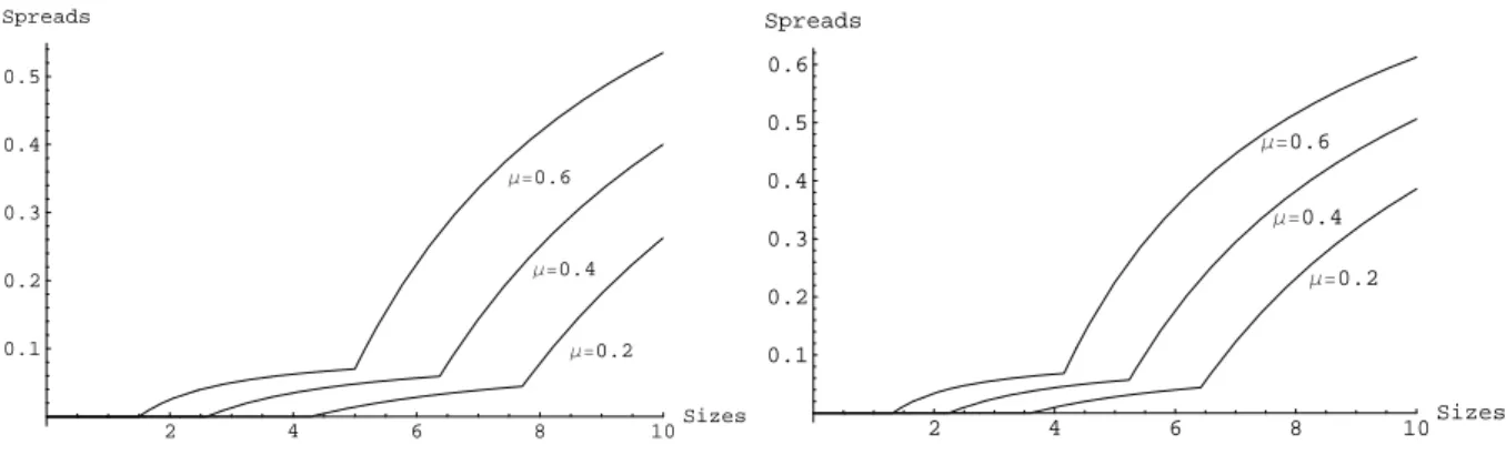
The figure 1 is a continuous representation of the bid-ask spreads functionSt∗(ht−1, q)with respect toq. In the calculation, we have set the market maker’s beliefδ equal to 0.1 and assumed that there are 10 trade sizes available for traders. Also, in the first figure, liquidity traders are assumed to be distributed uniformly over all trade sizes and in the second figure, liquidity traders are distributed with poisson distribution of mean 5, that is γ(q) = 25qq!exp(−5). From the figure, we can see that when the probability of informed trading increases, bid-ask spreads of all quantity sizes become larger. This reflects the market maker’s“risk hedging.” Also, as Proposition 15 says, a continuous representation of
St∗(ht, q)displays concave form in two intervals of[Kt(ht−1), Kt(ht−1)]and[Kt(ht−1), n].
Informed traders are indifferent about trading those sizes in the intervals. Notice that there are two possible equilibrium, long side and short side. The market maker does not know which kind of equi-librium occurs. Therefore, the market maker considers both cases. In a case of long side equiequi-librium, informed traders are indifferent about trade sizes between[kt(ht−1), n]and in a case of short side, in-formed traders are indifferent between trade sizes in[kt(ht−1), n]. It is often the case that these two cut off sizes are different. It is actually the case that as the market maker’s belief changes, these trade sizes change. In this example of Figure 1, the market maker’s beliefδ is0.1. From our calculation, when liquidity traders are distributed uniformly,kt(ht−1) = 8forkt(ht−1) = 5in a case ofµ= 0.2. In other words, whenV =V, informed traders are indifferent about trading sizes above5and whenV = V, informed traders are indifferent about trading sizes above8. The market maker does not know which case is realized. What the market maker knows is that the sizes between5 and8 are transacted only whenV =V and the sizes above8are transacted in either case. That is the reason why there is a kink in the functionSt∗(ht, q)defined inq ∈ {0,· · · ,10}. This is true for the general case for the reasons
explained above.
Notice that the bid-ask spread function for any distribution of liquidity traders displays the simi-lar form. As we explained above, the concave form in the two intervals and the existence of the kink come from the condition that informed traders are indifferent between trading these sizes in each in-terval. When the market maker posts quotes, the market maker considers the distribution of liquidity traders and the informed traders’ trading strategies. For example, as the extreme case, we consider
the situation where almost all liquidity traders sell 9 shares and very few traders trade at other sizes than −9. Informed traders are indifferent between selling the sizes larger than the cut-off size of8 on the short side of the above example. As presented in Lemma 2, (29), if γ(−9) > γ(−10), then
δt∗(−9|V , ht−1)> δ∗t(−10|V , ht−1). However, since the informed traders are indifferent between sell-ing both sizes, it is natural that the change of the market maker’s belief after sellsell-ing the size10 is as much as one after selling the size9.
2 4 6 8 10Sizes 0.1 0.2 0.3 0.4 0.5 Spreads Μ=0.2 Μ=0.4 Μ=0.6 2 4 6 8 10Sizes 0.1 0.2 0.3 0.4 0.5 0.6 Spreads Μ=0.2 Μ=0.4 Μ=0.6
Figure 1: Bid-ask Spreads with Uniformly or Poisson Distributed Liquidity Traders
Corollary 16 Let{πt∗, ψ∗t, δt∗}T
t=1be an equilibrium. Givenht−1∈Ωtn−1andht∈ {(ht−1, q) :q ∈Ωn},
1. St∗(ht−1, n)>0. 2. if n n−1 ≥1 + max ½ µ γ(n) (1−µ), µ γ(−n) (1−µ) ¾ , then St∗(ht−1, q) = 0 forq∈ {1, ..., n−1}.
The first part of the corollary says that there always exists a bid-ask spread in the largest quantity. Since the informed traders trade the largest quantity with a strictly positive probability, it is always the case that a bid-ask spread in the largest quantity is strictly positive. The condition in the second part is from the condition of Proposition 3. The second part says that if a separating equilibrium exists, a bid-ask spread in smaller quantities than the largest size is zero. This is straightforward because if there is no probability that the informed trade these smaller quantities, there is no need for the market maker to put the bid-ask spread. Next, we consider the behavior of the bid-ask spreads when we take the limit of the probability of liquidity trading.
Corollary 17 The followings hold. 1. Asγ(n) +γ(−n)→0,St∗(ht−1, n)→c1 >0. 2. If n n−1 ≤1 + min µ γ(n) (1−µ) +(1−δ)(γ(nδ)(1−µ)+µ) , µ γ(−n) (1−µ) + δ(γ(−n(1)(1−δ−)µ)+µ) ,
then asγ(n−1) +γ(−n+ 1)→pfor some positivep,St∗(ht−1, n−1)→c2 >0.
The first part says that as the probability of informed trading in the largest quantity decreases to0, then the bid-ask spread vanishes. The second part says that as the probability of informed trading in the second largest size converges to some positive probability, the bid-ask spreads in that quantity do not vanish. An interpretation is that when the probability of liquidity trading in the largest trade size is sufficiently small, then the trading in that size will be most probably from the informed traders. Then, we would not have a separating equilibrium because the market maker will put a large bid-ask spread and the informed traders will trade different trade sizes. Therefore, the bid-ask spread in that quantity vanishes as the probability of liquidity trading decreases to zero.
An intuition of the second part is also similar to the first part. Here we have considered the second largest quantity. In a (completely or partially) pooling equilibrium, the informed traders trade the second largest size with a strictly positive probabilities. If there is some probability that a liquidity trading occurs in that quantity, it would be easier for the informed traders to ’hide’ themselves in that quantity and the spreads in the second largest size do not vanish.
So far, we have considered bid-ask spreads across all trade sizes in aT-period game. Now, we turn our attention to bid-ask spreads in the case whereT become sufficiently large. In other words, we study the market maker’s learning process when there are sufficiently large number of trading periods. Before we proceed, we introduce one proposition about when bid-ask spreads for all trade sizes vanish. From (21), the following proposition is straightforward.
Proposition 18 The following holds:St∗(ht−1, q) = 0if and only ifδt∗(ht−1, q) = 0or1forq ∈Ωn.
An interpretation of Proposition 18 is as follows. When the market maker’s belief is 0or1, the bid-ask spreads vanish. In other words, when the market maker learns whether or not the valuation of the asset is high, the bid-ask spreads for all trade sizes vanish. Otherwise, it does not. The result is natural in the sense that when the market maker learns the value of the asset, due to the zero profit
pricing condition, she quote the bid and ask prices of each size at the exactly same level of the value of the asset. Therefore, the bid-ask spreads vanish.
An interesting is that even if the asset is of low value but if the market maker believes that the asset is of high value, the bid-ask spreads vanish. The question here is whether or not this could happen. Else, we would like to know whether or not the market maker learns the value of the asset.
Notice that: for a historyht,
E[δt+1(ht, qt+1)|ht] = E[Pr( ˜V =V|ht, qt+1)|ht] = Pr( ˜V =V|ht)
= δt(ht).
Therefore, the belief δt forms a martingale. An optimal strategy of informed traders prescribes
probability distribution over all trade sizes in each period ofhT and the market maker’s belief assigns a
probability of risky asset’s being equal to the low value in each period given a history up to the period. We consider the market maker’s equilibrium belief as a stochastic process.
Theorem 19 LetT =∞. Then,limt→∞δt(ht) =δ∗almost surely whereδ∗ = 0ifV =V andδ∗ = 1
ifV =V.
The sketch of the proof is as follows. Within the game of an infinitely many periods, we prove that the equilibrium belief converges to some random variable by Martingale convergence theorem. Finally, using the condition for the equilibrium belief, we can show that the random variable takes0ifV =V
and1 ifV = V. Therefore, we can conclude that the market maker finally learns the true value of the asset almost surely. The important thing is that by Corollary 18, the bid-ask spreads vanish almost surely when the number of trading rounds goes to infinity.
3.5 The Number of Trade Sizes and Its Impact on Equilibrium
In this section, we investigate how the number of trade sizes affects bid-ask spreads and the market maker’s learning process. To keep the notation simple, we previously ignored the fact that equilibrium is dependent on the largest trade sizensincenhas been fixed in our analysis till now. We introduce the following notation to carry out the comparative statics required for our investigation: whennis the largest trade size, we let
• {πt,n∗ , ψt,n∗ , δt,n∗ }t=1,...,T denote the equilibrium;
• δt,n(ht)denote the probability of risky payoff being equal to V given the historyht;
• varn(V|ht)denote the variance of risky payoffV conditional on the historyht;
• St,n(ht−1, q)denote the period tbid-ask spread for the historyht−1 ∈ Ωnt−1 and the trade size
q∈ {1, ..., n}.
If the market regulators add new trade sizes to the economy, how would this affect the bid-ask spreads for the previously existing trade sizes? This is the first question that we investigate in this section. Our analysis introduces new trade sizes by increasing the largest trade size n. We see that if sufficiently high number of new trade sizes are introduced into the economy and the probability of liquidity trading in these new sizes is high enough then the bid-ask spreads for the previously existing trade sizes vanish. Formally, we have the following:
Proposition 20 Let{π∗t,n, ψt,n∗ , δt,n∗ }t=1,...,T be the equilibrium, given the largest trade sizen∈ {1,2, ...}.
Supposelimn→∞Pni=1iγn(+i) = limn→∞Pni=1iγn(−i) = ∞. For any given trading periodt≥1
and history(ht−1, q)∈Ωtm, there existsN(ht−1,q) ∈ {m+1, m+2, ...}such that for allm ′≥N
(ht−1,q) 0 = St,m∗ ′(ht−1, q) ≤ St,m∗ (ht−1, q).
The inequality above becomes strict if ψt,m∗ (V, ht−1, q)is non-zero for someV ∈ {V , V}.
The key to this result lies in the following observation. If pricing were uniform, informed traders would choose to trade in the largest available trade size since they can reap the highest profit by doing so. In anticipation of such behavior, the market maker puts a spread between the bid and ask prices of the large trade sizes, which compensates her for the risk of doing business with informed agents. Naturally, the spread for any given trade size decreases as the probability of liquidity trading in that size increases, because such an increase means lower risk of trading with informed traders. When the probability of liquidity trading in large trade sizes is high enough, spreads shrink and informed traders prefer to trade in these large quantities. Introducing new trade sizes by increasing the largest trade size
nessentially means adding larger trade sizes to the economy. If the number of these new and large trade sizes is sufficiently large and the probability of liquidity trading in these new sizes is sufficiently high, informed traders will trade in these new sizes and they will no more trade in the previously existing trade sizes. Since there is no more risk of doing business with informed traders in the previously existing trade
sizes, these trade sizes will have no spreads between their bid and ask prices. Hence we have the result stated in Proposition 20.
Proposition 20 guarantees a high probability of liquidity trading in the newly introduced large trade sizes by imposing the condition
lim n→∞ n X i=1 iγn(+i) = lim n→∞ n X i=1 iγn(−i) = ∞.
This condition is satisfied, for instance, by the sequence of probability functions, {γn}∞n=1, which uniformly distributes liquidity trading over the trade sizes inΩn. This is the sequence,{γn}∞n=1, with
γn: Ωn→[0,1]andγn(i) = 2n1+1, ∀i∈Ωn.
Next we investigate how the introduction of new trade sizes affects the market maker’s learning process. We measure the effect of a trade, in the sizeq and periodt, on the market maker’s learning process by the precision of risky payoff V conditional on her information and the knowledge that
q will be traded in that period, which is var(V|1h
t−1,q). So, the higher this conditional precision, the market maker’s learning process improves, and the lower this conditional precision, the learning process gets impaired. The following proposition shows that introducing new trade sizes by increasing the largest trade sizencan actually impair the market maker’s learning process for trades occurring in the previously existing trade sizes.
Proposition 21 Let{πt,n∗ , ψ∗t,n}t=1,...,T be the equilibrium, given the largest trade sizen∈ {1,2, ...}.
Supposelimn→∞Pni=1iγn(+i) = limn→∞Pni=1iγn(−i) = ∞. For any given trading periodt≥1
and history(ht−1, q)∈Ωtm, there existsN(ht−1,q) ∈ {m+1, m+2, ...}such that for allm ′≥N (ht−1,q) 1.varm′(V|ht−1, q)≥varm(V|ht−1, q) if δ≤ 1 2, and(ht−1, q)∈(Ω+m∪ {0}) t , 2.varm′(V|ht−1, q)≥varm(V|ht−1, q) if δ≥ 1 2, and(ht−1, q)∈(Ω−m∪ {0}) t .
The inequalities above become strict if ψ∗t,m(V, ht−1, q) is non-zero for some V ∈ {V , V}, in
addition to the conditions stated above.
It is easy to check that all results in this paper hold when the space of trade sizes is taken as
½ 1 n, 2 n, ..., n−1 n ,1 ¾ .
Therefore, our analysis also allows us to investigate the implications of policy to introduce smaller trade unit in a stock market, that is, we can see the impacts of trading in smaller increments of stock numbers. The analysis above shows that this institutional change can cause bid-ask spreads to vanish and market maker’s learning process to be impaired when orders are made in small trade size.
4
The Price-Impact Function
In this section, we consider the relationship between trade sizes and the expected price changes condi-tional on each trade size. This relationship is formed as a price-impact function. We define the function as:
Rt(ht−1, q) =πt(ht−1, q)−πt−1(ht−1). (22) The functionRt(ht−1, q)shows the expected change of price conditional on trade sizeqgiven the historyht−1 in periodt. We can rewrite (22) as:
Rt(ht−1, q) = (δt−1(ht−1)−δt(ht−1, q))(V −V). (23) For a simplicity of calculation, we supposeV −V = 1. Notice that forq >0,Rt(ht−1, q)≥0and forq < 0,Rt(ht−1, q) ≤ 0. We also denote the price-impact function in periodtafter a historyht−1 determined by the equilibrium variables byR∗t(ht−1, q)for eachq∈Ωn.
Proposition 22 Let{π∗t, ψt∗, δt∗}T
t=1 be an equilibrium and suppose that we havektpartially pooling
equilibrium on either the long side or the short side. For allq ≤ kt,R∗t(ht, q) = 0.For allq > kt,
Rt∗(ht, q)is concave in a discrete domain with respect toq.
Proposition 22 says that among all trade sizes with strictly positive bid-ask spreads, in other words, larger than the cut-off size, the increment of price change decreases as trade sizes increase. Since trade sizes take on only integers, we do not explicitly use the words,“concave.” However, we can say that the approximated continuous function of the price-impact function displays a concave form.
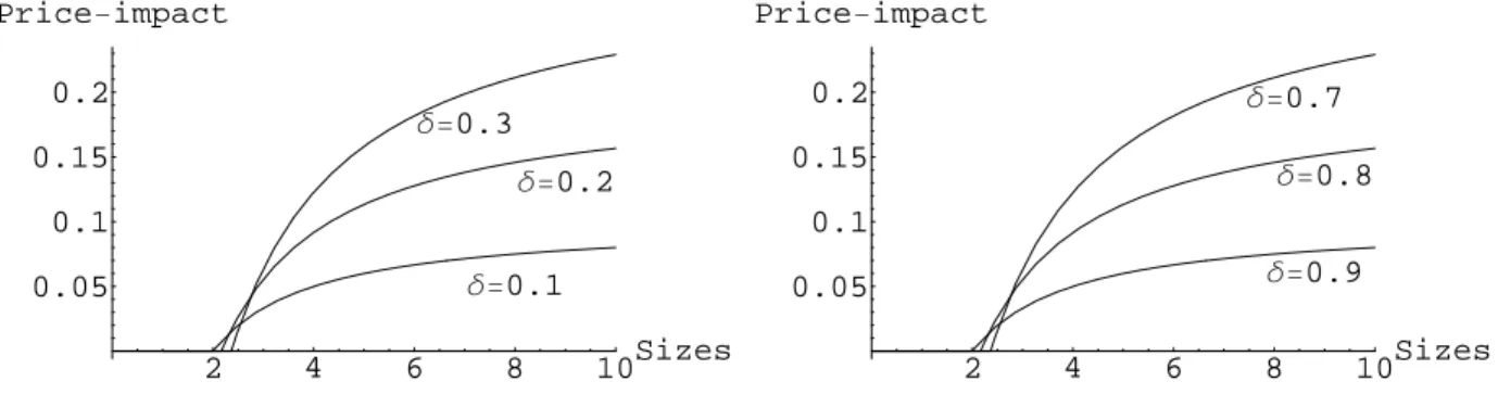
Here, we have some numerical examples of the price-impact functions. Takeµ= 0.5andn= 10. The Figure 1 shows the price-impact function in the case whereγ(q) = 21n. The first figure shows the function on the long side and the second one shows the function on the short side. Notice that trade sizes can take on only integers. That is, the liquidity traders are distributed uniformly. In this figures, we connected those points to approximate the functional form. The Figure 2 shows the price-impact function in case whereγ(q) = 25qq!exp(−5). That is, the liquidity traders are distributed with poisson distribution of mean5.
In the following figures, we plot |R∗t(ht−1, q)| over all quantities. In both figures, points which intersects withx-axis are cut-off sizes. We can see that the cut-off size decreases asδdecreases on the long-side or asδincreases on the short-side. Also, we can see that after the cut-off size, the price impact takes on a concave functional form and that is why in a small quantity just after the cut-off size, change in impact is large.
2 4 6 8 10Sizes 0.05 0.1 0.15 0.2 Price-impact ∆=0.3 ∆=0.2 ∆=0.1 2 4 6 8 10Sizes 0.05 0.1 0.15 0.2 Price-impact ∆=0.7 ∆=0.8 ∆=0.9
Figure 2: Price-impacts with uniform distributed liquidity traders
2 4 6 8 10Sizes 0.05 0.1 0.15 0.2 Price-impact ∆=0.3 ∆=0.2 ∆=0.1 2 4 6 8 10Sizes 0.05 0.1 0.15 0.2 Price-impact ∆=0.7 ∆=0.8 ∆=0.9
Figure 3: Price-impacts with poisson distributed liquidity traders
5
Concluding Remarks
The old adage of Wall street says that “it takes volume to move prices”. The paper sheds light on the relationship between trade sizes and prices in a dynamic model. In a market with asymmetrically in-formed agents, trade sizes that inin-formed traders trade convey information and therefore cause impacts on the security price. The impacts of trade sizes on price differ. It is important to understand what is the relationship between price change and trade size. For this purpose, this paper gives the enriched the-oretical framework of the canonical model Glosten and Milgrom [10] and provide testable hypotheses for future studies on the subject.
Our main results are as follows. We have shown that there is a nonzero cut-off size above which informed traders possibly buy or sell, and that larger trade sizes have positive bid-ask spreads, while smaller sizes do not. Then, we have proved that the cut-off size decreases if both informed traders and liquidity traders trade in the same way. Moreover, we have proved that when additional trade sizes are