Distributed Anomaly Detection using Minimum
Volume Elliptical Principal Component Analysis
Colin O’Reilly,
Member, IEEE,
Alexander Gluhak and Muhammad Ali Imran,
Senior Member, IEEE
Abstract—Principal component analysis and the residual error is an effective anomaly detection technique. In an environment where anomalies are present in the training set, the derived principal components can be skewed by the anomalies. A further aspect of anomaly detection is that data might be distributed across different nodes in a network and their communication to a centralized processing unit is prohibited due to communication cost. Current solutions to distributed anomaly detection rely on a hierarchical network infrastructure to aggregate data or models, however, in this environment links close to the root of the tree become critical and congested. In this paper, an algorithm is proposed that is more robust in its derivation of the principal components of a training set containing anomalies. A distributed form of the algorithm is then derived where each node in a network can iterate towards the centralized solution by exchanging small matrices with neighbouring nodes. Experimental evaluations on both synthetic and real-world data sets demonstrate the superior performance of the proposed approach in comparison to principal component analysis and alternative anomaly detection techniques. In addition, it is shown that in a variety of network infrastructures, the distributed form of the anomaly detection model is able to derive a close approximation of the centralized model.Index Terms—anomaly detection, outlier detection, principal component analysis, distributed learning
F
1
I
N T R O D U C T I O NCentralized learning, where the data set is available in its entirety to one classifier, is a well-studied area. However, if the data set is distributed over more than one physical location, a different approach needs to be taken. For the centralized approach, this requires the communication of all data to a central node, which can be prohibitive if the data set is large. Robustness is also reduced as links close to the central node become critical. A local learning ap-proach uses the data set in the local location to construct a classifier, this has the advantage that no communication between nodes is required. However, insufficient data might mean that the classifier is not representative of the whole data set, and different nodes will form different models. An alternative approach, distributed learning, aims to allow communication between nodes in order for nodes to construct a classifier that tends towards the centralized model. Nodes communicate summarized information about the local data set, with this being used to construct a global classifier on each local node.
1.1 Motivation
Anomaly detection, also known as outlier detection, is a machine learning problem. An anomaly is defined by Barnettet al.as “an observation (or subset of observations)
We acknowledge the support from the REDUCE project grant (No. EP/I000232/1) under the Digital Economy Programme run by Research Councils UK – A cross-council initiative led by EPSRC.
C. O’Reilly, and M. A. Imran are with the Institute for Communica-tion Systems (ICS), Faculty of Engineering and Physical Sciences, Univer-sity of Surrey, Guildford, GU2 7XH, United Kingdom (e-mail: {c.oreilly, m.imran}@surrey.ac.uk).
A. Gluhak is with Digital Catapult, 101 Euston Rd, London NW1 2RA, United Kingdom (e-mail: [email protected]).
which appears to be inconsistent with the remainder of the data” [1]. Anomaly detection aims to identify data that do not conform to the patterns exhibited by the data set [2]. Methods often use an unsupervised one-class one-classification approach. The problem thus has two important characteristics, the data are not labelled and there is a class imbalance in the training set where the number of normal data significantly exceeds the number of anomaly data.
The nature of sensor, peer-to-peer and ad hoc wireless networks requires a distributed learning approach, as it is infeasible to communicate all data to a centralized node for computation. There are several reasons why data might be in different physical locations.
• The data set is too large to transfer to one physical
location. Examples include domains where there are large high-resolution images such as medicine and astronomy.
• It is too costly to transfer the data to one physical
location. Examples include limited energy resources, such as in Wireless Sensor Network (WSN)s, and limited time resources, such as in network intrusion.
• The owners of the distributed data sets are unwilling
to share the data, but require knowledge from the whole data set i.e. there are data ownership and control issues. Examples include data sets containing sensitive information such as medical data sets. It also includes different organizations in areas such as insurance and banking where the data are com-mercially sensitive, but knowledge is required from the whole data set.
1.2 Contribution
In this paper, a distributed anomaly detection scheme based on the principal component analysis (PCA) and the soft-margin minimum volume ellipse is proposed. The approach addresses the challenge of performing anomaly detection in a network where the only assumption is that it is strongly connected, whereas previous research has focused on hierarchical networks, for example [3], [4]. In addition, a modified version of PCA based on the soft-margin minimum volume ellipse is derived, which is robust to anomalies in the training set. Previous ap-proaches have also used the minimum volume ellipse [5]. The proposed approach requires the solution of a convex optimization problem, which allows the distributed form of the algorithm to be derived.
State of the art is extended in the following way:
• A robust version of PCA based upon the soft-margin
minimum volume ellipse is introduced. This im-proves on the performance of classical PCA when there are anomalies in the training set.
• A distributed version of the robust PCA algorithm
is introduced. The algorithm operates in a fully distributed manner that does not require learning on a centralized node and only assumes that the network is strongly connected.
• A detailed evaluation of anomaly detection in a
distributed environment is provided. The proposed technique is evaluated with synthetic and real-world data and compared with other state-of-the-art meth-ods.
1.3 Related Work
There are two approaches to learning in a distributed en-vironment. The first assumes a structure to the network, i.e. assumptions are made concerning the connectivity graph Gand this is exploited during learning. We term thispartially distributedlearning. An alternative approach is to make no assumptions concerning the structure of the network. An algorithm isfully distributedwith respect to a network connectivity graphGif each node operates without using any information other than knowledge of its local neighbourhood inG[6].
Partially distributed learning algorithms often use a hierarchical tree-structure where data or models from child nodes are aggregated or merged at parent nodes. At the root, the global model is constructed, and this is then propagated through the network by communicating the global model to child nodes. There are many examples of partially distributed learning using various anomaly detection methods in a one-tier hierarchical network [7], [8] and a multi-tier hierarchical network [3], [4]. However, the use of the hierarchical tree-structure has several drawbacks. The hierarchical tree-structure means that the links further up the tree become critical and possible bottlenecks. In addition, although the hierarchical tree-structure assumes that it is one-hop between nodes in the network, this may not be the case in the physical network.
If a routing protocol is required to form the hierarchical tree-structure, there may be a multi-hop path between nodes in the network which will increase communication cost. Finally, as the centralized classifier is constructed at the top of the tree, there is a need to transmit the classifier back down the tree. This further consumes time and resources.
PCA [9] is a spectral decomposition technique that has been shown to perform well as an anomaly detector (e.g, [10], [11]). There are several methods that have been used to construct the principal components (PC)s in a partially distributed environment, for example fusing data [10], and constructing PCs at a cluster head [12]. Huang et al. [13] propose a distributed anomaly detec-tion method that focuses on volume anomalies, unusual traffic load levels caused by worms, distributed denial of service attacks and so on. A distributed form of a PCA method [11] is derived where anomalies are detected by projecting the data instances onto the minor components, as opposed to the principal components. Local filters are used at the child nodes which reduces the amount of data sent to the coordinator which achieves low communication overhead while maintaining high detection accuracy.
It is well-known that PCA is extremely fragile in the presence of anomalies in the training data set and even a small number of anomalies can significantly alter the subspace generated [14], [15]. Various techniques have been proposed in order to overcome this issue. Multivariate trimming [16], [17] aims to remove the outliers before deriving the PCs from the clean training data set. Rousseeuwet al. [5] use the Minimum Volume Ellipse (MVE) to provide robust estimates of the mean and covariance matrix. This technique was examined in detail by Jackson and Chen [18] and was shown to be more robust to outliers in the training data set when used in conjunction with the Mahalanobis distance.
A recent advance is the use of convex optimization problems to recover a dense, low-rank component and a sparse component of the data matrix [14], [15], [19]. The aim is to extract a low-dimensional subspace on which the data samples lie while removing corrupted data observations which are assumed to have occurred to a small uniformly random number of observations within multiple data samples. This can be illustrated in the appli-cation it is often applied to, video processing, where the aim is to identify observations within each data sample (or video frame) that are anomalous. An example is to identify the static background (the low-rank component) from occasional moving objects. This problem contrasts with that of this publication where data samples are either entirely correct (the normal data) or entirely incorrect (the anomalies) and the aim is to reduce the influence of the anomalous data samples during model construction. Kong et al. [20] examine using the Schatten-pNorm to solve the problem of rank minimization with the aim of removing noise from data. The Schatten-pNorm replaces the trace norm which can suppress the singular values.
Applied as a data preprocessing stage, the method is shown to improve the classification accuracy of support vector machine (SVM)s andk-Nearest Neighbour (k-NN) in the application domain of facial recognition.
An algorithm is fully distributed with respect to a network connectivity graph G if each node operates without using any information other than knowledge of its local neighbourhood in G [6]. Branch et al. [21] propose a distributed anomaly detection approach for WSNs which only assumes that the network is strongly connected. Each node has a local data set with the aim of computing the set of the global top-kanomalies, the scheme is generic in that it is suitable for all density-based methods, except Local Outlier Factor (LOF).
A fully-distributed consensus-based approach for PCA is proposed by Macua et al. [22]. The network-wide covariance matrix is estimated through the use of a consensus averaging (CA) algorithm and an exchange of p×pmatrices. PCA is then performed on each node. The algorithm is shown to have guaranteed convergence using only communication with neighbouring nodes. Li et al. [23] propose a distributed principal subspace tracking algorithm based on Oja’s update rule [24] that operates in conjunction with a nested CA algorithm. The inner loop performs CA and requires communication of data between nodes, therefore the amount of data transmission required can be significant. In addition, communication cost and convergence time increase with network size. Adurojaet al.[25] use Alternating Direction Method of Multipliers (ADMM) to determine the PCs in a distributed environment. The estimation of the PCs of the covariance matrix is performed by rewriting centralized PCA in a separable manner and then employing ADMM to divide the optimization problem between the nodes in the network. As discussed previously, a shortcoming of PCA in its application to anomaly detection is that the derived PCs are susceptible to perturbation by anomalies in the training data set.
1.4 Organization
The paper is organized as follows. In Section 2, the preliminaries and problem statement are defined. In Sec-tion 3, the Minimum Volume Elliptical PCA (MVE-PCA) algorithm in both centralized and distributed form is derived. Section 4 evaluates the algorithm using a broad range of data sets and network environments. Section 5 provides the conclusion.
2
P
R E L I M I N A R I E S A N DP
R O B L E MS
T A T E M E N TConsider a network of J nodes connected in an undi-rected graph G(J, E)where J represents the nodes and E represents the edges. The edges represent the com-munication links between the nodes with the restriction that a node j ∈J is only able to communicate with its one-hop neighbours, Bj ⊆J. The graph is assumed to
be connected in that any two nodes in G are able to communicate over a multi-hop path. It is assumed that all links are symmetrical.
Each node has a data set of unlabelled data. Define Sj :={(xjn) :n= 1...Nj} , wherexjn ∈Rp. The whole
data set is S =S
j=1,···,jSj. The data at the nodes are
drawn from the same unknown distribution and are stored locally at nodes.
An assumption is made that it is infeasible to transmit all data to a central node for processing and there is a requirement to minimize the number and length of transmissions in order to conserve energy. Communica-tion between nodes using links is limited and local com-putation is preferred to communication. A synchronous time model is assumed where time is slotted across all nodes. In any time slot, a node may communicate with a neighbouring node as required.
The aim of this research is to identify the data samples that are considered anomalous in the data set distributed amongst all the nodes in the network. These are termed the global anomalies. A global anomaly is a data sample that is considered an anomaly in the global data setS=
S
j=1,···,jSjrather than just the local data setSj. In order
to detect global anomalies on a local node, a classifier is constructed on a local node that, within some error bounds, is the classifier that would have been constructed had all the data been available to the local instance of the algorithm. The approach taken to construct the global classifier on local nodes is described in detail below.
3
D
I S T R I B U T E DM
I N I M U MV
O L U M EE
L-L I P T I C A -L
P C A
In order to detect global anomalies in a local data set, it is a requirement to construct a classifier on a local node that has been constructed using information concerning the data on a local node and the remaining nodes in the network. In order to perform this, in this section our two contributions are introduced. The first contribution is an approach to anomaly detection termed MVE-PCA. The technique is shown to have superior performance to PCA in the presence of anomalies in the training set. The advantage of using this approach is that it requires the solution of a convex optimization problem, which allows a reformulation of the convex optimization problem using ADMM. This is our second contribution, where a distributed form of MVE-PCA is derived which allows a node to construct a classifier that approximates the global classifier but only requires limited communication with its one-hop neighbours.
3.1 Minimum Volume Elliptical PCA
In order to overcome the limitations of PCA in deter-mining the PCs for a data set, we propose MVE-PCA. First, we note that it is possible to determine a minimum volume ellipse surrounding a data set. The hard-margin
minimum volume ellipse is defined as [26] min
{A,b} −log detA
subject to kAxi+bk261, i= 1, . . . , m. (1)
−2A2
LetB ={x∈Rn:kxk61}be the unit ball, andf :Rn→ Rmbe an affine map. ThenE=f(B)is an ellipsoid. An
affine map is a transformation in an affine space that preserves straight lines. The case is restricted to a square matrix where the affine map, f, is invertible. Therefore f(x) =Ax+bwhereAis a square, non-singular matrix. The representation of the ellipse can be rewritten as
E(A,b) ={x∈R: (x−b)>A−1>A−1(x−b)61} (2)
This notation is shortened to
E(M,b) ={x∈R: (x−b)>M(x−b)61} (3)
for the positive definite matrix M = (AA>)−1 and the vectorb.
The quadratic formQ(x) =x>M xis positive definite wheneverM is. The basis ofE(M,b)is derived from the eigen structure of M. AsM is positive definite, it has real positive eigenvalues 1 6 λ1 6λ2 6 · · · 6 λp with
corresponding orthonormal eigenvectors{v1,v2,· · ·,vp} whereM vk =λkvk,1 6k6p. The orthogonal matrix
P = [v1v2· · ·vp] provides the spectral decomposition;
M =PΛP−1=PΛP> whereP−1=P> andΛis the diagonal matrix of eigenvalues. Therefore
A=PAΛAP>A (4) M = (AA>)−1=PAΛ2AP > A (5) λM = 1 λ2 A (6) Thus, an eigen decomposition ofA will determine the eigenvectors and eigenvalues of M. The kthaxis of the
ellipse E(M,B)is the linear spanvk and the semiaxial length is λ−
1 2
k . The ellipse acts as a new basis for the
space and this is derived from the eigen decomposition of M, with the basis vectors ordered by the decreasing magnitude of the eigenvalues.
The residual error is selected as the distance measure in order to discern normal from anomalous data [27]. By projecting a mean-centred data instancext onto the PCs, the data vector is decomposed into two vectors,xˆtandet.
Parallel to the PCs isxˆt, andetis orthogonal to the PCs.
The original vector can be reconstructed from the parallel and orthogonal component, xt = ˆxt+et. The residual
error et is determined using et=xt−xˆt. The squared
sum of the residual, called the squared prediction error (SPE) orQstatistic, is the distance from the data sample to its projection onto the PCs.
SPE=kxt−xˆtk2=k(I−P PT)xtk26ε (7)
whereεis the predetermined error threshold.
As mentioned previously, anomalies in the training data set can skew the axis of the basis derived via PCA. An advantage of using the MVE to derive the axis of the new basis is that slack variables can be introduced in order to exclude some samples from the derivation of the orthogonal axis of the ellipse.
In the presence of anomalies it can be appropriate to introduce slack variables, ξ, and add a corresponding penalty term to the objective function. The use of slack variables to allow some data vectors to lie outside the boundary does not always produce the minimum volume. Although the data vectors are guaranteed to lie outside the boundary, they still affect the boundary of the model [28]. Several techniques have been proposed to circumvent this problem. Pauwels and Ambekar [29] reformulate the cost function for the one-class SVM (OCSVM) so that the centre of the sphere is a weighted median of the support vectors, rather than the weighted mean of the support vectors. Doliaet al.[30] use kernel ellipsoidal trimming where the outliers are removed from the training set and the algorithm rerun. Both OCSVM and kernel ellipsoidal trimming use the boundary for anomaly detection. Therefore only the data samples that are considered anomalies can be excluded. How-ever, MVE-PCA aims not to determine the boundary, but rather the PCs. Therefore, the penalty for the slack variable can be reduced so that more data lie outside the boundary, and it has less influence on the PCs. This will reduce the effect that the anomalies will have on the PCs. Adding slack variables to (1) the following is obtained
min
{A,b,ξ} −log detA+ 1 νm m X i=1 ξi subject to kAxi+bk261 +ξi, i= 1, . . . , m. (8) −2A2 where ξn= ( kAxi+bk2−1, if kAxi+bk2>1 0, otherwise (9)
The parameter ν represents the cost for allowing data instances to lie outside of the MVE where ν > 0. The range and value of ν varies according to the training set. Using (2) and (3) the basis is derived from the eigen decomposition ofM.
3.2 Distributed Minimum Volume Elliptical PCA
In this section, MVE-PCA is reformulated as a distributed optimization problem. This allows local nodes to obtain the global solution by solving sub-problems of the convex optimization problem and passing information about the solution to one-hop neighbours.
To reformulate (8) as a distributed convex optimization problem, ADMM is used (see, for example, [31]). Prob-lem (8) can be rewritten as a global consensus probProb-lem
with local variables Aj ∈ Rn×n and bj ∈ Rn and the augmented vector vj := [A11,A12,· · · ,Ann,bj]T. min {Aj,bj,ξj} J X j=1 −log detAj+ 1 νm J X j=1 Nj X n=1 ξjn subject to kAjxjn+bjk261, ∀j∈J, n= 1, . . . , Nj ξjn60∀j∈J, n= 1, . . . , Nj (10) Aj=Ai,bj=bi∀j∈J, i∈Bj −2Aj2
In order to solve the global consensus problem, ADMM [31] is used where
vkj+1:=argminfj(vi) +ykTj vj−vk +ρ 2kvj−v kk2 2 (11) ykj+1:=ykj +ρ v k+1 j −v k+1 j (12) Convergence is achieved whenkvj−vjk26for a local node vj.
Thus (10) can be rewritten using (11) and (12) as min {Aj,bj,ξj} −log detAj+ 1 νNj Nj X n=1 ξjn + yj > vj−vik+ρ 2 X vj−vik2 subject to kAjxjn+bjk261, ∀j∈J, n= 1, . . . , Nj ξjn>0∀j∈J, n= 1, . . . , Nj (13) −2Aj2 where yj =yj+ρ(vj−vi) ∀j∈J, i∈Bj (14) vi= 1 I I X i=i vi ∀j∈J, i∈Bj (15) .
Each node j optimizes the j-dependent terms of the cost function, while meeting the consensus constraints
Aj =Ai,bj =bi by exchanging messages with nodesi in the neighbourhoodBj. The ξjn are local to each node.
After each iteration the vector vj is broadcast to the i neighbours in Bj. Once a node j has receivedvi from
all nodes in Bj, vi is calculated in preparation for the
next iteration. For the initial iterationvi is set to the zero vector.
In this reformulation of the problem, the objectives and constraints are distributed across the network on local nodes. Each node manages its own objective and con-straint term. A quadratic term is updated each iteration and this forces the variables to converge to a common value which is the solution to the centralized problem.
The communication exchange is detailed in Fig. 1. Sce-narios in which the algorithm is applicable are detailed in Section 1.1. For example, in the scenario of a WSN, the nodes represent WSN nodes that are aiming to determine the global outliers contained in the whole data set of local sensor measurements.
Problem (13) aims to minimize the barrier function log detwhich is a convex programming problem that can
be solved efficiently. It has been shown that it can be cast as a semidefinite program [32] which can be solved using interior-point methods. In the evaluations in this paper, the problem is solved by using standard semidefinite programming software, CVX [33], [34].
3.3 Convergence
In practice, ADMM has been shown to converge quickly in many applications [25], [31], [35], [36]. There are proofs of the convergence of ADMM when applied to the sum of two convex functions [31]. However, the convergence of ADMM for minimizing the sum of N(N > 3) convex functions (the case in this research) is currently not well-understood [37], [38]. The practical convergence behaviour of MVE-PCA is examined in Sections 4.3 and 4.4.
In order to determine when convergence has occurred, ADMM has two convergence properties that are applica-ble. The first is that convergence is achieved when the mean of the objective value of the iterates, approaches the optimal value of the centralized version (p∗). The
mean of the objective value is 1 J J X j=1 fj vkj →p∗ ask→ ∞ (16)
wherefj(vkj)is the objective value of thekthiteration on
node j andp∗ is the objective value on the centralized version.
The second convergence property is that the squared norm of the residual tends to zero, i.e.
rk →0 ask→ ∞ (17) The primal residual of the distributed problem is rk =
(vk
1−v
k, . . . ,vk J−v
k)
. The squared norm of the primal residual is krkk2 2= J X j=1 kvkj −vkk2 2 (18)
Distributed MVE-PCA requires the parameterρto be determined. The parameter ρ > 0 is called the penalty parameterand determines the step size as the algorithm iterates towards the solution.
Once convergence has been achieved, the PCs can be extracted as detailed previously. The operation of distributed MVE-PCA is detailed in Algorithm 1.
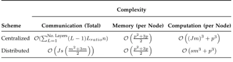
3.4 Complexity Analysis
An important aspect of a distributed algorithm is com-plexity. A centralized detection approach requires the communication of the whole data set to a central node. In addition, the classifier constructed at the central node needs to be communicated to downstream nodes. If the network is fully connected (see later), then the commu-nication complexity per node is O(mp) where p is the dimension of the data vector. The communication com-plexity of the whole network isO(J mp). If a hierarchical
Sj
Sj3
Sj1 Sj2
One-Hop Neighbours of Sj
Figure 1:Visualization of the exchange of data between nodes. NodeSjcommunicatesvikto nodesi∈Bj. Nodesi∈Bj, the one-hop neighbours of nodeSjcommunicatevki to theSj.
Algorithm 1:Distributed MVE-PCA
1 fork=1,2,. . . do
2 forall thej∈Jdo
3 ComputeAjandbjvia(13)
4 forall thej∈Jdo
5 Broadcastvkj to all neighboursi∈Bj
6 forall thej∈Jdo
7 Computeykj+1via(14)
8 Computevki+1via(15) 9 Determine subspace using(4)and(6)
10 Determine SPE for a test data instance using(7)
network is in place, then each link at the lowest level has a communication complexity of O(mp). Each link at the next level has a communication complexity of O(mp+tmp)wheretis the number of links at the lowest level into the node. If a hierarchical network of Llayers is used, then the total communication complexity is;
communication=
No. Layers X
L=1
(L−1)Lration (19)
whereLratio is the ratio of nodes in layer L.
The distributed anomaly detection algorithm requires that a node j broadcasts Aj ∈Rp×p andbj ∈Rp to its
neighbours Bj for each iteration. However,Aj is
sym-metric and therefore has a size R
p2 +p
2 . Communication
complexity is thereforeO(p2+32 p)per link per iteration. If siterations are required for convergence, the communica-tion complexity for a node isO(s(p2+32 p)). If the network is a wireless network, due to the broadcast nature of communication, the complexity isO(p2+32 p)per node per iteration. Communication complexity is dependent on the dimension of data sets and the number of iterations required to converge. However, it is independent of the number of observations on the local node, which can be very large.
MVE-PCA requires a convex optimization problem to
Table 1:Comparison of the complexities for the centralized and distributed schemes.
Complexity
Scheme Communication (Total) Memory (per Node) Computation (per Node)
Centralized O(PNo. Layers
L=1 (L−1)Lration) O p2+3p 2 O(J m)3+p3 Distributed OJ sm2+3m 2 Op2+3p 2 O sm3+p3
J=no. of nodes,n=total no. data,m=no. data instances at node,p=data dimension
s=no. iterations to converge,L=no. of layers,Lratio=ratio of nodes in Layer L
be solved on each node for each iteration. The compu-tational complexity of solving the convex optimization problem is O(m3) per node per iteration. For the cen-tralized version, all the data are available on one node and only one iteration is required. Therefore the compu-tational complexity isO((J m)3). Distributed MVE-PCA has reduced the computational complexity; as the data are distributed amongst a number of nodes, the solution of the convex optimization problem on each node is smaller as the number of data instances in the training set is smaller. The total computational complexity for the whole network is O(J m3). The algorithm requires that the convex optimization is performed multiple times as the algorithm iterates towards the solution. Therefore the total computational complexity is O(J sm3) where
s is the number of iteration to converge. Once the A
matrix has been determined, an eigen decomposition of the matrix is required in order to determine the PCs. This has a computational complexity of O(p3)for both the centralized and distributed approaches.
At each node, the storing of theAmatrix and theb vec-tor is required. The memory complexity of the distributed algorithm is O(p2+32 p), as the A matrix is symmetric. Centralized MVE-PCA also requires the storage ofAand
band therefore has the same memory complexity. Com-munication and computational complexity are detailed in Table 1 and further examined in Section 4.5.
4
E
V A L U A T I O NIn this section, evaluations on synthetic and real-world data are presented to illustrate the performance of MVE-PCA and distributed MVE-PCA. The evaluation environment is varied in order to examine the behaviour of the proposed algorithm in a broad range of settings. All algorithms are implemented in Matlab.
4.1 Evaluation Environment
The elements considered in the evaluation are network topology, network size and data sets.
4.1.1 Network Topology
Two network topologies are considered in the evalua-tion, fully connected networks and strongly connected networks. In a fully connected network, each node is connected to every other node. In a strongly connected network, there is a directed path from a vertex u to
Table 2:Real-World data sets
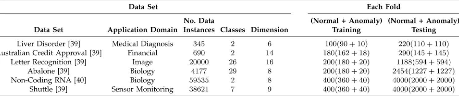
Data Set Each Fold
No. Data (Normal + Anomaly) (Normal + Anomaly)
Data Set Application Domain Instances Classes Dimension Training Testing
Liver Disorder [39] Medical Diagnosis 345 2 6 100(90 + 10) 220(110 + 110)
Australian Credit Approval [39] Financial 690 2 14 180(162 + 18) 290(145 + 145)
Letter Recognition [39] Image 20000 26 16 200(180 + 20) 1188(594 + 594)
Abalone [39] Biology 4177 29 8 200(180 + 20) 2454(1227 + 1227)
Non-Coding RNA [40] Biology 59535 2 8 400(360 + 40) 4000(2000 + 2000)
Shuttle [39] Sensor Monitoring 38621 7 9 400(360 + 40) 4000(2000 + 2000)
a vertex v, for every pair of vertices u,v. Therefore, a specific node is reachable from every other node in the network, however, the path between two nodes might be a multi-hop path via the other nodes.
Several metrics define a strongly connected network. The connections between nodes,N, are defined as edges (E), where an edge is undirected (one-way). The density of a strongly connected network,d, is defined as
d= E
N(N−1) (20) A random strongly connected network will vary in den-sity with the bounds defined as
1
L−1 6d61 (21) The lower and upper bounds of the density are achieved by the ring network and the fully connected network, respectively. The number of connections a node has also illustrates how connected a network is. Therefore the mean degree per node (MDPN) is also used.
4.1.2 Data Sets
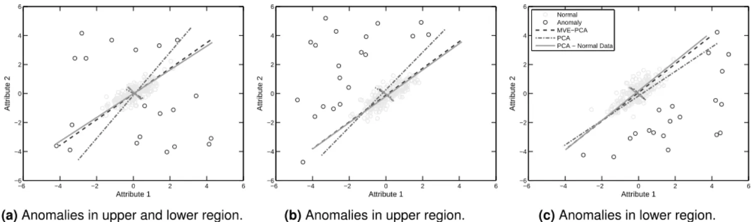
A 2-dimensional synthetic data set is used to examine the operation of the distributed anomaly detection algorithm. The normal data are formed from a Gaussian distribution N(Σ, µ)where Σ= 0.0278 0.0204 0.0204 0.0233 ! , µ= 0 0 ! (22) In order to examine the perturbation of the PCs by the anomalies, uniformly distributed anomalies are intro-duced above, below, and above and below the normal data. Anomalies form 10% of the training set. The data set is standardized by subtracting the mean and dividing by the standard deviation.
In addition to synthetic data, real-world data sets have been used to examine the performance of the distributed learning approach. In order to be employed in the evaluation of the performance of anomaly detectors, the data sets are reorganized. For the two-class data sets, the class containing more data samples is used as the normal class, while the other class is considered to be the anomaly class. For a multi-class data set, one class is considered normal, while the others are combined to form the anomaly class [41]. If the data set had a train
and validation or test set, these were concatenated. Six data sets are used from different application domains including medical diagnosis, image recognition and sen-sor measurements. The data sets exhibit a broad range of characteristics and therefore provide varied data in order to examine performance. All data sets are standardized by subtracting the mean and dividing by the standard deviation. Information regarding the real-world data sets is shown in Table 2.
The selected data sets are randomly partitioned into10 independent folds for cross-validation. For each fold, a training and a testing set are formed. For the training set, the required number of normal and anomaly data sam-ples are randomly chosen without replacement from the appropriate class of the data set. The testing set consists of an equal number of normal and anomaly samples. To form the data sets in a distributed environment, an equal number of data instances is randomly distributed across the nodes.
4.1.3 Performance Assessment
To examine performance, the area under ROC Curve (AUC) is used. The false positive rate (FPR) is the ratio of false positives to normal measurements and the true pos-itive rate (TPR) is the ratio of true pospos-itives to anomalous measurements. To compare schemes, receiver operating characteristic (ROC) curves are generated by varying the anomaly ratio used to determine the threshold distance for the residual error. Conceptually, the threshold was
varied from −∞ to +∞ and the resulting FPR and
TPR form the ROC curve. The AUC [42] is used to summarize the performance achieved. An AUC value of 1 represents 100% accuracy and an AUC value of 0.5 or lower indicates performance worse than the random assignment of labels.
In addition, the convergence of the algorithm is ex-amined. It is required that the algorithm converges to the affine transformation of the centralized version. This equates to the algorithm being able to correctly learn the scaling and rotation matrix A and the transformation vector b. To measure convergence, the relative error is used [43].
Erel=
k[A b]−[ ˜A˜b]kF
k[A b]kF
(23) where[ ˜A˜b]denote the rotation matrix and the transfor-mation vector andk · kF denotes the Frobenius norm.
−6 −4 −2 0 2 4 6 −6 −4 −2 0 2 4 6 Attribute 1 Attribute 2
(a)Anomalies in upper and lower region.
−6 −4 −2 0 2 4 6 −6 −4 −2 0 2 4 6 Attribute 1 Attribute 2
(b)Anomalies in upper region.
−6 −4 −2 0 2 4 6 −6 −4 −2 0 2 4 6 Attribute 1 Attribute 2 Normal Anomaly MVE−PCA PCA PCA − Normal Data
(c)Anomalies in lower region.
Figure 2:Comparison of the PCs derived from PCA and MVE-PCA.
In addition, the relative error is used to show how distributed MVE-PCA is able to iterate towards the objective value of the centralized version. The relative error is defined as objV al= p∗−1 J PJ j=1fj(x k) p∗ (24) The benchmark methods were chosen due to their proven performance as anomaly detectors on a wide variety of data sets. For example, in a recent performance evalu-ation by Janssens et al. [41] of five anomaly detection techniques from the fields of machine learning and knowledge discovery, the OCSVM [44] and LOF [45] outperformed other anomaly detection techniques. In another evaluation of current anomaly detection meth-ods [46],k-NN is shown to be the optimal performer for the data sets used. The Mean Centred Ellipse (MCE) [47] has also been used in a distributed environment.
4.2 MVE-PCA Evaluation
In this section, the performance of MVE-PCA is examined and compared with PCA and other benchmark anomaly detection methods. First, the 2-dimensional synthetic data set introduced in Section 4.1.2 is used to visualize the operation of MVE-PCA. Next, real-world data sets are used to examine performance. For all algorithms, parameter selection is used to determine the optimal value of the required parameters. For PCA, the subspace dimension is required. MVE-PCA requires the subspace dimension and theν parameter.
4.2.1 Visualization on a Synthetic Data Set
Fig. 2 depicts the operation of MVE-PCA on the synthetic data set. The three figures depict the axis of the two PCs determined by MVE-PCA and PCA. The PCs of PCA performed on the normal data act as a benchmark. In Fig. 2a the anomalies lie either side of the first PC, however, the PCs of PCA are still skewed by the anomalies from the actual PC obtained using only the normal data. MVE-PCA is able to determine PCs close to the actual PCs. Fig. 2b and 2c show how the anomalies that lie on one side of the normal data skew the PCs by
pulling the first PC towards them. Again, although there is skewing of the PCs of MVE-PCA, it is less pronounced than PCA. Through the use of slack variables, the effect of the anomalies on the PCs is reduced, therefore the PCs determined are closer to those derived only from the normal data.
4.2.2 Evaluation on Real-World Data Sets
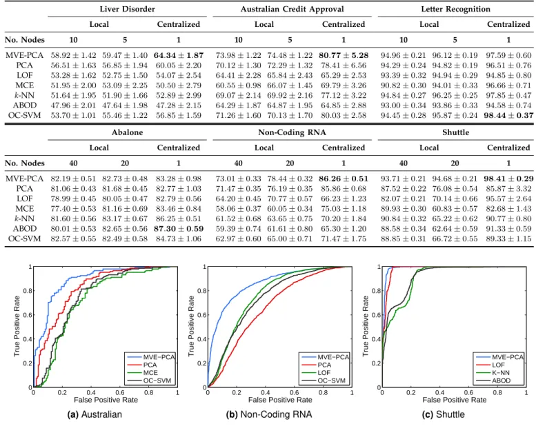
A performance evaluation to compare MVE-PCA with PCA and other state-of-the-art anomaly detection algo-rithms is performed. The results are displayed in Table 3. Both the centralized and local learning approaches are evaluated. In the centralized approach, all the data are available to one instance of the classifier. The experimen-tal results are averaged over 10 folds for each tuning, and then the highest AUC corresponding to the specific tuned parameter is reported. Therefore, the value of the specific tuned parameter varies across different data sets. For the centralized classifiers, the mean and standard deviation over the10folds are given and the bold-faced
AUC values indicate the best method for the particular data set. The ROC curves for three of the real-world data sets and the four best classifiers are illustrated in Fig. 3. In the local approach, the data are randomly dis-tributed between the nodes in the network. Each node constructs a classifier from the data available on the node. The same test data set is used across all nodes. Parameter tuning is performed on each node as for the centralized version. The mean of the local classifiers is noted and then the mean and standard deviation of the performance over the10folds are recorded in Table 3.
For most classifiers and data sets, the centralized ap-proach is significantly better than local learning. For example, with the MVE-PCA classifier and a network of 20 nodes, the Non-Coding RNA data set has an AUC of78.44±0.32whereas the centralized performance has 86.26±0.51. This trend continues across all data sets. Clearly, an increase in the number of data instances improves the classifier of the centralized version. The increased performance of the centralized classifier shows the necessity for a distributed approach where informa-tion is exchanged between nodes in order to construct a classifier that approaches that of the centralized classifier.
Table 3:UCI data sets - Comparison of centralized and local learning approaches on real-world data sets. The data are randomly distributed across the nodes. For the local learning approach the number of nodes is noted. Mean and standard deviation of 10 simulations.
Liver Disorder Australian Credit Approval Letter Recognition
Local Centralized Local Centralized Local Centralized
No. Nodes 10 5 1 10 5 1 10 5 1 MVE-PCA 58.92±1.42 59.47±1.40 64.34±1.87 73.98±1.22 74.48±1.22 80.77±5.28 94.96±0.21 96.12±0.19 97.59±0.60 PCA 56.51±1.63 56.85±1.94 60.05±2.20 70.12±1.30 72.29±1.32 78.41±6.56 94.29±0.24 94.82±0.19 96.51±0.76 LOF 53.28±1.62 52.75±1.50 54.07±2.54 64.41±2.28 65.84±2.43 65.29±2.53 93.39±0.32 94.94±0.29 94.85±0.80 MCE 51.95±2.00 53.09±2.25 50.50±2.79 60.55±0.98 66.07±1.45 69.79±3.26 90.82±0.30 94.01±0.33 96.66±0.71 k-NN 51.64±1.95 51.90±1.66 52.89±2.99 69.07±2.14 69.92±2.16 77.12±3.22 94.84±0.27 96.25±0.25 97.85±0.47 ABOD 47.96±2.01 47.64±1.98 47.28±2.15 64.29±1.87 64.87±1.95 64.85±2.88 93.00±0.34 93.86±0.33 94.58±0.74 OC-SVM 53.70±1.01 55.46±1.22 56.85±1.59 71.26±1.60 70.13±1.70 80.03±2.58 94.45±0.28 95.87±0.24 98.44±0.37
Abalone Non-Coding RNA Shuttle
Local Centralized Local Centralized Local Centralized
No. Nodes 40 20 1 40 20 1 40 20 1 MVE-PCA 82.19±0.51 82.73±0.48 83.28±0.98 73.01±0.33 78.44±0.32 86.26±0.51 93.71±0.21 94.68±0.21 98.41±0.29 PCA 81.06±0.43 81.68±0.45 82.77±1.03 71.47±0.35 76.19±0.35 85.86±0.68 87.52±0.22 76.08±0.54 85.87±3.32 LOF 78.99±0.45 80.05±0.47 82.79±0.56 64.20±0.45 70.77±0.57 66.23±1.23 82.07±0.21 70.14±0.66 95.57±2.64 MCE 77.40±0.53 81.16±0.69 83.46±0.84 58.06±0.37 60.05±0.34 75.03±1.18 89.93±0.30 60.83±0.57 82.68±1.43 k-NN 81.60±0.56 83.17±0.67 86.25±0.51 61.52±0.68 63.65±0.75 70.20±1.84 90.84±0.32 65.22±0.62 90.77±0.80 ABOD 80.01±0.53 82.65±0.56 87.30±0.59 59.39±0.74 61.61±0.80 65.30±1.20 88.58±0.34 62.64±0.59 91.33±0.59 OC-SVM 82.57±0.55 82.49±0.58 84.73±1.06 62.97±0.60 65.00±0.71 71.47±1.75 88.85±0.31 66.72±0.55 89.33±1.15 0 0.2 0.4 0.6 0.8 1 0 0.2 0.4 0.6 0.8 1
False Positive Rate
True Positive Rate MVE−PCA
PCA MCE OC−SVM (a)Australian 0 0.2 0.4 0.6 0.8 1 0 0.2 0.4 0.6 0.8 1
False Positive Rate
True Positive Rate MVE−PCA
PCA LOF OC−SVM (b)Non-Coding RNA 0 0.2 0.4 0.6 0.8 1 0 0.2 0.4 0.6 0.8 1
False Positive Rate
True Positive Rate MVE−PCA
LOF K−NN ABOD
(c)Shuttle
Figure 3:ROC curves for three of the data sets. The ROC curves of the four best performing classifiers on the data set are shown. The empirical results show that MVE-PCA is able to
outperform the other anomaly detection methods on the evaluation data sets for both the local and cen-tralized learning approach. For some data sets, such as Australian Credit Approval and Shuttle, there is a significant improvement in performance, for others such as Abalone and Non-Coding RNA the performance is similar. The other spectral method, PCA, and the kernel method OCSVM, also perform well.
In all the data sets, the spectral decomposition is able to identify a low-dimensional subspace on which the data lies, and therefore identify data samples which do not lie on this subspace (the anomalies). MVE-PCA is able to improve on the performance by reducing the influence of the anomalous data samples in the training data set, therefore improving the model of normal data and performance on the testing data set. Both the MCE and OCSVM aim to construct a model of normal data using a boundary, however the anomalies in the training
data set will influence the model constructed, therefore reducing performance on the testing data set.
The same is true for the similarity-based methods of LOF,k-NN and Angle-Based Outlier Detection (ABOD), where anomalies in the training data set will influence the classification model. An example withk-NN, if there exists a cluster ofkanomalies, an anomaly in the testing data set which has these k anomalies as the k nearest neighbours will have a low distance metric. Therefore, it is difficult to differentiate between this anomalous sample and the normal data. It is the ability of MVE-PCA to remove the influence of the anomalies in the training data set that improves performance.
Another spectral method that is robust to anomalies, Robust PCA, would not perform well in this situation. Robust PCA aims to recover a low-rank matrix, L0, and a noise component, S0 such that M = L0 +S0. An assumption is made thatS0 is sparse and therefore there are possible corruptions of individual observations in the
n-dimensional data sample. The modelling of corrupted observations is common in visual and bioinformatic data [14]. This is contrary to the anomaly detection problem here, the aim is to detect data samples where every observation of the anomalous data sample is either corrupted or generated from a different process.
4.3 Distributed Anomaly Detection - Synthetic Data Set
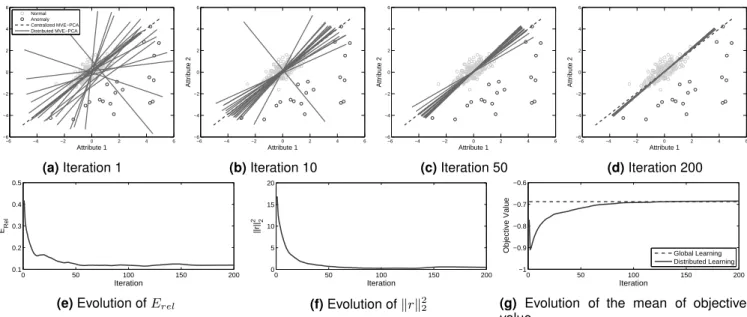
In this section, the performance of the distributed anomaly detection algorithm is examined with a syn-thetic data set. A strongly connected network of 20 nodes is considered with the data randomly distributed across all nodes. The network has a density of0.179. The number of iterations is chosen in order that convergence occurs.
Fig. 4 shows the evolution of the PCs determined by MVE-PCA and the convergence measures. In Fig. 4a the first PC derived by the nodes are shown along with the first PC derived by centralized PCA. The local PCs differ significantly across each node and differ from the centralized PC. At iteration 10, Fig. 4b, the local PCs are now closer to that of the centralized PCs. As the iterations continue, the difference between the local and centralized PCs decreases until 200 iterations have been completed, Fig. 4c, convergence has occured and there is minimal difference between the PCs on local nodes and the centralized PC.
Fig. 4e, 4f and 4g depict the evolution of the conver-gence measures. BothErel andkrkk22decrease asymptoti-cally towards zero, illustrating convergence. The objective value of the distributed approach converges to that of the centralized approach in about 100 iterations and remains constant after, further illustrating that convergence has occurred.
4.4 Distributed Anomaly Detection - Real-World Data Sets
In this section, distributed MVE-PCA is examined in environments with differing network topologies. Two types of topologies are used; a fully connected network and random strongly connected networks with differing network densities. The data sets with a training set of 200 data instances or less were distributed over five and ten nodes, and the data sets with 400 data instances were distributed over twenty and forty nodes. The real-world data sets from the centralized approach are now used in a distributed setting. 10 Monte Carlo runs are performed to reduce the effect of random elements in the simulation. As the distributed learning approach should yield a classifier that is very close to that of the centralized approach, the optimal parameters for the centralized classifier are used for the distributed classifiers. The value of ρwas chosen using parameter selection, selecting the value that allowed convergence to occur quickly and accurately. The number of iterations was chosen so that convergence occurred.
Table 4 details the results of the performance evalua-tion. The network parameters, convergence information and results are displayed. The convergence information shows that MVE-PCA is able to converge on a solution that is close to the centralized solution. The relative error for the rotation matrixAand transformation matrixbis driven to a small value during the iterations, showing that the distributed version is able to learnA andbof the centralized version. The squared norm of the primal residual,krk2
2, and the relative error of the objective func-tion,objV al, are also driven to zero, further illustrating
the convergence of the algorithm.
Although the distributed algorithm has access to the same data sets on the nodes as the local version, it is able to produce anomaly detection results that are significantly better than local learning and are similar to that of the centralized version. This is achieved by solving the distributed convex optimization problem, allowing it to iterate to the solution of the centralized version.
Distributed MVE-PCA is able to converge to perfor-mance approaching that of the centralized classifier in all cases. However, there is a difference in the accuracy amongst the data sets. Although the Australian Credit Approval and Letter Recognition data sets both use the same network sizes, the Letter Recognition data set has superior convergence, with an AUC differing from the centralized version by less than 1.0% compared to up to 3.0% for the Australian Credit Approval. Network size and topology also influence the accuracy of distributed MVE-PCA. A fully connected network (density1.0) has the best performance for all data sets. For the strongly connected networks (density<1.0), the best performance occurs with the higher density networks.
Fig. 5 illustrates the evolution of the mean of the per-formance metrics for the nodes over the iterations with different network densities. The Non-Coding RNA data set is used with 20 nodes. The AUC value,Erel,krk22and objective value are shown. Convergence occurs with all network densities, and the converged values approach or equal that of the centralized classifier. However, network density has an influence on convergence. It can be seen that the fully connected network converges faster and more accurately for the AUC Erel, krk22 and objective value. The least dense network, with a MDPN of 2.80, converges more slowly and is less accurate. An important aspect of the distributed algorithm is the time taken for convergence to be achieved. As noted by Boyd, it can take only 10s of iterations to obtain a reasonable estimate [31]. This can be seen for the Non-Coding RNA data set in Fig. 5a where an excellent AUC value is achieved in under 20 iterations.
Fig. 6 illustrates the ROC for the centralized, dis-tributed and local classifiers for three data sets. It can be seen that distributed MVE-PCA is able to obtain a similar ROC curve as centralized MVE-PCA. The local classifiers exhibit poorer performance due to the limited number of data instances in the training set.
−6 −4 −2 0 2 4 6 −6 −4 −2 0 2 4 6 Attribute 1 Attribute 2 Normal Anomaly Centralized MVE−PCA Distributed MVE−PCA (a)Iteration 1 −6 −4 −2 0 2 4 6 −6 −4 −2 0 2 4 6 Attribute 1 Attribute 2 (b)Iteration 10 −6 −4 −2 0 2 4 6 −6 −4 −2 0 2 4 6 Attribute 1 Attribute 2 (c)Iteration 50 −6 −4 −2 0 2 4 6 −6 −4 −2 0 2 4 6 Attribute 1 Attribute 2 (d)Iteration 200 0 50 100 150 200 0.1 0.2 0.3 0.4 0.5 Iteration ERel
(e)Evolution ofErel
0 50 100 150 200 0 5 10 15 20 Iteration ||r|| 2 2 (f)Evolution ofkrk2 2 0 50 100 150 200 −1 −0.9 −0.8 −0.7 −0.6 Iteration
Objective Value Global Learning Distributed Learning
(g) Evolution of the mean of objective value
Figure 4: Snapshots of the PCs derived for a synthetic training set evolving with time. The parameters areρ = 0.07and 200 iterations. A network of 20 nodes with a network density of 0.179 is used.
Table 4:UCI data sets - Comparison of centralized and distributed learning approaches on real-world data sets. The data are randomly distributed across the nodes. Mean and standard deviation of 10 simulations.
Network Convergence Performance - AUC
Nodes Density MDPN ρ Iteration Erel krk22 objV al Distributed Centralized
5 1.000 4.00 1.0 80 1.94×10⁻² 4.46×10⁻² 2.46×10⁻³ 64.34±1.97 5 0.600 2.40 1.0 80 5.56×10⁻² 5.12×10⁻² 8.28×10⁻³ 63.87±4.75 5 0.400 1.60 1.0 80 8.16×10⁻² 2.71×10⁻³ 3.45×10⁻³ 64.24±2.28 10 1.000 9.00 1.0 80 6.35×10⁻² 4.90×10⁻³ 1.74×10⁻³ 64.14±1.97 10 0.422 3.80 1.0 80 9.07×10⁻² 4.67×10⁻³ 3.96×10⁻³ 63.87±2.02 Liver Disorder 10 0.311 2.80 1.0 80 1.15×10⁻¹ 3.34×10⁻² 7.44×10⁻³ 63.56±2.14 64.34±1.87 5 1.00 4.00 0.1 50 1.72×10⁻² 8.28×10⁻³ 5.01×10⁻⁵ 80.76±5.29 5 0.600 2.40 0.1 50 8.45×10⁻² 1.16×10⁻³ 1.32×10⁻³ 79.00±8.26 5 0.400 1.60 0.1 50 3.91×10⁻¹ 9.96×10⁻³ 1.70×10⁻² 77.97±4.59 10 1.00 9.00 0.1 50 1.58×10⁻² 1.98×10⁻² 1.00×10⁻⁴ 80.76±5.25 10 0.422 3.80 0.1 50 3.40×10⁻² 3.47×10⁻² 4.77×10⁻³ 80.13±6.23 Australian Credit Approval
10 0.311 2.80 0.1 50 2.78×10⁻¹ 2.04×10⁻¹ 5.54×10⁻³ 81.51±4.99 80.77±5.28 5 1.00 4.00 0.1 25 9.73×10⁻² 1.87×10⁻¹ 5.83×10⁻³ 97.46±0.58 5 0.600 2.40 0.1 25 1.06×10⁻¹ 1.82×10⁻¹ 5.56×10⁻³ 97.39±0.55 5 0.400 1.60 0.1 25 1.43×10⁻¹ 1.88×10⁻¹ 9.86×10⁻² 97.10±0.73 10 1.00 9.00 0.5 50 2.50×10⁻² 1.76×10⁻¹ 1.30×10⁻³ 97.56±0.61 10 0.422 3.80 0.5 50 3.66×10⁻² 1.97×10⁻¹ 5.04×10⁻³ 97.48±0.70 Letter Recognition 10 0.311 2.80 0.5 50 6.07×10⁻² 2.06×10⁻¹ 6.03×10⁻³ 97.32±0.70 97.56±0.48 20 1.00 19.00 0.1 100 3.14×10⁻³ 1.02×10⁻¹ 8.31×10⁻⁴ 83.23±1.04 20 0.211 4.00 0.1 100 2.06×10⁻² 1.23×10⁻¹ 2.10×10⁻³ 83.18±1.16 20 0.147 2.80 0.1 100 2.19×10⁻² 1.43×10⁻¹ 3.38×10⁻³ 83.00±1.27 40 1.00 39.00 0.1 150 3.18×10⁻³ 1.93×10⁻¹ 1.09×10⁻³ 83.23±1.04 40 0.209 8.15 0.1 150 1.81×10⁻² 2.21×10⁻¹ 1.55×10⁻³ 83.09±1.14 Abalone 40 0.159 6.20 0.1 150 1.79×10⁻² 2.15×10⁻¹ 2.48×10⁻³ 83.10±1.17 83.28±0.98 20 1.00 19.00 0.1 50 3.76×10⁻³ 9.57×10⁻² 9.10×10⁻⁵ 86.25±0.52 20 0.211 4.00 0.1 50 6.56×10⁻² 7.04×101 7.65×10⁻³ 86.10±0.46 20 0.147 2.80 0.1 50 3.80×10⁻² 6.23×10⁻¹ 1.22×10⁻² 86.17±0.83 40 1.00 39.00 0.05 100 3.01×10⁻³ 1.81×10⁻¹ 1.96×10⁻⁴ 86.25±0.50 40 0.209 8.15 0.05 100 1.99×10⁻² 4.84×10⁻¹ 1.42×10⁻³ 86.15±0.56 Non-Coding RNA 40 0.159 6.20 0.05 100 2.61×10⁻² 5.18×10⁻¹ 3.03×10⁻³ 86.33±0.58 86.26±0.51 20 1.00 19.00 0.1 50 6.18×10⁻⁴ 1.68×10⁻² 3.64×10⁻⁶ 98.41±0.29 20 0.211 4.00 0.1 50 2.14×10⁻² 4.67×10⁻² 1.86×10⁻³ 98.08±0.89 20 0.147 2.80 0.1 50 1.91×10⁻² 9.24×10⁻² 1.45×10⁻³ 98.35±0.41 40 1.00 39.00 0.1 100 5.20×10⁻⁴ 1.59×10⁻² 3.10×10⁻⁶ 98.41±0.29 40 0.209 8.15 0.1 100 1.02×10⁻² 2.04×10⁻² 2.14×10⁻⁴ 98.42±0.29 Shuttle 40 0.159 6.20 0.1 100 1.33×10⁻² 3.23×10⁻² 2.70×10⁻⁴ 98.40±0.31 98.41±0.29
0 5 10 15 20 25 30 35 40 45 50 0.5 0.6 0.7 0.8 0.9 1 Iteration AUC Global Learning MDPN − 2.80 MDPN − 4.00 MDPN − 19.00
(a)Evolution of AUC
0 5 10 15 20 25 30 35 40 45 50 0 0.2 0.4 0.6 0.8 Iteration ERel MDPN − 2.80 MDPN − 4.00 MDPN − 19.00 (b)Evolution ofErel 0 5 10 15 20 25 30 35 40 45 50 0 2 4 6 8 10 Iteration ||r|| 2 2 MDPN − 2.80 MDPN − 4.00 MDPN − 19.00 (c)Evolution ofkrk2 2 0 5 10 15 20 25 30 35 40 45 50 −0.65 −0.6 −0.55 −0.5 −0.45 −0.4 −0.35 −0.3 Iteration Objective Value Global Learning MDPN − 2.80 MDPN − 4.00 MDPN − 19.00
(d)Evolution of the objective value Figure 5:The Non-Coding RNA data set with a network of 20 nodes and different network densities.
0 0.2 0.4 0.6 0.8 1 0 0.2 0.4 0.6 0.8 1
False Positive Rate
True Positive Rate Centralized
Distributed − Node 1 Local − Node 1 Local − Node 2 (a)Australian 0 0.2 0.4 0.6 0.8 1 0 0.2 0.4 0.6 0.8 1
False Positive Rate
True Positive Rate Centralized
Distributed − Node 1 Local − Node 1 Local − Node 2 (b)Non-Coding RNA 0 0.2 0.4 0.6 0.8 1 0 0.2 0.4 0.6 0.8 1
False Postive Rate
True Postive Rate Centralized
Distributed − Node 1 Local − Node 1 Local − Node 2
(c)Shuttle Figure 6:ROC curves for three of the data sets. Centralized and distributed and local learning.
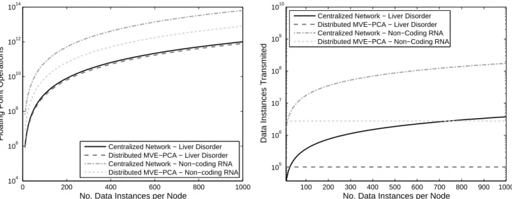
4.5 Complexity Analysis
This section examines the computational and commu-nication complexity of the centralized and distributed learning approach for the evaluation networks. For the centralized approach, a hierarchical network is assumed. A three layer multi-level hierarchical topology is used with leaf nodes, intermediate parent nodes and a gateway node [3], [4]. It is assumed that 3/4 of the nodes are in layer 3, with the remaining nodes in layer two which transmit to a central node. The classifier is constructed on the central node. The computational complexity of the centralized and distributed approaches are displayed in Fig. 7a. Computational complexity for the distributed learning approach is lower than that of the centralized approach. Although the distributed approach requires the solution of multiple convex optimization problems at node level to iterate towards the solution, it has a
much smaller data set on each node. As the solution of the convex optimization problems is dependent on the number of data instances in the training set, this reduces computational complexity. This is the case for the Liver Disorder data set with 10 nodes and the Non-Coding RNA data set with 40 nodes.
Communication complexity is displayed in Fig. 7b. The communication cost for the centralized approach is calculated using (19). For the centralized approach, com-munication complexity increases rapidly as the number of data instances on individual data nodes increases for both the Liver Disorder and Non-Coding RNA data sets. Distributed MVE-PCA has a constant communication complexity regardless of the number of data instances on a node. Communication complexity depends on the size of the matrix A and the vectorb. These summary statistics are transmitted by a node to neighbouring
0 200 400 600 800 1000 104 106 108 1010 1012 1014
No. Data Instances per Node
Floating Point Operations
Centralized Network − Liver Disorder Distributed MVE−PCA − Liver Disorder Centralized Network − Non−coding RNA Distributed MVE−PCA − Non−coding RNA
(a)Computational complexity of centralized MVE-PCA and dis-tributed MVE-PCA. 100 200 300 400 500 600 700 800 900 1000 105 106 107 108 109 1010
No. Data Instances per Node
Data Instances Transmited
Centralized Network − Liver Disorder Distributed MVE−PCA − Liver Disorder Centralized Network − Non−Coding RNA Distributed MVE−PCA − Non−Coding RNA
(b)Communication complexity for centralized learning in a hier-archical network and distributed MVE-PCA.
Figure 7:Complexity analysis with the Liver Disorder and Non-Coding RNA data set. nodes, and using distributed MVE-PCA the algorithm is
able to iterate towards the centralized classifier without the transmission of the data set to a central node. A drawback of the approach is the requirement to transmit the matrixAand the vectorbeach round as the algorithm iterates towards the final solution. However, Fig. 7b shows that the communication complexity is significantly lower than that of the centralized version except when there is a small number of data instances on an individual node.
5
C
O N C L U S I O NA robust PCA-based anomaly detection algorithm that operates in a distributed environment was proposed. Minimum volume elliptical PCA is able to determine the PCs more robustly in the presence of anomalies by constructing a soft-margin minimum volume ellipse around the data that reduces the influences of anomalies in the training set. Evaluations on real-world data sets show that the performance of minimum volume PCA exceeds that of PCA and other state-of-the-art anomaly detection techniques.
Local and centralized approaches to anomaly detection were examined. It was shown that a local approach can lead to poor performance compared to the centralized approach. A solution to this issue is distributed learning which can provide performance that approaches that of the centralized classifier. The proposed anomaly de-tection technique was reformulated using a distributed convex optimization problem which splits the problem across a number of nodes. Communication between nodes is limited to the exchange of small matrices be-tween neighbouring nodes where no specific network infrastructure is assumed. Evaluation of the distributed minimum volume PCA on synthetic and real-world data sets shows that the distributed algorithm is able to approach the performance of the centralized version.
R
E F E R E N C E S[1] V. Barnett and T. Lewis,Outliers in Statistical Data. New York: Wiley, Apr. 1994.
[2] V. Chandola, A. Banerjee, and V. Kumar, “Anomaly detection: A survey,”ACM Computing Surveys, vol. 41, no. 3, pp. 15:1–15:58, Jul. 2009.
[3] S. Rajasegarar, C. Leckie, and M. Palaniswami, “Hyperspherical cluster based distributed anomaly detection in wireless sensor networks,”J. of Parallel and Distributed Computing, vol. 74, no. 1, pp. 1833–1847, 2014.
[4] S. Rajasegarar, A. Gluhak, M. Ali Imran, M. Nati, M. Moshtaghi, C. Leckie, and M. Palaniswami, “Ellipsoidal neighbourhood outlier factor for distributed anomaly detection in resource constrained networks,”Pattern Recognit., pp. 1–13, Apr. 2014.
[5] P. Rousseeuw, “Multivariate estimation with high breakdown point,” in 4th Pannonian Symp. on Mathematical Statistics and Probability, Bad Tatzmannsdorf, Austria, Sep. 1983.
[6] D. Mosk-Aoyama, T. Roughgarden, and D. Shah, “Fully distributed algorithms for convex optimization problems,”J. on Optimization, vol. 20, no. 6, pp. 3260–3279, 2010.
[7] F. Angiulli, S. Basta, S. Lodi, and C. Sartori, “Distributed strategies for mining outliers in large data sets,”IEEE Trans. Knowl. Data Eng., vol. 25, no. 7, pp. 1520–1532, 2013.
[8] M. Xie, J. Hu, S. Han, and H.-H. Chen, “Scalable hypergrid k-NN-based online anomaly detection in wireless sensor networks,”
IEEE Trans. Parallel Distrib. Syst., vol. 24, no. 8, pp. 1661–1670, 2013. [9] H. Hotelling, “Analysis of a complex of statistical variables into
principal components,”J. of educational psychology, vol. 24, 1933. [10] V. Chatzigiannakis and S. Papavassiliou, “Diagnosing anomalies
and identifying faulty nodes in sensor networks,”IEEE Sensors J., vol. 7, no. 5, pp. 637–645, 2007.
[11] A. Lakhina, M. Crovella, and C. Diot, “Diagnosing network-wide traffic anomalies,”ACM SIGCOMM Computer Communication Review, pp. 219–230, 2004.
[12] M. A. Livani and M. Abadi, “Distributed PCA-based anomaly detection in wireless sensor networks,” in5th Int. Conf. for Inter-net Technology and Secured Transactions (ICITST), London, United Kingdom, Nov. 2010, pp. 1–8.
[13] L. Huang, X. Nguyen, M. Garofalakis, M. I. Jordan, A. Joseph, and N. Taft, “In-network PCA and anomaly detection,” inAdvances in Neural Information Processing Systems, Vancouver, B.C, Dec. 2006, pp. 617–624.
[14] J. Wright, A. Ganesh, S. Rao, Y. Peng, and Y. Ma, “Robust principal component analysis: Exact recovery of corrupted low-rank matri-ces via convex optimization,” in Advances in Neural Information Processing Systems, Vancouver, BC, Dec. 2009, pp. 2080–2088.