Refining value-at-risk estimates using a Bayesian Markov-switching GJR-GARCH copula-EVT model

Refining value-at-risk estimates using a

Bayesian Markov-switching GJR-GARCH

copula-EVT model

Marius Galabe Sampid, Haslifah M. Hasim*, Hongsheng Dai

Department of Mathematical Sciences, University of Essex, Colchester, United Kingdom

*[email protected]

Abstract

In this paper, we propose a model for forecasting Value-at-Risk (VaR) using a Bayesian Markov-switching GJR-GARCH(1,1) model with skewed Student’s-t innovation, copula functions and extreme value theory. A Bayesian Markov-switching GJR-GARCH(1,1) model that identifies non-constant volatility over time and allows the GARCH parameters to vary over time following a Markov process, is combined with copula functions and EVT to formu-late the Bayesian Markov-switching GJR-GARCH(1,1) copula-EVT VaR model, which is then used to forecast the level of risk on financial asset returns. We further propose a new method for threshold selection in EVT analysis, which we term the hybrid method. Empirical and back-testing results show that the proposed VaR models capture VaR reasonably well in periods of calm and in periods of crisis.

Introduction

In recent decades, Value-at-Risk (VaR) has become a key tool for measuring market risk; it provides risk managers with a quantitative measure of the downside risk of a firm or invest-ment portfolio during a given time frame. VaR attempts to summarise the total risk in a port-folio of asset or exposures to risk factors in a single number over a target horizon.

There are several methods to estimate VaR; the most commonly used by financial institu-tions are the variance-covariance, historical simulation and Monte Carlo simulation methods (see [1–3] and the references therein). Historical simulation relies on actual data and is based on the assumption that history will repeat itself; the VaR is estimated by running hypothetical portfolios from historical data [4]. The variance-covariance and Monte Carlo simulation meth-ods assume that asset returns are independent and identically distributed, a major weakness in these VaR models.

Traditional VaR models assume asset returns in financial markets to be normally distrib-uted; thus, changes in asset prices are independent of each other and exhibit constant vola-tility over time. This is not the case in real life i.e., financial asset returns are leptokurtic and a1111111111 a1111111111 a1111111111 a1111111111 a1111111111 OPEN ACCESS

Citation: Sampid MG, Hasim HM, Dai H (2018)

Refining value-at-risk estimates using a Bayesian Markov-switching GJR-GARCH copula-EVT model. PLoS ONE 13(6): e0198753.https://doi.org/ 10.1371/journal.pone.0198753

Editor: Cathy W.S. Chen, Feng Chia University,

TAIWAN

Received: September 8, 2017 Accepted: May 24, 2018 Published: June 22, 2018

Copyright:©2018 Sampid et al. This is an open access article distributed under the terms of the

Creative Commons Attribution License, which permits unrestricted use, distribution, and reproduction in any medium, provided the original author and source are credited.

Data Availability Statement: The data employed in

this analysis consist of 2870 daily observations of stock prices from 31 December 2004 to 31 December 2015. The stocks are actively traded on the London Stock Exchange and belong to the banking sector; they are: HSBC Holdings, Lloyds Banking Group, Barclays Plc., Royal Bank of Scotland Group, and Standard Chartered Plc. We refer to these banks as Bank 1, Bank 2, Bank 3, Bank 4, and Bank 5 in the manuscript. All relevant data are available from datastream; a database for financial and economic research data from Thomas Reuters, which is a third-party database, and not

heavy tailed with non-constant volatility [5,6]. The normality assumption leads to inaccu-rate estimates in the tails of the distribution and hence of the probability of extreme events, which leads to underestimation of the likelihood of extreme tail losses. This is because the normal distribution has light tails, and VaR attempts to capture the behaviour of the portfo-lio return in the left tail. A model based on the normal distribution underestimates the fre-quency of outliers and hence the true VaR [2]. Additionally, the normality assumption implies volatility is constant over time, and recent price changes, which are based on cur-rent market information, will be assigned weights in equal proportion to older ones. If the dependence characteristics of the extreme realisations differ from all others in the sample, the consequences might be dire [7].

Non-normality for univariate models is associated with the dependence (i.e., correlation) structure between the asset returns. For multivariate models, non-normality is associated with the joint probability of the univariate models’ marginal probabilities, i.e., the joint probability of large market movements, known astail dependence. Because of the complexity of multivari-ate distributions, the VaR estimation of a portfolio of assets can be quite difficult. To avoid the normality assumption, extreme value theory (EVT) is often used to model the tail behaviour of asset returns. However, EVT also assumes extreme events to be independent and identically distributed, which might not hold in periods of severe crisis [8]. [9] suggests applying EVT to the noise variables of the return series, which are normally distributed, to obtain theqth quan-tile used to estimate conditional, robust VaR estimates. By doing so, the problem of volatility clustering and other related effects, such as excess kurtosis, is accounted for. This approach was further investigated by [4]; they combined a GARCH(1,1) model as the underlying volatil-ity model with EVT to estimate the VaR of the Tunisian stock market index and showed that the GARCH-EVT-based VaR approach appears to be more effective and realistic than tradi-tional VaR estimation methods.

A study by [10] have shown that volatility predictions following econometric models that ignore regime changes and time varying parameters have several drawbacks. For example, they may fail to capture the dynamics of fluctuations in the time series data. Ignoring regime changes and time varying parameters in high-volatility periods causes significant upwards bias in estimating the GARCH parameters, which impairs volatility forecasts [11]. The Markov-switching GARCH model, first developed by [12] and later improved by [11,13], helps address the issues since it allows the parameters of GARCH models to vary over time according to a latent discrete Markov process, which leads to volatility forecasts that can rapidly adapt to vari-ations [14].

The problem of dependence can also be improved with the help of copula theory, which enables the construction of flexible multivariate distributions with different margins and dependence structures. This allows the joint distribution of the portfolio to be free from assumptions of normality and linear correlation. [15,16] have demonstrated that VaR esti-mates obtained by combining GARCH models, EVT and copula functions are more accurate than those obtained using traditional VaR estimation methods or methods that combined cop-ulas with conventionally employed empirical distributions.

In this paper, we combine the Bayesian Markov-switching GJR-GARCH(1,1) model with skewed Student’s-tdistribution, copula functions and the peaks over threshold (POT) method of EVT to estimate VaR in selected banks in the United Kingdom (UK) using actively traded stocks on the London Stock Exchange.

owned by the authors (http://financial. thomasonreuters.com/en/products/tools- applications/trading-investment-tools/datastrean-macroeconomic-analysis.html). Other researchers will be able to access these data in the same manner as the authors.

Funding: The author(s) received no specific

funding for this work.

Competing interests: The authors have declared

Methodology

Markov-switching GJR-GARCH model

Letrtrepresent a time series, then a general Markov-switching GARCH specification can be represented as rtjðDt¼k;Ot 1Þ Dð0;hk;t;YkÞ; ð1Þ rt¼t h 1 2 D_t;t ; ð2Þ

whereΔtis a Markov chain (a stochastic variable) defined on the parameter spaceS= {1,. . .,

K} that symbolises the model,D(0,hk,t,Θk) is a continuous distribution with zero mean and conditional variancehk,t,tis the distribution of the noise variables, which assumes a skewed Student’s-tdistribution,Ot−1is the information set observed up to timet− 1, andΘkis a vector of the shape parameters.

We define aK×Ktransition probability matrix P, with distinctive elements

p_ij¼P½D_t¼jjD_t 1¼iŠ; 8i;j2 f1;. . .;Kg; 0<pij<1; S K

j¼1pij¼1; ð3Þ wherepijis the probability of transition from stateΔt−1=ito stateΔt=j.krepresents each regime in the Markov chain. The conditional variance,hk,t, fork= 1,. . .Kare assumed to fol-lowK-separateGARCH-type processes which evolve in parallel [11,14]. The Markov switch-ing GARCH models use a stochastic process to define the unknown states [17].

The reliability of a good VaR model depends on the type of volatility model which it incor-porates. As discussed above, most financial asset returns are not independently and identically distributed; they exhibit fat tails, leverage effects, and volatility is not constant over time. Vola-tility reacts differently with large negative returns as compared to positive returns reflecting leverage effects [2]. GARCH models often fail to capture these movements. A good volatility estimator must be able to capture the true behaviour of risk factor returns, it should be easy to implement for a wide range of risk factors, and finally, it should be possible to extent the approach to portfolios with a number of different risk factors [3]. It is well known that tradi-tional GARCH models cannot capture the asymmetric response of volatility. Several other extensions of GARCH models have since been developed as possible solutions to these draw-backs. The most common of these are the exponential generalised ARCH (EGARCH) model [18], the threshold GARCH (TGARCH) model [19], and the GJR-GARCH model [20]. The only significant, albeit minor, difference between TGARCH and GJR-GARCH models is that TGARCH uses standard deviation instead of variance in its specifications [21]. We employ the Markov-switching GARCH model of [11] to capture the differences in the variance dynamics of high and low volatility periods [14], and use the GJR-GARCH(1,1) model to capture the asymmetry response in the conditional volatility process, hence the Markov-switching GJR-GARCH(1,1) model (MS-GJR-GARCH(1,1)).

The conditional variance of a MS-GJR-GARCH model is defined as

hk;t¼a0;kþ ða1;kþa2;kIfrt 1<0gÞr

2

t 1þbkhk;t 1; k¼1;. . .K; ð4Þ

whereIfgis an indicator function introduced to capture the leverage effect such that

I_{t 1} ¼

(

1; if rt 1 <0;

0; if rt 1 0:

α2,kcontrols the degree of asymmetry in the conditional volatility to the past shock in regimek [14]. Thus,α2,k>0 indicates the presence of leverage effect which implies previous negative returns have higher influence on the volatility. The constraintsα0,k>0,α1,k+α2,k0 andβk

0 ensures a positive variance while covariance stationary is achieved by ensuring that a1;kþa2;kE½

2

k;tIf_k;t<0gŠ þbk <1; ð6Þ

whereIf:g ¼1if the condition holds and 0 otherwise. Note thatE½

2

k;tIf_k;t<0gŠ ¼

1

2whenkis

symmetrically distributed.

For the conditional distribution ofrtin each regime of the Markov chain, we employ a skew and fat tail error probability distribution; the skewed Student’s-tdistribution. We use the skewed Student’s-tdistribution because it is able to account for the excess kurtosis in the con-ditional distribution that is common with financial time series processes [22]. Moreover, recent studies by [23,24] have shown that skewed Student’s-terrors distribution is a good choice, when compared to a range of existing alternatives. The probability density function (PDF) of a Student’s-tdistribution is defined as

fsð;nÞ ¼ G nþ1 2 ffiffiffiffiffiffiffiffiffiffiffiffiffiffiffiffiffiffiffiffiffiffiffiffiffiffiffi ðn 2ÞpG n 2 q 1þ 2 n 2 nþ1 2 ; 2R; _ð7Þ

where the constraint on the degrees of freedom parameterν>2 is imposed to guarantee that the second order moment exist, andΓ() is the Gamma function. Skewness is introduced by an additional parameterγk>0 as defined in [25]; that is

pð_kjv;g_kÞ ¼ 2 g_kþ 1 g_k fs _k g_k I½0;1ÞðkÞ þfsðgkkÞIð 1;0ÞðkÞ : ð8Þ

Whenγk6¼1, the posterior distribution,p(k|v,γk) loses symmetry (see [14,25,26] for more details on skewed Student’s-tprobability distribution).

We use Bayesian statistics to estimate the posterior distribution of the variance equation because the Bayesian estimation method provides reliable results even for finite samples. Moreover, it is usually straightforward when using the Bayesian estimation method, to obtain the posterior distribution of any non-linear function of the model parameter. By comparison, when using the classical maximum likelihood method, it is not easy to perform inferences on non-linear functions of the model parameters, while the convergence rate is slow and presents limitations when the residuals are heavy tailed. The constraints on the GARCH parameters to guarantee a positive variance can be incorporated via priors whereas the classical maximum likelihood method may impede some optimisation procedures [27,28].

We define a vector of the risk factor returns as r = (r1,. . .,rT)0,θk= (α0,k,α1,k,α2,k,βk, P)0, and a vector of the model parameters asΛ= (θ1,Θ1,. . .,θK,ΘK);ΘK= (νK,γK). Then, from Bayes theorem and prior distribution of the model parametersp(Λ), we have

p_ij¼ Pr½D_t¼jjD_t 1 ¼iŠ ¼

fðrtjDt¼j;Ot 1;LÞPrðDt¼jjOt 1Þ Sk_i¼1fðrtjDt¼i;Ot 1;LÞPrðD¼ijOt 1Þ

; ð9Þ

wheref(rt|Δt=j,Ot−1;Λ) is the conditional probability density ofrtat timetrestrictive onOt−1 and regimej. Therefore we have

fðrtjL;Ot 1Þ ¼ Xk i¼1 Xk j¼1 Pr½D_t¼jjD_t 1¼iŠfDðrtjDt¼j;Ot 1;LÞ ð10Þ

and a likelihood function

LðLjrÞ ¼Y

T

t¼1

fðrtjL;Ot 1Þ: ð11Þ

The Metropolis Hasting (MH) algorithm of Markov Chain Monte Carlo (MCMC) is then employed to estimate the parameter values of the posterior distribution. As discussed in [22], because of the recursive nature of the variance equation, the prior densityp(Λ) and posterior densityp(r|Λ) do not belong to the same distributional family and, consequently, cannot be

expressed in close form. The MH algorithm allows draws to be generated from any density and whose normalising constant is unknown.

In the MH algorithm,Λis a random variable with Markov chains generated as (Λ[0] ),. . ., (Λ[j]

),. . .in a parameter space. As the number of realised chains reaches infinity,p(r|Λ) tends

to a normalised probability distribution with a random variable (Λ[j]

) [29]. The chain con-verges to its stationary distribution and the optimal mean values of the posterior distribution parameters are realised. [22] summarises the MH algorithm as follows: (i) Initialise the itera-tion counter toj= 1 and set the initial valueΛ[0]. (ii) Move the chain to a new valueΛ? gener-ated from a proposal densityq(|Λ[j−1]_{). (iii) Evaluate the acceptance probability of the move} fromΛ[j−1]toΛ[?]given by min pðL ? jrÞ pðL½j 1ŠjrÞ qðL½j 1ŠjL?Þ qðL?jL½j 1ŠÞ;1 ( ) :

If the move is accepted, setΛ[j]=Λ?; if not, setΛ[j]=Λ[j−1](i.e., the chain does not move). If chosen from a symmetric proposal density, i.e.,q(Λ[j]_|Λ?

) =q(Λ?_|Λ[j]

), then the acceptance probability reduces to min pðL ? jrÞ pðL½jŠjrÞ;1 ( ) :

(iv) Finally, change the counter fromjtoj+ 1 and go back to step (ii) until convergence is reached. More details on MH algorithms can be found in [30–33].

Copula theory

Copula theory enables the construction of a flexible multivariate distribution with varying margins and dependence structures; it is free from assumptions of normality or linear correla-tion. In addition, copulas can easily capture the tail dependence of asset returns, i.e., the joint probability of large market movements.

Copula theory was first developed by [34] to describe the dependence structure between random variables. It was later introduced to the finance literature by [35,36]. Consequently, [37] introduced the application of copula theory to financial asset returns, and [38] expanded the framework of copula theory with respect to the time-varying nature of financial depen-dence schemes. Copula theory has also been used in risk management to measure the VaR of portfolios, including both unconditional [39–41] and conditional distributions [42–44].

In multivariate settings, we use the following version of Sklar’s theorem as given by [41] for the purpose of VaR estimation:

Sklar’s theorem: Consider ann-dimensional joint distributional functionF(x), with uni-form marginsF1(x1),. . .,Fn(xn);x= (x1,. . .,xn), with−1 xi 1, then there exists a copula

C: [0, 1]n![0, 1] such that

Fðx1;. . .;xnÞ ¼CðF1ðx1Þ; ;FnðxnÞÞ; ð12Þ determined under absolute continuous margins as

Cðu1;. . .;unÞ ¼FðF

1

1 ðu1Þ; ;F 1

n ðunÞÞ; ð13Þ otherwise,Cis uniquely determined on the rangeR(F1)×. . .×R(Fn). Equally, ifCis a copula andF1,. . .,Fnare univariate distribution functions, thenEq (12)is a joint distribution func-tion with marginsF1,. . .,Fn[45].

The copulaC(u1,. . .,un) has densityc(u1,. . .,un) associated to it and defined as

cðu1;. . .;unÞ ¼

@_nCðu1;. . .;unÞ

@u1;. . .; @un

ð14Þ

and is related to the density functionFfor continuous random variables denoted asf, by the canonical copula representation [16]

fðx1;. . .;xnÞ ¼cðF1ðx1Þ;. . .;FnðxnÞÞ Yn

i¼1

fiðxiÞ; ð15Þ

wherefiare the marginal densities that can be different from each other [41,43,45,46]. [16,47] discuss two commonly used families of copulas in financial applications: the ellipti-cal and the Archimedean copulas.

Elliptical copulas are derived from the elliptical distribution by applying Sklar’s theorem. The most common are the Gaussian and the Student’s-tcopulas, which are symmetric. Their dependence structure is determined by a standardised correlation or dispersion matrix because of the invariant property of copulas. Consider a symmetric positive definite matrixρ

withdiag(ρ) = (1, 1,. . ., 1)T; we can represent the multivariate Gaussian copula (MGC) as

CG_a r ¼FrðF 1 ðu1Þ;. . .;F 1 ðunÞÞ; ð16Þ

whereFρis the standardised multivariate normal distribution andFr1is the inverse standard

univariate normal distribution function ofuwith correlation matrixρ. If the margins are nor-mal, then the Gaussian copula will generate the standard Gaussian joint distribution function with density function

cG_a r ðu1;u2;. . .;unÞ ¼ 1 jrj 1 2 exp 1 2B 0 ðr 1 _IÞB ; _ð17Þ whereB¼ ðF 1ðu1Þ;. . .;F 1

ðu_nÞÞ0andIis the identity matrix.

On the other hand, the multivariate Student’s-tcopula (MTC) has the form

Tr;vðu1;. . .;unÞ ¼tr;vðt

1

v ðu1Þ;. . .;t 1

v ðunÞÞ ð18Þ with density function

cr;vðu1;. . .;unÞ ¼ jrj 1 2G vþn 2 G v 2 G v 2 G vþ1 2 !n 1þ 1 vB 0 r 1_B vþ2n Q_n j¼1 1þ B2 j v vþ1 2 ; _ð19Þ

wheretρ,vis the standardised Student’s-tdistribution with correlation matrixρandvdegrees of freedom.

Archimedean copulas are useful in risk management analysis because they capture asym-metric tail dependencies between financial asset returns. The most common are the Gumbel [48], Clayton [49] and Frank [50] copulas [51]. These copulas are built via a generator as

Cðu1;. . .;unÞ ¼φ

1_ðφðu

1Þ þ. . .þφðunÞÞ ð20Þ with density function

cðu1;. . .;unÞ ¼φ 1 ðφðu1Þ þ. . .þφðunÞÞ Yn i¼1 φ0ðuiÞ; ð21Þ

whereφis the copula generator andφ−1is completely monotonic on [0,1]. That is,φmust be infinitely differentiable with derivatives of ascending order and alternative sign such that

φ−1(0) = 1 and limx!+1φ(x) = 0 [47]. Thus,φ0(u)<0 (i.e.,φis strictly decreasing) andφ00(u)

>0 (i.e.,φis strictly convex).

The Gumbel copula captures upper tail dependence, is limited to positive dependence, and has generator functionφ(u) = (−ln(u))αand generator inverseφ 1_{ðxÞ ¼ exp x}1

a

. This will generate a Gumbeln-copula represented by

Cðu1;. . .;unÞ ¼ exp Xn i¼1 ð lnuiÞ a " #1 a 8 > > < > > : 9 > > = > > ; a>1: ð22Þ

The generator function for the Clayton copula is given byφ(u) =u−α− 1 and generator inverseφ 1_{ðxÞ ¼ ðxþ1Þ} 1a_{, which yields a Claytonn-copula represented by}

Cðu1;. . .;unÞ ¼ Xn i¼1 u a i nþ1 " # 1 a a>0: ð23Þ

Frank copula has generator functionφðuÞ ¼ ln exp_expð_ða_au_ÞÞ₁1

and generator inverse

φ 1_{ðxÞ ¼} 1

alnð1þe

x_ðe a _{1ÞÞ, which will result in a Frankn-copula represented by}

Cðu1;. . .;unÞ ¼ 1 aln 1þ Q_n i¼1ðe au_{i 1Þ} ðe a _1Þn 1 ( ) a>0: ð24Þ

We follow [52] and employ Gaussian, Student’s-t, Gumbel, Frank and Clayton copulas in this study.

Modelling dependence

The traditional way to measure the relationship between markets and risk factors is to look at their linear correlations, which depend both on the marginal and joint distributions of the risk factors. If there is a non-linear relationship (i.e., in the case of non-normality) the results might be misleading [47]. In this situation, non-parametric invariant measures that are not dependent on marginal probability distributions such as Kendall’sτor Spearman’sρare more appropriate. Copulas measure a form of dependence between pairs of risk factors (i.e., asset returns) known as concordance using these invariant measures.

Two observations (xi,yi) and (xj,yj) from a vector (X,Y) of continuous random variables are concordant if (xi−xj)(yi−yj)>0 and discordant if (xi−xj)(yi−yj)<0. Large values ofX

are paired with large values ofYand small values ofXare paired with small values ofYas the proportion of concordant pairs in the sample increases. On the other hand, the proportion of concordant pairs decreases as large values ofXare paired with small values ofYand small val-ues ofXare paired with large values ofY[53].

Considernpaired continuous observations (xi,yi) ranked from smallest to largest, with the smallest ranked 1, the second smallest ranked 2, and so on. Then, Kendall’sτis defined as the sum of the number of concordant pairs minus the sum of the number of discordant pairs divided by the total number of pairs, i.e., the probability of concordance minus the probability of discordance:

t_X;Y ¼ Pr½ðxi xjÞðyi yjÞ>0Š Pr½ðxi xjÞðyi yjÞ<0Š ¼

C D

CþD; ð25Þ

whereCis the number of concordant pairs below a particular rank that are larger in value than that particular rank, andDis the number of discordant pairs below a particular rank that are smaller in value than that particular rank.

Spearman’sρ, on the other hand, is defined as the probability of concordance minus the probability of discordance of the pair of vectors (x1,y1) and (x2,y3) with the same margins. That is,

r_X;Y ¼3ðPr½ðx1 x2Þðy1 y3Þ>0Š Pr½ðx1 x2Þðy1 y3ފ<0Þ:

The joint distribution function of (x1,y1) isH(x,y), while the joint distribution function of (x2, y3) isF(x)G(y) becausex2andy3are independent [54]. Alternatively,

r_X;Y ¼1

6Pn_i¼1d2

i

nðn2 _1Þ;

wheredis the difference between the ranked samples.

A study by [54] has shown that Kendall’sτand Spearman’sρdepend on the vectors (x1,y1), (x2,y2) and (x1,y1), (x2,y3), respectively, through theirs copulasC, and that the following rela-tionship holds: t_X;Y ¼4 Z 1 0 Z 1 0 Cðu;vÞdCðu;vÞ 1 and r_X;Y ¼12 Z 1 0 Z 1 0 Cðu;vÞdudv 3:

Extreme value theory

EVT is a statistical approach for estimating extreme events with low frequency but high sever-ity. This technique is widely used in financial risk management since empirical evidence from various studies [5,6] show that in the majority of cases, financial asset return distributions are heavy-tailed, especially in times of financial instability.

There are two fundamental approaches for modeling extreme events with low frequency but high severity: the block maxima method and the POT method. The POT method is a com-monly used method to model extreme events in financial time series data. On the other hand, the block maxima method is not commonly used for statistical inference on financial time series data for a few reasons: (i) The method does not make sufficient use of data as it uses only the sub-period maxima, (ii) the choice of sub-period length is not clearly defined, and (iii) the

method is unconditional and does not take into account the effects of other explanatory vari-ables [55]. In this paper we use the POT method based on the generalised Pareto distribution (GPD). The POT method focuses on modeling the exceedances of the losses above a certain thresholdϑand the time of occurrence. The threshold is selected such that there are enough data points to carry out a meaningful statistical analysis. Techniques for selecting the proper threshold are discussed below.

Letfxig T

i¼1represent the loss variables of an asset return, then asT! 1,fxig T

i¼1is assumed

to be independent and identically distributed, and (x−μ)/σfollows a generalised extreme value (GEV) distribution:

Fx;m;sðxÞ ¼

(

exp½ ð1þxxÞ 1=xŠ for x6¼0;

exp½ e x_{Š for x¼0;}

ð26Þ

whereξis the shape parameter and 1/ξis the tail index of the GEV distribution.x<−1/ξifξ<

0 andx>−1/ξifξ>0. Also, let the conditional distribution of the excesses over the threshold, i.e.,xi−ϑ=y|xi>ϑ, then Prðx Wyjx>WÞ ¼ PrðWxyþWÞ Prðx>WÞ ¼ PrðxyþWÞ PrðxWÞ 1 PrðxWÞ ð27Þ ¼FðyþWÞ FðWÞ 1 FðWÞ ¼FWðyÞ: ð28Þ

Again, asT! 1, (y+ϑ−μ)/σfollows a GEV distribution; seeEq (26). Therefore,

Prðx Wyjx>WÞ ¼ FðyþWÞ FðWÞ 1 FðWÞ ¼ exp 1þxðyþ_sW mÞ 1=x h i exp 1þ xðW m_s Þ 1=x h i 1 exp 1þ xðW m_s Þ 1=x h i 1 1þ xy sþxðW mÞ 1=x ; ð29Þ

wherey>0 andσ+ξ(ϑ−μ)>0. Letψ(ϑ) =σ+ξ(ϑ−μ), then asϑ! 1,Eq (29)is approxi-mated by the GPD Gx;cðWÞðyÞ ¼ ( 1 1þ xy cðWÞ h i 1=x for x6¼0; 1 exp½ y=cðWފ for x¼0; ð30Þ

with shape parameterξand scale parameterψ(ϑ), whereψ(ϑ)>0,y2[0,x−ϑ] whenξ0, andy2 0; cðWÞ

x

h i

whenξ<0. Ifξ= 0, thenEq (30)becomes an exponential distribution with parameter 1/σ([55]). Lety=x−ϑ, thenEq (28)can be written as

FðyþWÞ FðWÞ

1 FðWÞ ¼

FðxÞ FðWÞ

1 FðWÞ Gx;cðWÞðx WÞ ð31Þ

The tail estimator for the underlying distributionF(x|ξ,ψ(ϑ)) is constructed using an empir-ical estimate ofF(ϑ), i.e.,F^ðWÞ ¼ ðT NWÞ=Tas

^ Fðxjx;cðWÞÞ T NW T 1þ ^ xðx WÞ ^ cðWÞ " # 1=^x ; ð33Þ

whereNϑis the number of observations above the threshold. We obtain theqthquantile

F 1

q ¼VaRq, by invertingEq (33), for any given small upper tail probabilitypfor VaR estima-tion as VaR_q¼W ^ cðWÞ ^ x 1 T NWð1 qÞ _x^ ( ) ; ð34Þ whereq= 1−p[4,55,56].

After deciding on the choice ofϑ, and assuming that the number of points aboveϑare inde-pendent and identically distributed, the parametersψ(ϑ) andξcan be estimated by means of maximum likelihood estimation with likelihood function

Lðxi;. . .;xNWjx;s;mÞ ¼

YNW

i¼1

fðxiÞ for xi >W: ð35Þ

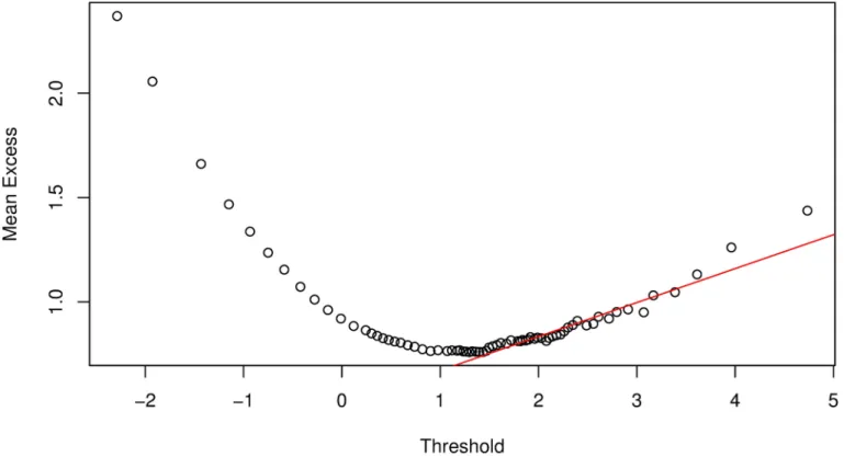
The choice of a thresholdϑis an important step in the POT method becauseEq (34)is dependent onϑand the number of points (i.e., exceedances) aboveϑsince the parameters are estimated based on the exceedances. Thus, it is very important to find the proper threshold value. There is no clear-cut or wholly satisfactory method to determine a proper threshold that has been determined to date. [57] developed a semi-parametric estimator for the tails of the distribution that estimated the threshold of the bootstrap approximation of the mean square error (MSE) of the tail index and by minimising MSE through the choice of the threshold. [58] further used a two-step subsample bootstrap method to determine the threshold that mini-mised the asymptotic MSE. [59,60] propose graphical tools to identify the proper threshold known as the Hill plot and the mean excess plot, respectively. In this paper, we use the mean excess plot and propose its extension, which wee call ahybridmethod as will be discussed later.

A mean excess function ofxover a certain thresholdϑis defined as

eðWÞ ¼Eðx Wjx>WÞ ¼sþxW

1 x : ð36Þ A property of the GPD states that if the excess distribution ofxgiven a thresholdϑ0be a GPD with shape parameterξand scale parameterψ(ϑ0), then for any random thresholdϑ>ϑ0, the excess distribution over the thresholdϑhas a GPD with shape parameterξand scale parameter

ψ(ϑ) =ψ(ϑ0) +ξ(ϑ−ϑ0), where 0<ξ<1 [55]. Then

eðWÞ ¼Eðx Wjx>WÞ ¼cðW0Þ þxðW W0Þ

1 x ; ð37Þ which is a linear function ofϑ−ϑ0with slopeξ/(1−ξ) forϑ>ϑ0. From the ordered sample {xi}, we calculate and plot the mean excess function, i.e.,Eq (37)against each chosenϑiforϑi>

ϑ0. The thresholdϑis then identified as the lowest point on the mean excess plot above which the graph appears to be approximately linear. However, the choice ofϑfrom the mean excess plot is subjective [8,55] and might differ from one bank to another using the same data because of different risk tolerances. Differentϑvalues will give different estimates of the shape

and scale parameter. A very high threshold will result in too few data points in the left tail for any meaningful statistical analysis. In contrast, a very low threshold will result in a number of data points above the threshold lying close to the body of the sample data. This will result in a poor approximation because the GPD is a limiting distribution asϑ! 1; data beyond the threshold will deviate from the GPD since the GPD is not a good approximation for the body of the sample data [8,56]. We propose ahybridmethod for selecting a proper threshold value that will significantly diminish the possibility of differentϑvalues with the same data.

Data

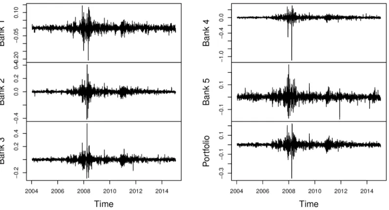
The data employed in this analysis consist of 2870 daily observations of stock prices actively traded on the London Stock Exchange. The stocks belong to the banking sector and of the top five banks in the UK, i.e., HSBC Holdings, Lloyds Banking Group, Barclays Plc., Royal Bank of Scotland Group, and Standard Chartered Plc. We refer to these banks as Bank 1, Bank 2, Bank 3, Bank 4, and Bank 5, respectively. The motivation for selection of these banks is to test the reliability of the proposed VaR models for the top UK banks in periods of distress. Therefore, our data covers the period from 31 December 2004 to 31 December 2015, covering the 2008 global financial crisis and the 2011 European financial crisis. All data are from DataStream.

In some literature the stability in financial systems is measured using a portfolio consisting of several banks (i.e., by considering the dependence among the banks), while other studies focus on individual banks. This paper considers both measures. Therefore, by using the stock prices for each bank, we calculate the log-return series and apply risk factor mappings to con-struct a simulated portfolio of returns for all banks as follows: Consider a portfolio consisting ofNrisk factors represented in vector form asSN= (s1t,. . .,sNt), the log-returnsrt, are calcu-lated as rt¼ log S1;tþt S1;t ! ;. . .;log SN;tþt SN;t ! " # ¼ ðr1t;. . .;rNtÞ: ð38Þ

Let Inv be the total amount invested in the portfolio,xibe the fraction of the total invest-ment invested in stocki,ri,tis the return of stockiat timet, then the weight applied tori,tis the fraction of the portfolio invested in stockicalculated aswi ¼

xi

Inv. Since the stocks are all from

banks of almost the same strength (i.e., the top five banks in the UK), we may assume equal weights. Therefore, the expected return on the portfolio at timetis given by

Rp;t¼EðRp;tÞ ¼ XN i¼1 wiEðri;tÞ; XN i¼1 wi¼1; ð39Þ

which is a weighted average of the return on the individual stocks in the portfolio.

Fig 1shows time plots of the log-return series and the portfolio; this shows evidence of vola-tility clustering in the return series. From the figure, we can also see the effects of the 2008 global financial crisis and the 2011 European financial crisis.

Table 1presents summary statistics of the data. We see from the table that the log-return series for each bank and the portfolio are far from being normally distributed as indicated by their high excess kurtosis and skewness. Furthermore, Jarque-Bera normality tests, Ljung-Box tests on the squared residualsa2

i;t; whereai,t=ri,t−μi(μibeing the unconditional mean), and a Lagrange multiplier tests for autoregressive conditional heteroscedasticity (ARCH LM test) on the residualsai,t, as described in [55,61,62], are significant at 5% level.

Results

Modelling the marginal distributions of volatility equations

As noted, the log-return series are leptokurtic and skewed. Thus, to capture the tail distribu-tion and the dynamics of fluctuadistribu-tions in the time series data, we consider a single-state,k= 1 and two-state,k= {1, 2} Markov Switching GARCH specifications. The underlying volatility model is a GJR-GARCH(1,1) model with skewed Student’s-tdistribution. Since we use just one variance specification (i.e., GJR-GARCH), the two-state Markov Switching GARCH is generated by setting the number of regimes in the conditional distribution to 2. For the single-state, the length of the variance specification is equal to the length of the conditional distribu-tion, which is 1 (see [14]). Also note that the single-state Markov Switching GJR-GARCH(1,1)

Fig 1. Time plots of the log-return series. Plots show the presence of volatility clustering in the log-return data.

https://doi.org/10.1371/journal.pone.0198753.g001

Table 1. Summary statistics of daily log-returns and portfolio return series.

Bank 1 Bank 2 Bank 3 Bank 4 Bank 5 Portfolio

Mean -0.0001 -0.0004 -0.0003 -0.0010 -0.0001 -0.0004 Variance 0.0003 0.0011 0.0010 0.0015 0.0006 0.0006 Std. deviation 0.0171 0.0328 0.0321 0.0388 0.0244 0.0239 Skewness -0.3367 -1.0549 1.4387 -8.4013 0.3161 -0.7549 Excess kurtosis 16.9080 37.2754 40.2179 235.5263 13.0850 28.6129 https://doi.org/10.1371/journal.pone.0198753.t001

model corresponds to GJR-GARCH(1,1) model without regime change. Therefore, we simply refer to the single-state and two-state Markov Switching GJR-GARCH(1,1) models as

GJR-GARCH(1,1) and MS-GJR-GARCH(1,1) models, respectively (see [14]). GARCH param-eters are estimated using Bayesian statistics as follows: (i) We assign a prior distribution with initial hyperparameters and generate MCMC simulations of 40000 draws; (ii) if convergence is attained, we discard the first 20000 draws and select only the 10thdraw from each chain such that auto-correlation between draws is reduced to almost zero. We merge the two chains together to obtain a sample data set of 2000 observations. (iii) If convergence is not attained, repeat (i) using parameter estimates from the previous draw as the hyperparameters to increase the chance of convergence. The mean value of each parameter with respect to its respective posterior distribution is the optimal parameter estimate of the Bayesian

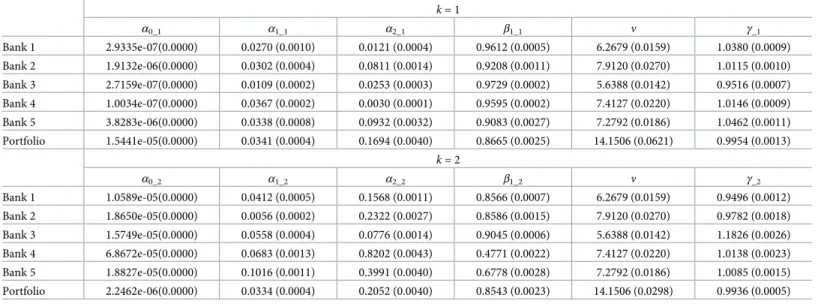
GJR-GARCH(1,1) and Bayesian MS-GJR-GARCH(1,1) models with skewed Student’s-t distri-butions. Estimation results are presented in Tables2and3with standard errors in parenthesis. For MS-GJR-GARCH(1,1) model, the degrees of freedom parameter,νis fixed across the regimes.

Table 2. Parameter estimates following Bayesian GJR-GARCH(1,1) model with skewed Student’s-t distribution.

α0 α1 α2 β1 ν γ Bank 1 7.0531e-06(0.0000) 0.0508(0.0010) 0.1001(0.0000) 0.8488(0.0002) 5.8153 (0.0114) 1.0067(0.005) Bank 2 1.4764e-6(0.0000) 0.0509(0.0000) 0.1001(0.0000) 0.8570(0.0001) 6.4085 (0.0133) 1.0014 (0.0005) Bank 3 7.0777e-06(0.0000) 0.0511(0.0000) 0.1001(0.0000) 0.8716(0.0001) 6.1691 (0.0118) 1.0009 (0.0005) Bank 4 9.4281e-06(0.0000) 0.0511(0.0000) 0.1002(0.0000) 0.8688(0.0001) 5.9166 (0.0111) 1.0160 (0.0005) Bank 5 2.0683e-05(0.0000) 0.0508(0.0000) 0.1002(0.0000) 0.8321(0.0002) 6.3657 (0.0138) 1.0266 (0.0005) Portfolio 5.4112e-06(0.0000) 0.0510(0.0000) 0.1002(0.0000) 0.8670(0.0001) 9.4379 (0.0298) 0.9936 (0.0005) Note: Standard errors in parentheses.

https://doi.org/10.1371/journal.pone.0198753.t002

Table 3. Parameter estimates for two-state MS-GJR-GARCH(1,1) model with skewed Student’s-t distribution.

k= 1 α0_1 α1_1 α2_1 β1_1 ν γ_1 Bank 1 2.9335e-07(0.0000) 0.0270 (0.0010) 0.0121 (0.0004) 0.9612 (0.0005) 6.2679 (0.0159) 1.0380 (0.0009) Bank 2 1.9132e-06(0.0000) 0.0302 (0.0004) 0.0811 (0.0014) 0.9208 (0.0011) 7.9120 (0.0270) 1.0115 (0.0010) Bank 3 2.7159e-07(0.0000) 0.0109 (0.0002) 0.0253 (0.0003) 0.9729 (0.0002) 5.6388 (0.0142) 0.9516 (0.0007) Bank 4 1.0034e-07(0.0000) 0.0367 (0.0002) 0.0030 (0.0001) 0.9595 (0.0002) 7.4127 (0.0220) 1.0146 (0.0009) Bank 5 3.8283e-06(0.0000) 0.0338 (0.0008) 0.0932 (0.0032) 0.9083 (0.0027) 7.2792 (0.0186) 1.0462 (0.0011) Portfolio 1.5441e-05(0.0000) 0.0341 (0.0004) 0.1694 (0.0040) 0.8665 (0.0025) 14.1506 (0.0621) 0.9954 (0.0013) k= 2 α0_2 α1_2 α2_2 β1_2 ν γ_2 Bank 1 1.0589e-05(0.0000) 0.0412 (0.0005) 0.1568 (0.0011) 0.8566 (0.0007) 6.2679 (0.0159) 0.9496 (0.0012) Bank 2 1.8650e-05(0.0000) 0.0056 (0.0002) 0.2322 (0.0027) 0.8586 (0.0015) 7.9120 (0.0270) 0.9782 (0.0018) Bank 3 1.5749e-05(0.0000) 0.0558 (0.0004) 0.0776 (0.0014) 0.9045 (0.0006) 5.6388 (0.0142) 1.1826 (0.0026) Bank 4 6.8672e-05(0.0000) 0.0683 (0.0013) 0.8202 (0.0043) 0.4771 (0.0022) 7.4127 (0.0220) 1.0138 (0.0023) Bank 5 1.8827e-05(0.0000) 0.1016 (0.0011) 0.3991 (0.0040) 0.6778 (0.0028) 7.2792 (0.0186) 1.0085 (0.0015) Portfolio 2.2462e-06(0.0000) 0.0334 (0.0004) 0.2052 (0.0040) 0.8543 (0.0023) 14.1506 (0.0298) 0.9936 (0.0005) Note: Standard errors in parentheses. Degrees of freedom parameter,νis fixed across the regimes.

ApplyingEq (2), we then obtain a matrixS, which consists of the filtered marginal stan-dardised residuals,f_i;tg

T

t¼1, of the overall process for the MS-GJR-GARCH(1,1) model and

GJR-GARCH(1,1) model. That is

S_i;t¼ ðri;tÞ h 1 2 D_i;t;i;t ; i¼1;. . .;N; t¼1;. . .;T: ð40Þ

The ARCH LM test and Ljung-Box test on the standardised residuals and standardised squared residuals, respectively, for lags 5 and 10 are presented inTable 4. For the

GJR-GARCH(1,1) model, there still exist some serial correlation in the standardised residuals of bank 4. For MS-GJR-GARCH(1,1) model, there is no evidence of an ARCH effect or serial correlations in the standardised residuals.

Modelling dependence with copulas

We model the dependence structure among the stock returns using copula functions. Copula parameters are estimated by the canonical maximum likelihood (CML) method [41]. This entails the use of pseudo-observations of the standardised residuals to estimate the marginals. We then estimate the copula parameters by inversion of Kendall’sτ, which is one of the most commonly used invariant measures and has been proven to provide more efficient ways of estimating correlations [63,64]. The copula that fits the data best is selected by maximum like-lihood estimation (MLE) method by maximising the likelike-lihood function

^

C2¼ArgMaxC2 XT

t¼1

lncðF^1ðX1tÞ;. . .;F^nðXntÞ;C2Þ; ð41Þ

whereC^2are estimates of the copula parameters. The estimated copula parameters are

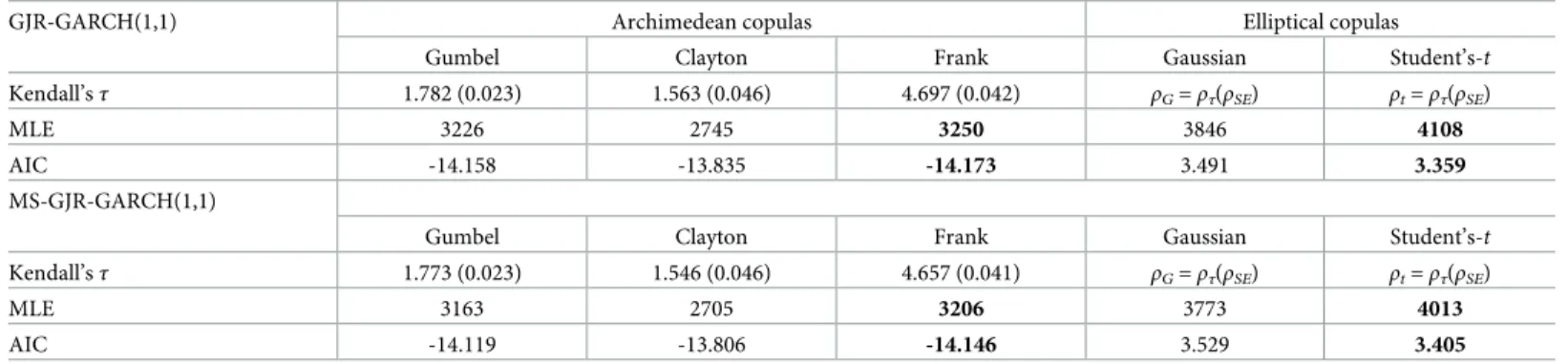
reported inTable 5, along with their Akaike information criterion (AIC) values. For both models, Frank and Student’s-tcopulas are selected from each copula family based on the high-est MLE values. FromTable 5, the same copula types have been selected based on the AIC val-ues (the copula with the smallest AIC value is preferred). Note that Gaussian copula gives a higher MLE value compared to the Archimedean copulas but also higher AIC value.Table 6

Table 4. ARCH LM test on the standardised residuals and Ljung-Box test on the standardised squared residuals fork = 1. The null hypothesis of no ARCH effect or serial correlation is rejected at 5% significant level for Bank 4.

k= 1 ARCH LM test Ljung-Box test

Bank 1 Bank 2 Bank 3 Bank 4 Bank 5 Bank 1 Bank 2 Bank 3 Bank 4 Bank 5

LM(5) 2.21 2.35 2.96 17.78 4.01 Q(5) 2.24 2.35 2.95 17.65 4.11

p-value 0.820 0.800 0.706 0.003 0.548 p-value 0.815 0.799 0.707 0.003 0.534

LM(10) 10.26 4.13 7.04 18.62 6.79 Q(10) 9.92 4.14 7.17 18.57 6.89

p-value 0.820 0.942 0.722 0.045 0.745 p-value 0.447 0.941 0.710 0.046 0.736

k= {1, 2} ARCH LM test Ljung-Box test

Bank 1 Bank 2 Bank 3 Bank 4 Bank 5 Bank 1 Bank 2 Bank 3 Bank 4 Bank 5

LM(5) 2.164 2.29 8.74 5.31 3.06 Q(5) 2.13 2.22 8.60 5.30 10.56

p-value 0.826 0.807 0.120 0.379 0.690 p-value 0.831 0.818 0.126 0.380 0.061

LM(10) 6.01 3.75 13.39 5.83 5.30 Q(10) 5.98 3.70 13.27 5.88 12.71

p-value 0.815 0.958 0.203 0.829 0.870 p-value 0.817 0.960 0.209 0.826 0.240 Note: Fork= 1, we have a GJR-GARCH(1,1) model, and fork= {1, 2}, we have a MS-GJR-GARCH(1,1) model.

shows the Kendall’sτfor Gaussian and Student’s-tcopula parameter estimates. Thus, the Gaussian copula is not a good fit for the data. The analysis continues based on the selected cop-ulas. Next, we specify the desired marginal distributions, which we set to Student’s-t distribu-tion, and using the estimated copula parameters, we generate 10000 simulations to obtain a new matrix of marginal standardised residuals

^

S¼ fz_i;jg; j¼1;. . .;T; i¼1;. . .;N; ð42Þ which is free from assumptions of normality and linear correlations. To confirm this, we employ a multivariate ARCH test based on the Ljung-Box test statistics

QkðmÞ ¼T 2X m i¼1 1 T ib 0 iðρ^ 1 0 ρ^ 1 0 Þbiw 2 k2ðmÞ; ð43Þ

and its modificationQr

kðmÞ, known as a robust test, on the log returns at 5% significance level, wheremis the number of lags of cross-correlation matrices used in the tests,kis the dimen-sion ofri,t,Tis the sample size,bi¼vecð^r

0

iÞwithρ^jbeing the lag-jcross-correlation matrix of

Table 5. Copula parameter estimates are based on inversion of Kendall’sτ following CML estimation method.

GJR-GARCH(1,1) Archimedean copulas Elliptical copulas

Gumbel Clayton Frank Gaussian Student’s-t

Kendall’sτ 1.782 (0.023) 1.563 (0.046) 4.697 (0.042) ρG=ρτ(ρSE) ρt=ρτ(ρSE)

MLE 3226 2745 3250 3846 4108

AIC -14.158 -13.835 -14.173 3.491 3.359

MS-GJR-GARCH(1,1)

Gumbel Clayton Frank Gaussian Student’s-t

Kendall’sτ 1.773 (0.023) 1.546 (0.046) 4.657 (0.041) ρG=ρτ(ρSE) ρt=ρτ(ρSE)

MLE 3163 2705 3206 3773 4013

AIC -14.119 -13.806 -14.146 3.529 3.405

Note: Standard errors in parentheses. The best copula for modeling dependence among the risk factors is that with the highest MLE value or smallest AIC value (in bold).

https://doi.org/10.1371/journal.pone.0198753.t005

Table 6. Kendall’sτ; ρτ(ρSE) for Gaussian and Student’s-t copula parameter estimates.

Bank 1 Bank 2 Bank 3 Bank 4 Bank 5

GJR-GARCH(1,1) Bank 1 1 Bank 2 0.6230 (0.013) 1 Bank 3 0.5521 (0.015) 0.7054 (0.011) 1 Bank 4 0.5741 (0.014) 0.7262 (0.011) 0.7176 (0.011) 1 Bank 5 0.6383 (0.013) 0.6027 (0.014) 0.5437 (0.015) 0.5460 (0.015) 1 MS-GJR-GARCH(1,1) Bank 1 1 Bank 2 0.6257 (0.013) 1 Bank 3 0.5544 (0.015) 0.7074 (0.011) 1 Bank 4 0.5779 (0.015) 0.7282 (0.011) 0.7225 (0.011) 1 Bank 5 0.6437 (0.012) 0.6075 (0.014) 0.5439 (0.015) 0.5483 (0.015) 1 Note: Standard errors in parentheses.

r2

i;t. The modificationQ r

kðmÞinvolves discarding those observations from the return series whose corresponding standardised residuals exceed 95thquantile in order to reduce the effect of heavy tails. The motivation forQr

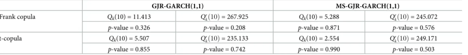
kðmÞtest is thatQk(m) may fare poorly in finite samples when the residuals of the time series,ri,t, have heavy tails [45]. The tests show no evidence of conditional heteroscedasticity lagsm= 10;Table 7.

We follow the approach by [9] and apply the POT method of EVT to each of the marginal distributions of {zi,t} (i.e.,Eq (42)) to obtain theqthquantile,VaR(Z)qof the noise variables for VaR estimation. Let {χi,τ} be the negative variables of the marginal distributions of {zi,t} such that {χi,τ}{zi,t}. Then, from the ordered sample of {χi,τ}, we calculate and plot the mean excess function to help identify the threshold. As an example, Figs2and3are mean excess function plots for Bank 1 following the Bayesian GJR-GARCH(1,1) Student’s-tand Frank cop-ula models. The plots suggest us to select threshold values of about 1.3 and 1.4 for Figs2and3, respectively, which are the lowest points on the graphs above which the graph appears to be

Table 7. Multivariate ARCH test on {zi,j} shows no evidence of conditional heteroscedasticity.

GJR-GARCH(1,1) MS-GJR-GARCH(1,1)

Frank copula Qk(10) = 11.413 Qrkð10Þ= 267.925 Qk(10) = 5.288 Qrkð10Þ= 245.072

p-value = 0.326 p-value = 0.208 p-value = 0.871 p-value = 0.576 t-copula Qk(10) = 5.507 Qrkð10Þ= 235.133 Qk(10) = 2.554 Qrkð10Þ= 249.171

p-value = 0.855 p-value = 0.742 p-value = 0.990 p-value = 0.503 https://doi.org/10.1371/journal.pone.0198753.t007

Fig 2. Mean excess function plot for Bank 1 following analysis with Bayesian GJR-GARCH(1,1) Student’s-t copula model. https://doi.org/10.1371/journal.pone.0198753.g002

approximately linear. However, if we select these points as the threshold values, we will have 1402 exceedances forFig 2and 1039 exceedances forFig 3, which are too many compared to the size of the data (i.e.,T= 10000). The number of exceedances thus lie towards the body of the data, which will inevitably result in a poor approximation of the GPD parameters and hence lead to inaccuracies in the VaR estimate. In addition, the threshold selection method is very subjective and will be different from one analyst to the other based on their preferences.

We propose an extension to the mean excess plot for threshold selection; thehybrid

method. That is, from the mean excess plot, we identify the lowest point, making the graph appears approximately linear, a pointϑ0. We then insert a tangent line fromϑ0through the rest of the pointsϑi, whereϑi>ϑ0; seeFig 4. Since the tangent to a linear curve is the tangent itself and the mean excess function is a linear function of the threshold, we take an average of the set of points that touches the tangent line as the threshold value, a pointϑ_{. This pointϑ}

will lead to a better approximation of VaR estimates thanϑ0because the inference is restricted to the left tail. Apart from better approximation of VaR estimates, this method significantly reduces the probability of having different VaR estimates for the same data and also the proba-bility of selecting a very low or very high threshold value. Letϑi=ϑ1,. . .,ϑℏbe a set of points

that touches the tangent line, then we obtain the value ofϑas

W ¼1 ℏ Xℏ i¼1 W_i; W_iW₀; ð44Þ

whereℏis the number of points in the set.

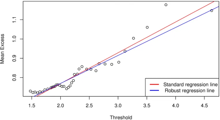
Fig 3. Mean excess function plot for Bank 1 following analysis with Bayesian GJR-GARCH(1,1) Frank copula model.

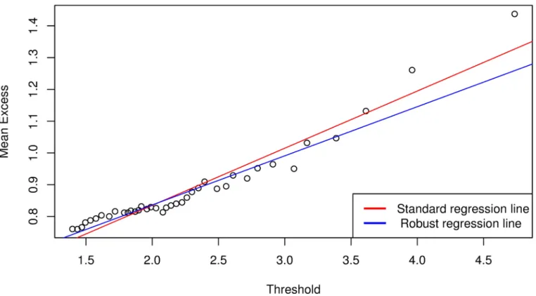
It can be seen inFig 4that the points touching the tangent line, i.e.,ϑ0, are too compact and might lead us to miss some important points. A better way for selecting these points is by fit-ting a regression line

^

y¼b0þb1x; ð45Þ

which is based on the least square method to the pointsfW_igℏ_i¼1, where^yis the estimate of the

dependent variable, andxis the independent variable with interceptb0and slopeb1. In the presence of heteroscedasticity and outliers, it may be advantageous to consider fitting a robust regression line. Robust regression methods are not influenced by outliers, and are also very useful when there are problems with heteroscedasticity in the data set. This method is demon-strated for Bank 1 in Figs5and6, which illustrates a comparison between simple linear and robust regression methods. It can be seen that the regression lines for standard regression models are affected by outliers in the left tails of the mean excess plots, hence a robust regres-sion model is more reliable.

Following the above analysis, we obtained a threshold value of 2.2448 and 333 exceedances forFig 5, and 2.6476 and 176 exceedances forFig 6. The analysis are restricted to the tails and the data is sufficient to allow for reasonable statistical inferences with EVT. Tables8and9

presents the POT parameter estimates and the forecast VaR estimates. The portfolio VaR esti-mates,VaRp

qðZÞ, based on the individual bank’s VaR estimates and confidence level are also reported.VaRp

qðZÞis computed using the risk formula

VaRp qðZÞ ¼ XN i¼1 w2 iVaR 2 q;iðZÞ þ2wiwj XN i<j r_ijVaRq;iðZÞVaRq;jðZÞ ! 1 2; XN i¼1 wi¼1; ð46Þ

Fig 4. Mean excess function plot demonstrating thehybrid method for threshold selection. https://doi.org/10.1371/journal.pone.0198753.g004

whereρi,jis the Pearson cross-correlation coefficient between the returns of theith andjth stocks. As noted, the overall risk measures are quite stable for both models and different thresholds indicating that the model has effectively captured the dynamics of fluctuations in the left tails of the return distributions. This claim may be validated through back-testing the model. We can also see the effect of diversification on the risk of the individual banks on the portfolio VaR. EmployingEq (46), the one step ahead VaR is then calculated as

VaRpq;t¼VaRpqðZÞ^h 1 2

D_t;tþ1: ð47Þ

Note thath^12

D_t;tþ1is the one-step-ahead conditional volatility forecast of the overall conditional

variance for the portfolio at timet+ 1 for statek,Δtis a Markov chain as defined in Eqs (1) and (2), but forRpis byEq (39). That is,Rp;tjðDt¼k;Ot 1Þand the parameters are sampled

from the posterior distribution using MH algorithm.

Figs7–10show time plots of profit and loss (P&L) of the portfolio return series and fore-casts portfolio VaR estimates at 99% and 95% confidence levels. A visual observation of the plots suggests that the VaR models perform quite well in capturing the dynamics in the portfo-lio return series.

Fig 5. Mean excess function plot following analysis with Bayesian GJR-GARCH(1,1) Student’s-t copula model for the number of exceedances above ϑ0. A

reliable threshold is calculated by taking an average of the set of points that touches the robust regression line. The standard regression line is affected by outliers in the left tail.

Table 8. POT parameter estimates,VaRq(Z) and VaRp

qðZÞfollowing Bayesian GJR-GARCH(1,1) Frank and Student’s-t copula-EVT models.

Parameters VaRq(Z)

ξ ψ(ϑ_{) ϑ Nϑ μ σ 99% 95%}

Student’s-tcopula: Bank 1 0.1660 0.7143 2.2448 333 0.3881 0.4061 3.1958 1.9640 Bank 2 0.2239 0.6479 2.4624 218 0.7974 0.2750 3.0141 1.9716 Bank 3 0.1838 0.6353 2.2321 356 0.6481 0.3441 3.1407 2.0229 Bank 4 0.1273 0.7301 2.4687 271 0.3567 0.4612 3.2448 2.0385 Bank 5 0.1465 0.7135 2.3293 287 0.3538 0.4242 3.1428 1.9489 VaRp qðZÞ 2.5862 1.6282

Frank copula: Bank 1 0.1019 0.7239 2.6476 176 0.2503 0.4796 3.0688 1.9305 Bank 2 0.0497 0.7489 2.4331 235 -0.1297 0.6216 3.0867 1.8781 Bank 3 0.0390 0.7892 2.6040 223 -0.1855 0.6804 3.2469 1.9767 Bank 4 0.2073 0.6862 2.5407 217 0.7266 0.3102 3.1174 2.0147 Bank 5 0.1062 0.6892 3.1337 105 0.6440 0.4249 3.1674 2.1425 VaRp qðZÞ 2.5410 1.6459

Note: Estimations for a time horizon of 1 day atq= (99%, 95%) confidence level. The risk measures are quite stable for different thresholds and copula functions indicating that the VaR models have successfully capture the dynamics of fluctuations in the left tails.

https://doi.org/10.1371/journal.pone.0198753.t008

Fig 6. Mean excess function plot following analysis with Bayesian GJR-GARCH(1,1) Frank copula model for the number of exceedances aboveϑ0.

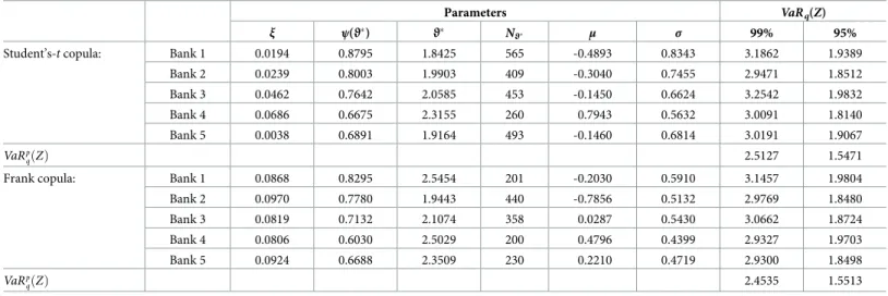
Table 9. POT parameter estimates,VaRq(Z) and VaRp

qðZÞfollowing Bayesian MS-GJR-GARCH(1,1) Frank and Student’s-t copula-EVT models.

Parameters VaRq(Z)

ξ ψ(ϑ_{) ϑ Nϑ} μ σ 99% 95%

Student’s-tcopula: Bank 1 0.0194 0.8795 1.8425 565 -0.4893 0.8343 3.1862 1.9389 Bank 2 0.0239 0.8003 1.9903 409 -0.3040 0.7455 2.9471 1.8512 Bank 3 0.0462 0.7642 2.0585 453 -0.1450 0.6624 3.2542 1.9832 Bank 4 0.0686 0.6675 2.3155 260 0.7943 0.5632 3.0091 1.8140 Bank 5 0.0038 0.6891 1.9164 493 -0.1460 0.6814 3.0191 1.9067 VaRp qðZÞ 2.5127 1.5471

Frank copula: Bank 1 0.0868 0.8295 2.5454 201 -0.2030 0.5910 3.1457 1.9804 Bank 2 0.0970 0.7780 1.9443 440 -0.7856 0.5132 2.9769 1.8480 Bank 3 0.0819 0.7132 2.1074 358 0.0287 0.5430 3.0662 1.8724 Bank 4 0.0806 0.6030 2.5029 200 0.4796 0.4399 2.9327 1.9703 Bank 5 0.0924 0.6688 2.3509 230 0.2210 0.4719 2.9300 1.8498 VaRp qðZÞ 2.4535 1.5513

Note: Estimations for a time horizon of 1 day atq= (99%, 95%) confidence level. The risk measures are quite stable for different thresholds and copula functions indicating that the VaR models have successfully capture the dynamics of fluctuations in the left tails.

https://doi.org/10.1371/journal.pone.0198753.t009

Fig 7. Forecasts daily VaR estimates and daily profit and loss (P&L) plots for an investment in a portfolio consisting of all banks following Bayesian GJR-GARCH(1,1) Student’s-t copula EVT VaR model.

Fig 8. Forecasts daily VaR estimates and daily profit and loss (P&L) plots for an investment in a portfolio consisting of all banks following Bayesian GJR-GARCH(1,1) Frank copula EVT VaR model.

https://doi.org/10.1371/journal.pone.0198753.g008

Fig 9. Forecasts daily VaR estimates and daily profit and loss (P&L) plots for an investment in a portfolio consisting of all banks following Bayesian MS-GJR-GARCH(1,1) Student’s-t copula EVT VaR model.

Model checking

The reliability of the VaR model is often tested by performing back-testing. This involves com-paring the estimated VaRs for a given time horizon and observation period to the subsequent returns and recording the number of days in which the loss on the portfolio exceeds VaR. The number of daysT1in which the loss on the portfolio exceeds VaR is recorded as the number of exceptions or failures. Too many exceptions imply that the VaR model underestimates the level of risk, and too few exceptions imply the model overestimates risk. For the VaR model to be accepted as a reliable risk measure, the number of exceptions produced for any given obser-vation period should satisfy the unconditional coverage (UC) and independent (IND) proper-ties. We define an indicator function on the exceptions at timetas

I_tð1 qÞ ¼I_fL t>VaRpq;tg¼ ( 1; if Lt>VaR p q;t 0; otherwise; ð48Þ

where the indicator function equal to 1 when the loss on the portfolioLtexceedVaR p

q;t, and 0 if otherwise; note thatqis the choice of confidence level. For the UC property,

Pr½I_tð1 qÞ ¼1Š 1 q;8_t; i.e., the number of exceptions should be reasonably close to

Tw(1−q)%, depending on the choice ofq, and should follow a binomial distribution.Twis the size of the window over which back-testing is conducted. For the IND property, the exceptions produced on dayt− 1 should be independent of exceptions produced on daytand evenly spread over time.

Fig 10. Forecasts daily VaR estimates and daily profit and loss (P&L) plots for an investment in a portfolio consisting of all banks following Bayesian MS-GJR-GARCH(1,1) Frank copula EVT VaR model.

In this study, we use several back-testing methods to test the accuracy of the proposed VaR models. The most common are the Kupiec’s proportion of failures (POF) test for the UC [65], Christoffersen’s test for the UC and IND [66], Engle and Manganelli’s Dynamic Quantile (DQ) test [67], and Santos and Alves’ new class of independence test [68]. We also consider the Baseltraffic lighttest proposed by the Basel Committee on Banking and Supervision (BCBS) [69].

Kupiec defined an approximate 95% confidence region whereby the number of exceptions produced by the VaR model must lie within this interval for it to be considered a reliable risk measurement model. The test is based on the likelihood ratio

LRUC¼ 2ln qT0_{ð1 qÞ}T1 1 T1 T_w T0 _T 1 T_w T1 w 2 1; ð49Þ

whereT0=Tw−T1. Under the UC, the null hypothesis forLRPOFisH0:E½Itð1 qފ ¼ T1 T_w¼

1 qagainstHa:E½Itð1 qފ ¼ T1

Tw6¼ ð1 qÞ. The VaR model is rejected if

LRPOF>w

2

1 ¼3:841.

A study by [66] extended Kupiec’s POF test to test the independence of conditional cover-age. Under the null hypothesis that the number of exceptions produced are independent and evenly spread over time,π01=π11=πwith likelihood ratio

LRIND¼ 2ln ð1 pÞðT00þT10ÞpðT01þT11Þ ð1 p01Þ T00_pT01 01ð1 p11Þ T10_pT11 11 w2 1; ð50Þ

whereTij, withi,j= 0(noviolation), 1(violation), is the number of observed events with thejth event followingith, andπ01,π01andπare estimates of the probabilities ofTi,j[70]. The model is rejected for the independent property ifLRIND>w

2

1¼3:841. Christoffersen conditional

cov-erage test is a joint test of Kupiec’s POF test and the IND that test both properties of UC and IND instantaneously. The conditional coverage test has a likelihood ratio

LRCC ¼LRPOFþLRINDw

2

2: ð51Þ

The hypothesis is Pr½I_tð1 qÞ ¼1jO_t 1Š ¼1 q;8tagainst

Pr½I_tð1 qÞ ¼1jO_t 1Š 6¼1 q;8t, whereOt−1is the information available on dayt− 1. The model is rejected for the conditional coverage property ifLRCC>w

2

2 ¼5:99.

TheDQtest utilises the criterion that the number of exceptions produced on daytshould be independent of the information available at dayt− 1. The function is defined as

Hitt¼IðLt< VaR p q;tÞ ð1 qÞ ¼ ( q; if Lt<VaR p q;t ð1 qÞ; otherwise: ð52Þ

TheHittfunction assumes the valueqwhen the loss on the portfolio at timetis less than

VaRpq;t, and−(1 −q) otherwise. As explained in [67], clearly E[Hitt] = 0, E[Hitt|Ot−1] = 0 and Hittmust be uncorrelated with its own lagged values. The test statistics is given by

DQ¼ðHit 0 tXt½X 0 tXtŠ 1 X0tHittÞ ð1 qÞq ; ð53Þ

whereXtis a vector containing all values ofHitt,VaRpq;tand its lags. Under the null hypothesis E[Hitt] = 0 and E[Hitt|Ot−1] = 0,HittandXtare orthogonal andHittmust be uncorrelated with its own lagged values [67,71]. TheDQtest is easy to perform, and does not depend on the

estimation procedure; all that is needed is a series of VaRs and the corresponding values of the portfolio returns [67]. In this study, we follow [67,72,73] to use a constant, four lagged values ofHitt.

In Santos and Alves’ new class of independence test [68], we first define the duration between two consecutive exceptions asDi=ti−ti−1, wheretidenotes the time of exception numberi; andt0= 0 implies thatD1is the time until the first exception. We denote a sequence ofNdurations byfDig

N

i¼1, where the order statistics areD1:N. . .DN:N. The test statistics is defined as

TN;½N=2Š¼ log2

DN:N 1

D½N=2Š:N

logN: ð54Þ

See [68] for more details on this test.

Finally, BCBS developed a set of requirements that the VaR model must satisfy for it to be considered a reliable risk measure and proposed the Baseltraffic lighttest. That is, (i) VaR must be calculated with 99% confidence, (ii) back-testing must be done using a minimum of a one year observation period and must be tested over at least 250 days, (iii) regulators should be 95% confident that they are not erroneously rejecting a valid VaR model, and (iv) Basel speci-fies a one-tailed test —it is only interested in the underestimation of risk [74]. [2] summarises the acceptance region for the Baseltraffic lightapproach to back-testing VaR models.

We use out-of-sample data ofm=T−nobservations for back-testing; thus we have

n= 1869 sample of the return observations for VaR estimation procedure containing the 2008 global financial crisis period, andm= 1000 of return observations for back-testing. VaR is then estimated following a rolling window approach. The out-of-sample data is further divided into blocks of 250, 500, and 1000 trading days to observe how the models behave for both lon-ger and shorter observation periods. The division of out-of-sample data is also employed to meet the BCBS requirements.Table 10presents the expected and observed number of excep-tions produced following each model for a portfolio consisting of all five banks. At 99% confi-dence level and 250 trading days, the MS-GJR-GARCH(1,1) copula EVT VaR model

registered 3 exceptions for a single-state and 0 exceptions for a two-state MS-GJR-GARCH (1,1) model. Thus, following Basel rules for back-testing, the VaR models passed the reliability test and are placed in the green zone. Back-testing results based onLRUC,LRIND,LRCC,DQ,

Table 10. Expected versus observed number of exceptions following Bayesian MS-GJR-GARCH(1,1) and GJR-GARCH(1,1) copula-EVT VaR model.

250 500 1000

1% 5% 1% 5% 1% 5%

Expected exceptions 2.5 12.5 5 25 10 50

GJR-GARCH(1,1) Observed exceptions fort-copula 3 11 4 26 8 57

Coverage rate 0.012 0.044 0.008 0.052 0.008 0.057

Observed exceptions for Frank copula 3 11 5 24 9 55

Coverage rate 0.012 0.044 0.010 0.048 0.009 0.055

MS-GJR-GARCH(1,1) Observed exceptions fort-copula 0 6 0 15 0 33

Coverage rate 0.000 0.024 0.000 0.030 0.000 0.033

Observed exceptions for Frank copula 0 6 0 14 0 32

Coverage rate 0.000 0.024 0.000 0.028 0.000 0.032

Note: Out-of-sample data is divided into blocks of 250, 500, and 1000 observation periods, time horizon of 1 day. The coverage rateT1

Tw1 q. https://doi.org/10.1371/journal.pone.0198753.t010