XIX Ciclo del Dottorato di Ricerca in Ingegneria e Architettura
An Evolutionary Multi-Objective
Optimization Framework for Bi-level
Problems
Settore scientifico-disciplinare
MAT/09 - RICERCA OPERATIVA
COORDINATORE:
D
iego Micheli
SUPERVISORE DI TESI:
L
orenzo Castelli
CO-SUPERVISORE:
A
lessandro Turco
DOTTORANDO:
S
tefano Costanzo
ANNO ACCADEMICO 2015 - 2016
/'
C:-Y
,,,n
�
n
\
tfL,o,...e,,._
+o
La-i_G
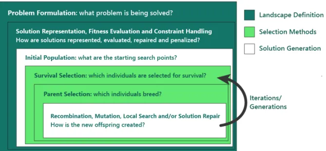
enetic algorithms (GA) are stochastic optimization methods inspired by the evolution-ist theory on the origin of species and natural selection. They are able to achieve good exploration of the solution space and accurate convergence toward the global optimal solution. GAs are highly modular and easily adaptable to specific real-world problems which makes them one of the most efficient available numerical optimization methods.This work presents an optimization framework based on the Multi-Objective Genetic Algorithm for Structured Inputs (MOGASI) which combines modules and operators with spe-cialized routines aimed at achieving enhanced performance on specific types of problems. MOGASI has dedicated methods for handling various types of data structures present in an optimization problem as well as a pre-processing phase aimed at restricting the problem domain and reducing problem complexity. It has been extensively tested against a set of benchmarks well-known in literature and compared to a selection of state-of-the-art GAs. Furthermore, the algorithm framework was extended and adapted to be applied to Bi-level Programming Problems (BPP). These are hierarchical optimization problems where the optimal solution of the bottom-level constitutes part of the top-level constraints. One of the most promising methods for handling BPPs with metaheuristics is the so-called "nested" approach. A framework extension is performed to support this kind of approach. This strat-egy and its effectiveness are shown on two real-world BPPs, both falling in the category of pricing problems.
The first application is the Network Pricing Problem (NPP) that concerns the setting of road network tolls by an authority that tries to maximize its profit whereas users traveling on the network try to minimize their costs. A set of instances is generated to compare the optimization results of an exact solver with the MOGASI bi-level nested approach and identify the problem sizes where the latter performs best.
The second application is the Peak-load Pricing (PLP) Problem. The PLP problem is aimed at investigating the possibilities for mitigating European air traffic congestion. The PLP problem is reformulated as a multi-objective BPP and solved with the MOGASI nested approach. The target is to modulate charges imposed on airspace users so as to redistribute air traffic at the European level. A large scale instance based on real air traffic data on the entire European airspace is solved. Results show that significant improvements in traffic dis-tribution in terms of both schedule displacement and air space sector load can be achieved through this simple, en-route charge modulation scheme.
Abstract i
List of Tables vii
List of Figures ix
1 Introduction 1
2 Genetic Algorithms 5
2.1 Fundamental Genetic Algorithm Concepts . . . 8
2.1.1 Exploration and Exploitation Balance . . . 9
2.1.2 The Schema Theorem . . . 10
2.1.3 The Building Block Hypothesis . . . 12
2.1.4 Standard Genetic Operators . . . 13
2.1.5 Selection Pressure . . . 16
2.2 Performance Analysis . . . 19
2.2.1 Epistasis and Deception . . . 19
2.2.2 Genetic Drift . . . 21 2.2.3 Duplication . . . 22 2.2.4 Hitchhiking . . . 23 2.2.5 Operator Bias . . . 24 2.3 Diversity Management . . . 24 2.3.1 Niching . . . 26 2.3.2 Crowding . . . 28
2.3.3 Diversity Management in Literature . . . 29
2.4 Optimization and Genetic Algorithms . . . 32
2.4.1 Problem Formulation . . . 34
2.5.1 Fitness Function . . . 40
2.5.2 Constraint Handling . . . 42
2.6 Initialization . . . 46
2.7 Solution Generation: Classification of Genetic Operators . . . 47
3 Multi-Objective Genetic Algorithm for Structured Inputs 51 3.1 Black Box Optimization . . . 53
3.2 Modular Algorithm Architecture . . . 54
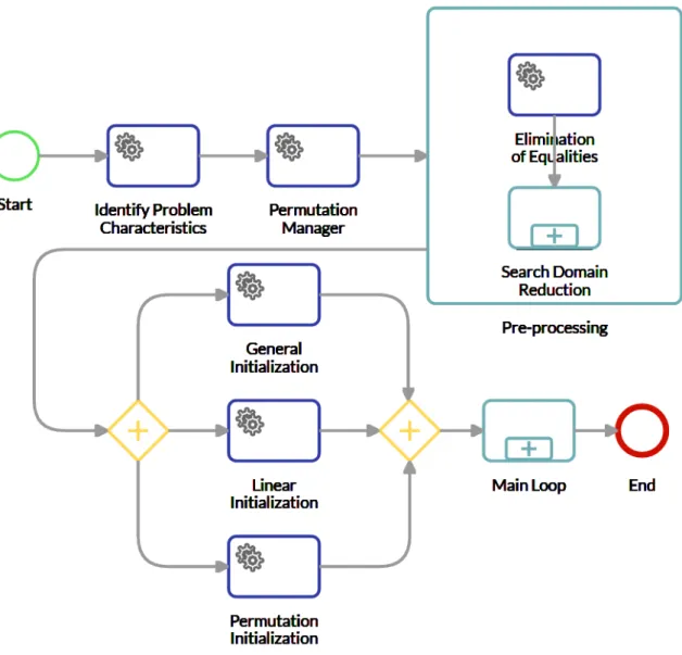
3.3 Initialization phase . . . 58
3.3.1 Identification of problem characteristics . . . 58
3.3.2 Permutation Manager . . . 59
3.3.3 Pre-processing . . . 59
3.3.4 General, linear and permutation initialization . . . 62
3.4 Solution Generation: Genetic Operators . . . 63
3.5 Double Population Mechanism . . . 65
3.5.1 Search Population management . . . 65
3.5.2 Update Reference Population . . . 65
3.6 Repair Phase . . . 67 3.7 Multi-Objective Approach . . . 67 3.7.1 Application to Single-Objective . . . 71 3.8 Termination Criteria . . . 71 3.9 Parameter Summary . . . 72 3.10 Mathematical Benchmarks . . . 73 3.10.1 Performance Metrics . . . 75
3.10.2 Single-Objective Optimization: Michalewicz Benchmarks . . . 82
3.10.3 Multi-Objective Optimization: Deb Benchmarks . . . 95
3.10.4 Benchmarks Outcome . . . 107
4 Bi-level Pricing Problems 111 4.1 Bi-level Programming: An Overview . . . 111
4.2 Metaheuristics for Bi-level Optimization Problems . . . 114
4.2.1 Evolutionary Algorithm for BOPs . . . 115
4.3 Metaheuristic Strategies for BOPs . . . 117
4.3.1 Single-level transformation approach . . . 118
4.3.2 Transformation to MOP approach . . . 119
4.3.4 Co-evolutionary approach . . . 120
4.4 Pricing Problem Applications: an Overview . . . 121
4.4.1 The bilinear pricing problem . . . 126
4.5 MOGASI: Framework Extension . . . 127
5 Network Pricing Problem 131 5.1 NPP on a General Transportation Network . . . 131
5.1.1 Arc pricing . . . 132
5.2 Path pricing . . . 133
5.2.1 Path Pricing vs. Arc Pricing . . . 134
5.3 Complexity of the Network Pricing Problem . . . 135
5.4 Bi-level Programming Formulation . . . 136
5.5 Highway Problem: NPP with Connected Toll Arcs . . . 137
5.6 One level Reformulation . . . 139
5.6.1 Valid inequalities . . . 140
5.7 MOGASI: Framework Application to NPP . . . 141
5.8 Experimental Design . . . 142
5.8.1 Instance Design . . . 143
5.8.2 Optimization Problem Setup . . . 143
5.8.3 Algorithm Parameter Tuning: Irace Package . . . 145
5.8.4 Initial Solution Creation . . . 145
5.9 Experimental Results . . . 146
5.9.1 Analysis of Complete Network Results . . . 147
5.9.2 Analysis of Partial Network Results . . . 152
5.9.3 Execution Time Analysis . . . 155
5.9.4 Time To Target Experiments . . . 158
6 Central Peak Load Pricing Problem 161 6.1 Air Navigation Service Charges . . . 164
6.2 Air Traffic - Current Situation and Growth Forecasts . . . 167
6.3 Pricing in Network-based industries . . . 170
6.4 Applicability of other pricing schemes to European ATM . . . 171
6.5 Route charge modulation in literature . . . 175
6.6 Centralized Peak Load Pricing . . . 176
6.7 Centralized Peak-Load Pricing (cPLP) model . . . 179
6.7.2 Model notation . . . 181
6.7.3 Central Planner (CP) problem, upper level problem . . . 182
6.7.4 Airspace Users’ (AUs) problem, lower-level problem . . . 185
6.7.5 Model formulation: bi-level cPLP . . . 187
6.7.6 Pricing schemes for cPLP . . . 188
6.8 MOGASI: Framework application to cPLP . . . 190
6.8.1 Instance Design . . . 192
6.9 Optimization Problem Setup . . . 198
6.9.1 Custom Solver Iteration . . . 199
6.9.2 Baseline Creation . . . 201
6.10 Experimental Results . . . 201
6.10.1 General Analysis . . . 201
6.10.2 Pareto Inspection . . . 204
6.10.3 Achieved Rate Modulation . . . 206
6.10.4 Achieved Traffic Redistribution . . . 209
6.10.5 cPLP application outcome . . . 210
7 Conclusions and Future Work 213
TABLE Page
3.1 Volume reduction by pre-processing on constrained problem . . . 62
3.2 Single-Objective Problem: NSGA-II parameters . . . 82
3.3 Single-Objective Problem: MOGA-II parameters . . . 83
3.4 Single-Objective Problem: MOGASI parameters . . . 83
3.5 Multi-Objective Problem: NSGA-II parameters . . . 95
3.6 Multi-Objective Problem: MOGA-II parameters . . . 95
3.7 Multi-Objective Problem: MOGASI parameters . . . 96
3.8 Final IGD values on the SCH problem . . . 97
3.9 Final IGD values on the KUR problem . . . 98
3.10 Final IGD values on the Deb problem . . . 100
3.11 Final IGD values on the SRN problem . . . 101
3.12 Final IGD values on the TNK problem . . . 102
3.13 Final IGD values on the OSY problem . . . 105
3.14 Final IGD values on the WATER problem . . . 106
4.1 Stackelberg vs Nash example: payoff matrix (Violin, 2014) . . . 113
5.1 Complete NPP Instances: Average Gaps and Execution Times . . . 148
5.2 Partial NPP Instances: Average Gaps and Execution Times . . . 152
5.3 TTT: Average Hits on total Tries in 180-commodity instances . . . 160
6.1 Largest airlines in Europe by total passengers carried in millions . . . 164
6.2 Current configuration of the route charges system (Rigonat, 2016) . . . 172
6.3 Centralized control with modulated charges configuration (Rigonat, 2016) . . . 173
6.4 Example of aircraft clustering results . . . 194
6.5 Cost scenario assigned to flights . . . 195
6.7 cPLP problem: MOGASI parameters . . . 202
6.8 cPLP - Baseline and selected best solutions . . . 204
6.9 Number of flights using different routes between two solutions . . . 209
FIGURE Page
2.1 Generic Genetic Algorithm Workflow . . . 7
2.2 Representation of a Chromosome . . . 8
2.3 Example of an application of single-point Crossover . . . 14
2.4 Application of multi-point Crossover with two cut points . . . 14
2.5 Possible problems in the adoption of a Genetic Algorithm . . . 26
2.6 Example of Genotype, Phenotype and Objective Space Relationships . . . 36
2.7 Plot of example functionF2(x) . . . 41
2.8 Implied Fitness Landscape for random populationP1 . . . 42
2.9 Implied Fitness Landscape for random populationP2 . . . 42
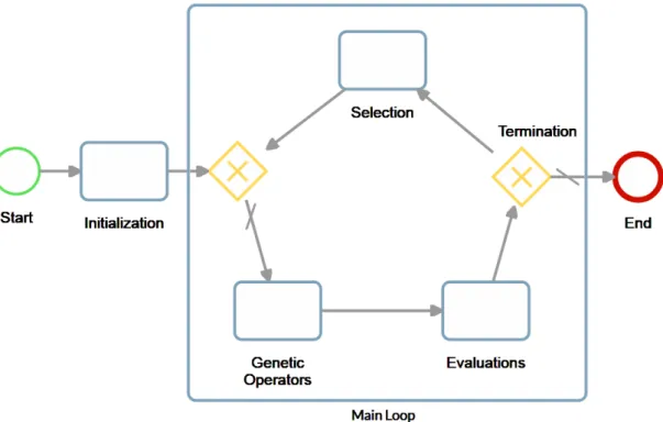
3.1 Graphical representation of a GA Main Loop with its generic phases . . . 55
3.2 Detailed initialization phase before the MOGASI optimization main loop . . . . 56
3.3 Simplified diagram of the MOGASI main loop . . . 58
3.4 Space reduction phases . . . 61
3.5 Representation of a single iteration of the standalone point generator . . . 66
3.6 Graphical representation of the Pareto Dominance concept (Santiago et al., 2014) 68 3.7 Empirical Attainment Function for Single-Objective (EAF-SO) . . . 76
3.8 Vertical Cut explanation on EAF-SO . . . 77
3.9 Horizontal Cut explanation on EAF-SO . . . 78
3.10 Additional considerations on the constrained problem on EAF-SO . . . 79
3.11 EAF comparison of two algorithms: darkest areas indicates a better performance of the plotted algorithm . . . 80
3.12 T01 problem: MOGASI vs MOGA-II . . . 84
3.13 T01 problem: MOGASI vs NSGA-II . . . 85
3.14 T02 problem: MOGASI vs MOGA-II . . . 86
3.16 T06 problem: MOGASI vs MOGA-II . . . 87
3.17 T06 problem: MOGASI vs NSGA-II . . . 88
3.18 T12 problem: MOGASI vs MOGA-II . . . 89
3.19 T12 problem: MOGASI vs NSGA-II . . . 90
3.20 T13 problem: MOGASI vs MOGA-II . . . 91
3.21 T13 problem: MOGASI vs NSGA-II . . . 91
3.22 T17 problem: MOGASI vs MOGA-II . . . 92
3.23 T17 problem: MOGASI vs NSGA-II . . . 93
3.24 T26 problem: MOGASI vs MOGA-II . . . 94
3.25 T26 problem: MOGASI vs NSGA-II . . . 94
3.26 SCH Problem: Performance Comparison . . . 98
3.27 KUR Problem: Performance Comparison . . . 99
3.28 DEB Problem: Performance Comparison . . . 100
3.29 SRN Problem: Performance Comparison . . . 102
3.30 TNK Problem: Performance Comparison . . . 103
3.31 OSY Problem: Performance Comparison . . . 105
3.32 WATER Problem: Performance Comparison . . . 108
4.1 Classification of metaheuristic strategies for Bi-level Optimization . . . 118
4.2 Metaheuristics nested repairing approach for solving BOPs . . . 121
4.3 Graphical example of the objective functions of the (bi)linear pricing problem in a two-dimensional case (Labbé et al., 1998) . . . 127
5.1 Simple example of an NPP (Dewez et al., 2008) . . . 132
5.2 Example of arc vs path pricing on a network with connected toll arcs . . . 135
5.3 Complete toll NPP (Heilporn et al., 2010b) . . . 138
5.4 MOGASI nested approach for solving NPP bi-level optimization problems . . . . 142
5.5 Complete NPP Randomly Generated Instances: Toll Perspective . . . 149
5.6 Complete NPP Randomly Generated Instances: Commodity Perspective . . . 151
5.7 Partial NPP Randomly Generated Instances: Toll Perspective . . . 154
5.8 Partial NPP Randomly Generated Instances: Commodity Perspective . . . 156
5.9 Execution times on 180-commodity partial instances . . . 157
5.10 TTT: Execution times analysis on 180-commodity partial instances . . . 159
6.1 ECAC member states (source: Eurocontrol) . . . 162
6.3 Average en-route ATFM delay per flight in the Eurocontrol area between 2006
and 2015 (source: Eurocontrol) . . . 168
6.4 SATURN mechanisms and the time-line of their application (SATURN D.6.5) . . 177
6.5 Example of an iterative decision loop for the cPLP optimization . . . 191
6.6 MOGASI nested approach for solving cPLP bi-level optimization problem . . . . 200
6.7 cPLP - Analysis of feasible solutions on the Parallel Coordinates chart . . . 203
6.8 cPLP - Alternative Pareto for Cumulative Capacity Violation vs Total Shift . . . . 205
6.9 Trade-offs among four Pareto solutions and the baseline solution . . . 206
6.10 Peak and off-peak rates for a selected ANSPs subset . . . 207
6.11 Peak and off-peak rates for Country12 (C12) . . . 208
C
H A P1
I
NTRODUCTION
B
i-level Programming Problems (BPPs) are hierarchical optimization problems where the optimal solution of the bottom level constitutes part of the top level constraints. A BPP can be viewed as a static version of the non-cooperative two-player game introduced by Stackelberg in the unbalanced economic market context. The first player, or leader, starts first trying to achieve his/her objective and to anticipate the possible responses of the second player, or follower. The follower also tries to achieve his/her objective and reacts to the leader’s actions but without considering the consequences of his/her actions on the leader’s objective. The choices available to both players are independent, so the leader’s decision affects both the follower’s objective and actions, and vice versa.BPPs are challenging and are well-known and studied in literature, but they are also becoming more and more relevant in the industrial sector. In fact, many real-world problems in areas such as management, economic planning or engineering involve a hierarchical rela-tionship between two decision levels. This poses several challenges, including randomness, two-level decision making, conflicting objectives and difficulties in searching for optimal solutions. Given the difficulties associated with solving BPPs, this field still lacks efficient solution methods. The issues connected to bi-level programming arise primarily from the nested structure of the problem. In recent decades there have been numerous attempts to develop dedicated algorithms, but most of the available methods can either only be applied to highly restricted classes of problems or are too computationally expensive, rendering them practically unfeasible in large-scale bi-level problems. For instance, the application of exact methods is generally unaffordable for very complex and large scale applications. As a
result, the tendency is to use specifically developed approximation algorithms with the aim of obtaining high-quality solutions in a reasonable amount of time that are hopefully closer to the optimal solution. Of these approximation algorithms, most promising is the family of heuristic and meta-heuristic algorithms.
Evolutionary heuristics have been used rather successfully to handle mathematical pro-gramming problems and applications that do not adhere to regularities such as continuity, differentiability or convexities. Owing to these characteristics, attempts have been made to solve Bi-level Optimization Problems (BOPs) using evolutionary heuristics since even simple (linear or quadratic) BOPs are intrinsically non-convex, non-differentiable and, at times, disconnected. More specifically, evolutionary algorithms for bi-level optimization were first proposed back in the 1990s. One of the first evolutionary algorithms for handling BOPs used a nested strategy, where the lower-level is handled with a linear programming method and the upper-level is solved with a Genetic Algorithm (GA). Nested strategies are indeed a popular approach for handling bi-level problems because for every upper-level decision variable configuration, a lower-level optimization task can be executed.
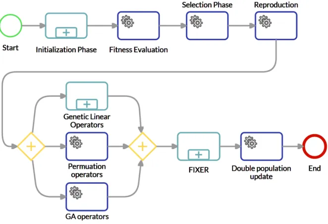
GAs, a class of evolutionary algorithms, are considered to be amongst the most effi-cient numerical strategies available because they are highly modular and easily adaptable to specific problems. They are particularly well-suited for complex non-linear problems or problems with multiple objectives which generate a set of Pareto optimal alternatives. Most of the GA bi-level techniques use the nested approach in which an outer algorithm handles the upper-level optimization task and an inner algorithm handles the lower-level optimization task, thereby making the overall bi-level optimization computationally very intensive. This work presents the Multi-Objective Genetic Algorithm for Structured Inputs (MOGASI). This algorithm combines modules and operators of standard GAs with special-ized routines aimed at achieving enhanced performance on specific types of problems. MOGASI classifies variables and constraints by applying specialized data handling strategies to sub-problems with different data structures. The algorithm has a classic pre-processing phase which restricts the feasible domain and reduces problem complexity by eliminating equality constraints. Unlike conventional GAs which work with a single population and evolve it towards optimal solutions, MOGASI works with two separate, concurrently existing but communicating populations. MOGASI also has a mechanism for replacing, whenever possible, unfeasible individuals. This algorithm has been extensively tested against a set of benchmarks well-known in literature and compared to other state-of-the-art GAs. Fur-thermore, it has been efficiently adapted to handle bi-level problems through a nested approach. In short, the GA is used at the upper-level and a custom solver at lower-level. This
The first application scenario is the Network Pricing Problem (NPP). It consists in a company needing to determine the price of its products/services so as to maximize its revenue or profit. At the same time, it must consider the customers’ reactions to these prices as they may refuse to buy a product or service if the price is too high. This class of problems was first studied in the 1990s and is NP-hard, although there are polynomial algorithms applicable to particular cases. The NPP application of the MOGASI algorithm concerns pricing problems in a road network, where typically an authority owns a subset of toll arcs and imposes tolls on them in an attempt to maximize revenues, whereas users traveling on the network seek to minimize costs. The NPP case described in the dedicated chapter involves connecting toll arcs to create a single path, similar to those used on highways. If users who leave the highway do not re-enter it, tolls can be simply imposed on paths uniquely determined by their entry and exit points. A custom set of instances was generated to analyze the possible differences between a solution with an exact solver and with an evolutionary bi-level approach. The main focus was on the behavior of the two approaches in relation to the increasing problem size.
The second application is the Peak-load pricing (PLP) problem, a two-tariff charging scheme commonly used in public transport and utilities. It is tested on the European Air Traffic Management (ATM) system as a means for redistributing air traffic and thus reducing airspace congestion in Europe. In particular, this work presents a centralized approach to PLP (cPLP) which presumes the existence of a Central Planner (CP) setting en-route charges for the entire network, as opposed in current system where charges are set in a decentralized way. CPLP consists in two phases. In the first phase, congested airspace sectors and their peak and off-peak hours are identified whereas in the second phase the CP assesses and defines en-route charges based on those hours in order to reduce the overall schedule displacement on the network. These charges should guarantee Air Navigation Service Providers (ANSPs) to recover their operational costs while inducing the Airspace Users (AUs) to route their aircrafts in a way that the network is able to sustain. The cPLP approach and the analysis presented in this work were developed in the framework of the SESAR WP-E project SATURN (Strategic Allocation of Traffic Using Redistribution in the Network), which investigated the possibility of mitigating the existing demand-capacity imbalances at the strategic level of flight planning, that is, months in advance of the day of operations, through the modulation of en-route charges. The solution of cPLP was tackled with a nested approach using MOGASI as the outer algorithm and a custom solver that was
specifically developed for the problem as the inner algorithm. The target was to show that significant improvements in traffic distribution in terms of both schedule displacement and air space sector load can be achieved through this simple en-route charges modulation scheme in a multi-objective implementation of cPLP. This approach solved much larger data instances than ever before, up to one day of traffic on the whole European network (ca. 30,000 flights over forty states).
To conclude, the innovative contributions stemming from the applications of the MO-GASI algorithm in a bi-level multi-objective optimization framework are summarized, jointly with the remaining open issues and the possibilities for future work.
C
H A P2
G
ENETIC
A
LGORITHMS
G
enetic algorithms (GAs) are an important type of meta-heuristics that are used to address hard optimization problems (De Jong and Spears, 1989). They are inspired by the Darwin’s evolutionist theory on the origin of species and natural selection. GAs belong to the larger class of Evolutionary Algorithms (EAs), the idea of which was introduced by Rechenberg (1965) and further developed in the following decades. The father of the GAs, due to his considerable contribution in the field, is deemed to be Holland (1975) of the University of Michigan.The functioning of GAs can be explained by considering the analogy with nature. When the individuals reproduce, their genomes, i.e. their chromosomes, are combined, so their offspring inherits some of the characteristics of each of the parents. Only the specimens with the best combination of genes are well adapted to a given environment and have the possibility to survive and create offspring. Such individuals are deemeddominating, whereas all others with genes ill-adapted to the environment are calleddominatedand are expected to eventually die out. Considering that mostly "good" genes are passed on, the overall goodness of the entire group of individuals, calledpopulation, will gradually increase generation after generation and over time the population will steadily improve and eventually evolve.
This theory is based on the following concepts:
• Individuals in a population carry genes with a number of different traits; • Genes are inherited from parents to offspring in different combinations;
• Individuals with the most advantageous gene combinations have the best chances for survival and reproduction in a given environment (survival of the fittest).
The chromosome of an individual is the result of the recombination and mutation of parents’ genes. GAs are stochastic algorithms that use random processes in their search and are able to take large, potentially huge search spaces, looking for optimal solutions. Random draws are often used in the initial population generation, in the selection of parents’ solutions, in the mating of selected solutions, and in the mutation of solutions. GAs are based on the idea that the recombination of solutions (individuals) in a population can potentially find new and better solutions called offspring. Translated into mathematics, each solution found by a GA is made of a combination or a mutation of elements of all variables that were used to generate it. These value combinations can be considered as the chromosome of the individual, whereas the values in each element constitute the individual genes.
Based on the problem characteristics (or environment in Natural Sciences), the algorithm computes a quantitative measure of goodness of a solution, referred to asfitness(adequacy to the environment). A selection of solutions with the highest fitness scores are preferred for the creation of subsequent solutions that have a higher probability to inherit good characteristics entailing higher fitness values. In the analogy with Natural Science the children generated by parents well adapted to the environment have a high probability to be well adapted too. Other, less fit individuals are discarded: the algorithm promotes the most promising portions of the problem space that should be searched intensively, keeping solutions residing there. In fact, it uses the survival-of-the-fittest principle to determine the individuals that will survive in order to become part of the new generation.
The steps of a GA can be summarized as shown in Figure 2.1. For a complete description of GAs’ structure and properties see Chapter 3 of Eiben and Smith (2003).
In GAs a fundamental concept is thediversityof solutions, which allows the algorithm to explore vaster areas of the search space. There are a number of factors explored and studied in literature that can influence diversity, starting from the different operators to preser-vation and propagation mechanisms. The initial population generation, parent selection, recombination operator, mutation operator, survivor selection, population size and repair operator can all affect a search profile and therefore diversity, as can the parameters used to implement each of these strategies. However, understanding and predicting the exact impact of a GA strategy on the search space and diversity is difficult because it implies that the true nature of the problem is known. If this were the case the most appropriate methods could be chosen to search it, but this knowledge would also make the use of optimization
superfluous. A clear example are engineering design optimization problems tackled in the industrial sector with the so-calledBlack Box Optimization(Muñoz et al., 2015), where the relationships between decision variables, objectives and constraints of the optimization problem are overly complex for a mathematical or analytic formulation. In this context, specialized engineering simulation solvers (e.g. thermodynamic simulations, finite element method simulations, and so forth) are used. Due to their intricate complexity it is almost impossible to make unique assumptions to fit a single optimization strategy. For this reason the GAs are particularly appreciated because of their stochastic nature (Michalewicz and Fogel, 2000; Turco and Kavka, 2011). In fact, they introduce a certain degree of randomness in the search process making the search less sensitive to modeling errors and escaping any local optima to converge to the global optimum without making additional assumptions about the underlying fitness landscape. It is therefore important to analyze how different GAs and methods implemented therein handle and maintain diversity and thus shape the search space.
2.1 Fundamental Genetic Algorithm Concepts
Mathematical and real-world problems have to be translated in a language that GAs are able to understand in order to solve them. Early GA research encoded individuals into a set of
binary stringsrepresenting each decision variable (Eiben and Smith, 2003), i.e. using sets of 1s and 0s. To perform an optimization of two real valued decision variables, a binary string would be generated for each of the two decision variables. Since early works on GAs used binary encoding, problem details were frequently not embedded in the GA. Even though modern GAs use a wide variety of encodings, many of them are not binary strings and the chosen operators are typically specific to the encoding of the solution and the problem details (Eiben and Smith, 2003). For the sake of clarity and simplicity the explanation of the fundamental GA concepts in the following paragraphs is based on the binary representation. The encoded representation of an individual is itschromosome. The genes of an individual are the decision variables and their components, i.e. the individual 1s and 0s, are thealleles. For example, assuming a model with two decision variables, x and y, and a solution encoded as 10010010, the first four alleles (or bits) 1001 form the individual’s gene representing a value of the variable x, whereas the last four alleles 0010 form the second gene of the individual’s representing a values of the variable y. 10010010 is thus the chromosome of this individual.
Figure 2.2: Representation of a Chromosome
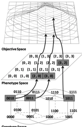
The individual's encoding, i.e. how it is represented so it could be understood and manipulated by a computing system, is itsgenotype. On the other hand, the same individual in the real world solution space is represented differently, that is itsphenotype. Depending on encoding, a given genotype may or may not represent all solutions that fully cover the
phenotype space, which is a well known issue discussed in literature (Michalewicz and Fogel, 2000). e.g. in the above example the phenotype space would contain all possible values of the variables x and y, whereas the genotype is the actual binary encoding of those values.
In a single-objective optimization framework each solution has a value for each objective, which determines its performance, i.e.fitness, with respect to that objective. The fitness values of all possible solutions make up thefitness space. An objective value of an individual is taken into account for the computation of its fitness, but it does not necessarily correspond to thefitness valuewhich determines the goodness of a solution. In fact, objective values can be artificially modified for different purposes, such as constraint handling and promotion of diversity.
Thefitness spaceshould not be confused with theproblem landscape, which is rather a mapping of the decision variables to the fitness space. The problem landscape term derives from its resemblance to a natural landscape with peaks and valleys, broad flat areas, areas of gradual increase or decrease and plateaus. Even though the majority of problems is multi-dimensional and cannot be so easily visually analyzed, the problem landscape concept is helpful for understanding other important GA concepts such asneighborhoods,exploration
andexploitation. The definition ofneighborhoodsin particular heavily shapes the definition of diversity of GA, but it is problem-dependent. Neighborhoods can be defined in many different ways (Michalewicz and Fogel, 2000); for instance, as a set of distances in the search landscape (phenotypic or genotypic) or as a set of distances in terms of objective values. Friedrich et al. (2007) compared these two metrics and concluded that both have impacts on runtime performance. Most diversity literature focuses on diversity measured in the phenotypic search space, which is likely due to natural definitions for distance in that space and our intuitive perception of the search space as a landscape.
2.1.1 Exploration and Exploitation Balance
Exploration/Exploitation Balance (EEB) is the degree to which the GA searches in areas far from current solutions or close to current solutions (Maturana and Saubion, 2008). In particular, exploration can be viewed as a global algorithmic search able to cover most of the search space, no matter how roughly, even far from current solutions, for the purpose of dis-covery of new individuals. It can thus help maintain GA diversity by including very different solutions in the search. Exploitation can be viewed as a local search around a given solution or set of solutions in limited portions of the search space. Exploitation generally quickens convergence as it produces solutions that are rather alike existing solutions, pressuring the population towards homogeneity by quickly replacing and driving out worse solutions. In
most GAs exploration and exploitation are performed concurrently so it is important to strike a balance in the search profile to match the specific problem characteristics and han-dle a possibly limited amount of available time and computational resources. For instance, too much exploration can easily turn into a completely random search and the algorithm may (or may not) stumble upon the best individuals by pure chance. On the other hand, too much exploitation will focus the search in areas that may not be the actual best areas of the problem landscape and leave others unexplored being too initialization point dependent. The crossover genetic operator, explained in section 2.1.4.1, can create solutions that are either close to parents (exploitation) or solutions that are farther from parents (exploration). Varying the degree to which the GA produces similar offspring can help manage diversity in the search process.
The concepts of exploration and exploitation are also closely connected to the definition of neighborhood in a problem landscape. When a new search point is within an already identified neighborhood, the algorithm is exploiting (solutions). If the new search point is outside the known neighborhoods, the algorithm is exploring. Since most GAs do not keep a history of visited places (Michalewicz and Fogel, 2000), exploration is often conveyed as a direct function of the current population rather than a function of all the visited places.
Convergence and diversity are directly related. The faster a GA converges, the faster diversity leaves the population. EEB is one of diversity management strategies that can be used to slow down convergence and thus reduce the impact of performance-degrading phenomena discussed in the dedicated subsection 2.2.
Focusing entirely on aspects of exploration and exploitation can be misleading (Eiben and Schippers, 1998). This is due to two factors: the EEB focuses on only a crisp definition of neighborhoods. Many definitions of exploitation and exploration are possible due to the ambiguous definition of neighborhoods. Focusing on the optimization of a single EEB can be misleading since many definitions of a neighborhood imply that there are more than one possible EEB to a problem. In general a good practice should be to dynamically adjust the EEB ratio during the run so that the first optimization steps have a higher exploration degree and that the final optimization steps have a higher exploitation degree. This can help the algorithm to collect sufficient information on the search space before focusing only on the refinement of the most promising areas.
2.1.2 The Schema Theorem
The Schema Theorem, developed by John Holland and first published in his book Adaptation in Natural and Artificial Systems in 1975 (Holland, 1975), is a milestone in GA theory as it
explains why GAs work so well in practice.
According to the Schema Theorem, GAs are a method that samples large portions of the problem space calledhyperplanes. Hyperplanes are nothing more than subsets of the entire set of solutions. Eachschemadescribes one such hyperplane containing all possible individuals for which all the genes match that schema. In other words it is a kind of a template that enables the exploration of similarities among chromosomes. In fact, some portions of a schema are defined, while others are not, which ultimately determines the differences between the members of the set. For example, using the binary representation, a schema could be the following: *11*0***, where 1s and 0s are fixed allele values, meaning that all individuals in this set contain exactly those values in the given loci, i.e. "1" in the second and third allele and 0 in the fifth allele. "*" symbols, on the other hand, arewild-cards, meaning that at least one solution in the set has a different value than all the others in that allele, either 0 or 1. No information on whether more individuals have one value or the other is provided. The number of fixed-values alleles (non "*") determines theorder of the schema. The above example is thus a 3-order schema. The distance between the first and the last fixed allele is calleddefining length. In the above example the distance is 3.
The Schema Theorem states that GAs perform well because short, low-order schemata with higher fitness increase exponentially in successive generations as a result of the applica-tion of the GA operators and the selecapplica-tion of the fittest individuals. It affirms that GAs sample hyperplanes (schema) in proportion to the representation of that schema in the population and the average fitness of the solutions sampled in that schema (Goldberg, 1989c).
More specifically, recombination and mutation genetic operators (discussed in Section 2.1.4) can be disruptive with regards to schemata. In general, the greater the defining length of a schema, the greater the probability that it is broken due to the crossover cut effect. Similarly, higher-order schemata have a greater probability of being broken by mutation than lower-order schemata. Finally, using a selection technique which chooses parents based on their fitness, fitter schemata will have a greater probability of finding their way unbroken from one generation to the next and also increasing their presence in the population.
Another fundamental concept closely related to the Schema theorem is the so called
implicit parallelismintroduced by Holland. It refers to the fact that the effective number of processed schemata is greater than the number of the processed structures, i.e. greater than the population size. More specifically, a population of size n with the chromosomes of lengthmcan contain up to 2m andn·2m schemata, but actually at leastn3schemata are processed without any extra memory or processing requirements. This is accomplished by continuously exploiting the currently available incomplete information on those schemata
while trying to find more information on them and other, possibly fitter schemata.
The Schema Theorem, however, has several shortcomings. Firstly, it considers only the disruptive effect of the genetic operators - it does not take into account schemata being constructed in this way. This phenomenon is explained by the Exact Schema Theorem (Stephens and Waelbroeck, 1996). Secondly, it focuses on the number of surviving schemata and not on which schemata survive. Such considerations have been addressed with the use of Markov chains, as illustrated in Nix and Vose (1992). Finally, the statement of an exponential increase of fit schemata, meaning that they are always fitter than the population average, is misleading (Goldberg, 1989c) because the average population fitness increases with time and converges with the fitness of the best schemata.
The Schema Theorem is proven only for a single generational change and hold only under the assumption of infinite population sizes. The populations for practical GA imple-mentations are always finite so any sampling error may lead to convergence of schemata in local optimum areas.
2.1.3 The Building Block Hypothesis
Matching the best partial solutions to construct better and better strings is the basis of the Building Block Hypothesis. It is closely related to the Schema Theorem because according to this hypothesis GA identifies and recombines short, low-order highly-fit schemata, called
building blocks, into increasingly fit individuals (Goldberg, 1989a). The emphasis in the GA is placed on the recombination of individuals rather than on mutation, as is the case with Evolution Strategies (Bäck, 1996).
Building blocks should thus be processed with the minimum disruption caused by crossover and mutation. For this purpose, an advance knowledge of the configuration of potential building blocks is important for the appropriate operator design, in particular crossover. The Building Block Hypothesis implies that for the GAs to be effective, solutions should have some complementary components (synergies to be combined into better solutions). Most traditional GA approaches to single optimization problems use overall fitness in survival and parent selection, instead of fitness based on the solutions component parts.
GA schema fitness definition is of paramount importance in this context, but its meaning is often unclear. Schema fitness can be interpreted as the average fitness of all individuals with that schema with respect to the average fitness of all individuals in the search space Sivanandam and Deepa (2008) call this version the "static building block hypothesis". Ac-cording to this interpretation, if all individuals but one in a schema have low fitness and the
one individual has very high fitness, the average fitness schema will be high, but nonetheless it is likely that this schema will disappear in a few generations. An opposite example is a schema containing many individuals with an above average fitness and few individuals with a very low fitness, resulting in a rather low average schema fitness. However, unlike the schema from the previous example, this schema will likely survive and produce good solutions. According to the abovementioned authors, a schema can be considered fit if the average fitness of its individuals in a number of population is higher than the average fitness of all individuals in all those populations. This interpretation is called the "relative building block hypothesis".
2.1.4 Standard Genetic Operators
Genetic operators are a core part of a GA because they guide the algorithm towards the solutions by promoting and preserving genetic diversity (mutation) and combining the existing solutions into new solutions (recombinationorcrossover). Mutation operates on a single chromosome so it is defined as the unary operator, whereas crossover operates on two chromosomes at a time and is thus defined as the binary operator.
2.1.4.1 Crossover
Crossover or recombination is the fundamental GA operator which takes more than one parent solution (chromosomes), combines their genes and produces one or more offspring solutions with the parents genetic material. Crossover can affect the algorithm convergence rate (i.e. the algorithm ability to find the optimal solution after as few evaluations as possible) because it can create individuals that are either very alike or very different from the parents. The dissimilitude of children to parents for different crossover operators is based partly on random choice, and partly on the crossover operator itself. The point of mating solutions is to transfer properties from differing parents in creating new offspring. According to the building block hypothesis, crossover attempts to create a child that is similar to the parents (probably located close to the parent genotype positions) but hopefully fitter than either of them. Selecting recombination operators that work in harmony with the overall GA strategy is important. Eiben and Smith (2003) provide more formal definitions for crossover and a good overview of a spectrum of crossover operators.
There are many recombination operators, most of which are problem specific. The fol-lowing are the most frequently used crossover types in GAs:
Thesingle-point crossovertakes the first part of one parent and splices it with the later part of a second parent. The point in which the crossover operator cuts between the two parents is determined by a random draw. If the random draw happens to be near the begin-ning or end of a solution, the created children will highly resemble one parent or another. Figure 2.3 below demonstrates how single-point crossover can generate two children with a 3rd position cut on a 8-bit gene representation. The chance of creating offspring that are identical or nearly identical to the parents using one point crossover depends on the number of alleles that the parents differ by in total and how identical the parents are in the first and last portions of their genotypic representation.
Figure 2.3: Example of an application of single-point Crossover
Goldberg (1989c) presents a generalized version of single point crossover called multi-point crossover. In this crossover the parent’s chromosomes are cut in multiple random points and the alternating segments are then swapped between the parents to create off-spring. The example on the figure below is a two-point crossover.
Figure 2.4: Application of multi-point Crossover with two cut points
Inuniform crossover(UX) the chromosome are not divided into segments, but each gene is rather treated differently. UX picks which genes will be inherited from the different parents based on individual random draws for each non-unique allele. UX selects on average half of the genes from one parent and half from the other. The likelihood that parents will generate identical offspring (to the parents) is a function of the number of different alleles between the parents. For a genotype represented as a string of binary digits the likelihood of generating exact replicates of the parents can be approximated by the binomial distribution
wherenis the number of bits differing between the parents,pis the probability of selecting a 0, and m is the exact number of successes to check. The binomial distribution is represented with the probability mass function as follows:
(2.1) P(M=m)= n!
m!·(n−m)!·p m
·(1−p)n−m
For the typical UX operator,p=0.5 which makes the distribution symmetric aboutn/2. For parents that produce exact copies of children,mmust be 0 orn. For instance, to calculate the probability that parents that differ by five bits will generate exact replicates,nis 5,pis 0.5, andmis 0 and 5. For this example, the probability of creating an exact copy of either parent is 6.25 percent. As n increases, there is a lower chance of obtaining an exact copy of either parent via UX.
Another example is thehalf uniform crossover(HUX) operator proposed by Eshelman (1991), which is a variation on the UX operator. The HUX ensures that exactly half of the bits that are different between parents convey from one parent and the other half convey from the second parent. This operator ensures maximum diversity of the produced offspring. A child will have equal properties of both parents but can never be an exact copy of a parent, except when the parents differ by no more than one bit. Mauldin (1984) proposed a crossover operator that checks the offspring against the current population after normal crossover. If the offspring differs by less thankbits from any member in the population, bits are flipped at random until the offspring differs at least bykbits from each member. This method has the potential to introduce significant amounts of new genetic material into the gene pool. Over timekis gradually reduced to focus the efforts on solutions that are closer together as the algorithm progresses, this could remember an annealing procedure. This approach was the first attempt by GA researchers to explicitly maintain diversity in the current population.
2.1.4.2 Mutation
In simple terms, the mutation operation may be defined as a small random alteration in the chromosomes of an individual to get a new solution. It is used to maintain and introduce diversity in the GA population. For this reason, mutation is primarily referred to as an exploration operator. Most mutation operators are purely random and thus very high mutation rates can force the GA to become no better than random search. Pure random non-repeating search is often not the best search strategy on a constrained budget as random search does not use known problem information or structure. Normally, mutation rates are kept low so that the GA heuristic can work. Variable mutation rates often give better
results than static mutation rates. GA search often benefits from an adaptive or self-adaptive approach controlling the mutation rate (Thierens, 2002).
Different kinds of mutation operators exist. For instance, in the bit flip mutation one or more random bits are selected and flipped. This is used for binary-encoded GAs. Random resetting is the extension of the bit flip mutation for integer representation: a random value from a set of allowed values is assigned to a randomly chosen gene. In swap mutation, random positions in a chromosome are selected and interchanged. Scramble mutation chooses a subset of genes from the entire chromosome and shuffles their values randomly. In inversion mutation a chosen subset of genes is not shuffled but instead the entire string is merely inverted. These last three types are commonly used in GAs to solve problems with order-based encoded solutions.
Unlike standard mutation, cataclysmic mutation or mass extinction (Eshelman, 1991) is a widespread changing of many alleles in multiple solutions or the killing-off of many solutions in a single phase of an algorithm. This type of mutation can generally be thought of as being a reset or restart of the search process.
2.1.5 Selection Pressure
Selection pressure can be defined as the level of selectivity of the GA, that is its tendency to select only the best individuals in the current generation, either as parents or for survival. On one hand, an excessive selection pressure can have a negative impact on the genetic diversity and thus lead the algorithm towards a local rather than the global optimum. On the other hand, insufficient selection pressure will slow down convergence (Goldberg and Deb, 1991). For these reasons most GAs avoid taking only and exclusively the fittest of the population for reproduction and discarding all others. Such a strategy maintains a higher genetic diversity in a population because even the less fit individuals have a chance to reproduce. This enables the algorithm to better explore the search space and possibly find excellent solutions in unexpected regions, instead of concentrating on a narrow area. The actual amount of selection pressure depends on the implemented method.
Parent selection determines which solutions will be subject to genetic operators to pass on their genetic material to the offspring. It has therefore a direct impact on crossover diver-sity and convergence rate, for example mating parents that are very similar generally results in more exploitation while mating parents that are very different results in more exploration. The most common parent selection operators are tournament selection, roulette wheel selection, rank-based selection and random selection, each entailing a different selection pressure. They are explained below:
• Thetournament selectionis generally intended as a competition between two or more random individuals: the fittest among them wins and becomes a parent. It usually involves generating a random value for each individual taking part in the competition and comparing it to a pre-determined selection probability. If the random number is less than or equal to the selection probability, the fitter solution is chosen; otherwise, the weaker solution is chosen. This probability is usually a parameter and it can be therefore used to adjust the selection pressure and thus influences the population diversity.
• Theroulette wheel selection(Holland, 1992) gives every individual a chance for being selected, even though this chance is greater for fitter candidates. Each individual is allocated a section of an imaginary roulette wheel of a different size proportional to their fitness, i.e. the fittest candidate has the largest slice, whether the weakest candidate has the smallest slice. After the wheel is spun the individual associated with the winning section is selected. The wheel spinning occurs as many times as is required to select the sufficient number of parents to produce the next generation. It may happen that particularly fit individuals are selected more than once as parents. For this kind of selection if fitness variance is low, it is more likely that parents will be selected from diverse parts of the population. Conversely, more variance in solution fitness indicates that there is a higher probability that the selected parents are fitter. Thus, in populations that have high fitness variance, roulette wheel selection is more likely to breed only the top individuals. This causes faster convergence than a roulette wheel selection on a population with low variance.
• Inrank-based selectionthe individuals are sorted according to their fitness and as-signed a selection probability proportional to their ranking regardless of the actual fitness score. This avoids premature convergence and stagnation in the same search re-gion(s) because it is not important if a solution is 100% or 1% fitter than the next: what matters is their ranking against other individuals. As the fitness differences among solutions decrease in the course of the search, the selection pressure increases. • Inrandom selectionindividuals are selected randomly from a population. This
opera-tor is beneficial for diversity, but not for convergence, and if used alone it may easily result in the loss of good candidates if the offspring is weaker than the parents. For this reason it is usually coupled with the elitism approach. Elitism consists in copying a small portion of the fittest individuals unchanged to the next generation increasing the probabilities that their traits are passed on as they are eligible for selection as
parents just like all other individuals in a generation, but may easily appear in several generations.
Another main type of selection is the so-calledsurvivor selection. It determines which individuals survive and become part of the next generation and which do not. For this reason it is sometimes referred to as population resizing method. It is crucial that it ensures that the fitter individuals are not lost, but at the same time without keeping those individuals only since this may lead to loss of diversity and premature convergence. Many GAs use elitism for this purpose. The simplest survivor selection strategy is randomly choosing the surviving individuals. This approach, however, can lead to convergence issues. Inage-based selection
(Eiben and Smith, 2015) the notion of fitness is not used. Instead, each individual exists in the population for the same number of iterations. In a generational model the number of offspring is the same as the number of parents so each individual exists for just one cycle and the parents are simply discarded. This does not preclude that genetic materials of some individual might persist over time in the population, but for this to happen the configuration must be replicated by the crossover or the mutation stages, as it was explained in subsection 2.1.4. An increase of the mean fitness over time relies on having sufficient parent selection pressure and using operators that are not too disruptive.
A wide number of fitness-based survivor selection strategies have been proposed in literature (Eiben and Smith, 2015). The idea is that the children replace a number of the least fit individuals in the population, usually based on a general ranking according to the Pareto domination criteria combined with some diversity management strategies (see Section 3.7). For example, in Whitley’s GENITOR algorithm (Whitley, 1989) a number of worst parents in the population is selected for replacement. Although this can lead to very rapid improvements in the mean population fitness, it can also lead to premature convergence as the population tends to rapidly focus on the currently present fittest member. For this reason, it is commonly used in conjunction with large populations and/or "no duplicated solutions" strategy. The elitism approach to survivor selection is often coupled with the age-based and stochastic fitness-based strategies to prevent the loss of the fittest members of the current population. In this way, one or more currently fittest members in the population is kept instead of being replaced by less fit offspring individuals.
Based on the survivor selection approach and on the evaluation mechanism, a GA can be generational or steady-state.Generational GAscreate individuals in batches: a new offspring set is created from the members of the current generation and the members of the next generation are selected among both parents and offspring.Steady-state GAsdo not have generations: instead, the selection process occurs as the individuals are created and, if
selected, the new individual is inserted in the new population at any time. In general, steady-state approaches have a higher survivor selection pressure than generational approaches, but in many cases they are preferred owing to their ability to efficiently exploit computational resources.
2.2 Performance Analysis
According to the Schema Theorem, the highly fit schemata can be found over time in an ex-ponentially increasing number of samples, resulting in narrower and narrower search areas (Mitchell et al., 1991). In other words, exploration predominates early on in a run of a GA, but over time the GA converges more and more rapidly to the fittest schema and exploitation becomes the dominant mechanism. The Schema Theorem is based on the assumption of infinite size populations, so in case of finite size populations, any, no matter how small, sampling error may be magnified and cause premature convergence (Goldberg, 1989c). It is a state of degeneration of the GA search where the population becomes dominated by one or more suboptimal solutions. According to literature (Mahfoud, 1995; Maturana and Saubion, 2008; Oppacher and Wineberg, 1999; Smith et al., 1993), premature convergence is one of the main issues that can degrade GA performance, beside other phenomena such asepistasis,deception,genetic drift,duplication,hitchhikingandoperator bias. Even the metric used for the survival selection can affect the convergence behavior of the algorithm in relation with the shape of the problem landscape.
These negative forces are better explained in the following sections.
2.2.1 Epistasis and Deception
In genetics, a gene is said to be epistatic to another gene if it masks the phenotypic expression of the second one (Strickberger, 1968). Rawlins (1991) introduced the analogous notion in the GA theory by defining the minimal epistasis as the situation in which every gene is independent of every other gene and the maximal epistasis as the situation in which no subset of genes is independent from any other.
Deception is a special case of epistasis (Beasley et al., 1993), which occurs when the selection pressure leads the GA search away from the optimal solutions, i.e. low-order schemata do not lead to optimal points but instead lead away from them, or towards sub-optimal points (Goldberg, 1989a,b).
Epistasis and deception are not entirely distinct since deceptive functions by definition must have some component interactions. They are essentially independent but can mutually reinforce each other. Epistasis does not necessarily entail low order schemata to lead away from the optimal solution: a problem where all solutions but one have sub-optimal values can still be difficult for a GA even without deception. In this case it might be that the low order schemata simply do not indicate a direction of increasing fitness. Problems that have the highest levels of epistasis do not contain regularities in the search space and as a result heuristics are no better (and often worse) than non-repeating random search. Grefenstette (1992) concluded that deception is not the only condition that makes a problem hard for GAs. Grefenstette (1992) also demonstrates that deception can be viewed as a dynamic phenomenon using an example that showed how a GA can be deceived (for a while) and still reliably find the optimal solution.
Even though it is a not a perfect solution, diversity management represents an efficient way to manually fight deception because in spite of undesired alleles surviving for a long time, it slows down convergence giving the GA time (and space) to stumble upon the good solution. In other words, GA with high diversity are less prone to be fooled by the phenomenon of deception.
Several authors (Goldberg, 1989a,b; Liepins and Voset, 1990; Whitley, 1991) have studied the properties of a particular class of epistatic problems, known as deceptive problems. However, for solving practical problems it might be more important to be able to estimate the degree of epistasis to shape the most suitable strategy for tackling the epistasis itself. For instance, Davidor (1991) shows that problems with very little epistasis are generally simple to solve. On the other hand, highly epistatic problems are unlikely to be solved by any systematic method, including the GA. The encoding used for a GA (Radcliffe, 1992; Vose and Liepins, 1991), i.e. the solution representation, is also of critical importance. In fact, the appropriate choice of encoding may reduce epistasis in a problem, just like an inappropriate encoding may increase it as much as to make a problem unsolvable for the GA.
Several methods of problem sampling have been proposed to date to determine the degree of epistasis in a problem through problem landscape analysis. Davidor’s measure of epistasis variance was the first attempt (Davidor, 1991) but the measure did not account for possible scaling in fitness and the number of negative and positive interactions (Reeves and Wright, 1995). Measures of normalized epistasis were proposed to address possible bias from scaling the magnitude of fitness values (Naudts et al., 1997; Vanhove and Verschoren, 1995). Reeves and Wright (1995) proposed aDesign of Experiments(DOE) approach using contrasts. This approach breaks the interactions into different groups that simulate a number of effects
together. The DOE approach is attractive because both magnitude of change and direction of change can be accounted for in the analysis. However, like all the other methods to date, the DOE approach requires assumptions about the significance of different interactions in order to provide a meaningful insight since effects must be aliased together in an incomplete sampling of the problem space. The problem of measures of epistasis based on problem space sampling is that if it was known what makes the problem hard, it could be isolated to make the problem easy. However, most GAs work on extremely large problems where a large-scale sampling of the space is time-prohibitive. Determination of when a problem is well suited for a GA is likely better done according to past experience with similar problems and any knowledge that can be gleaned from input data rather than from objective space sampling.
2.2.2 Genetic Drift
Genetic drift is the process of accumulating stochastic errors in the population gene pool resulting in a premature convergence to a sub-optimal solution. It is caused by random increases in the number of alleles of the same type forming genes over time. Once it begins, the genetic drift will continue until the involved allele is either lost or remains the only allele present at a particular locus. Eiben and Smith (2003) describe a simple example to demonstrate drift: a GA with the population of individuals evenly split in half between two solutions with equal fitness. Without considering the effects of mutation and crossover, the example shows how the population must converge to either solution due to drift error through an argument based on probability.
Even when there is a significant difference in fitness between the best solution and the population, there may be a fair probability that a converged population causes the algorithm to melt down the hill to sub-optimal solutions. As the population size gets larger and fitness values more similar, the force of drift can be even more significant. This phenomenon can be partially remedied by using an elitist survival strategy. However, drift effects can also happen on sub-elite solutions such that drift is not prevented simply by using an elitist strategy.
The population can be thought of as having properties of inertia where a converged population tends to stay in a converged state. Populations having properties of inertia that implies early influence on the search can be important as it gets more difficult to affect bias later in the search.
Genetic drift can be countered with diversity management techniques. Diversity in a population slows genetic drift rates because drift is partially a function of population similarity. It takes more steps for a GA to drift to a single solution if there is greater diversity
since one solution must force out all of the other solutions from the population to cause complete convergence. When the population members are similar, the GA may need to replicate only a few solutions to completely converge. Genetic drift typically occurs in smaller populations where some alleles are present in fewer copies and are more likely to be lost, whereas it takes more steps to cause convergence in a larger population because of a large gene pool. In any case the selection pressure should be greater than the drift pressure to prevent convergence to an arbitrary solution. Gibbs et al. (2008) proposed a way to calculate the population size for real-based problems to ensure that the selection pressure is greater than genetic drift given a set of assumptions and operators.
However, this method is highly restricted to the problem representation (real values) and associated operators. Much discussion has been given to genetic drift although little research has been done to characterize drift rates when combined with selection pressure in a GA. It is hard to distinguish which convergence in a particular run or set of runs is due to drift and which convergence is due to the selection pressure, making online measurement of drift rates difficult.
2.2.3 Duplication
Most GAs do not check that solutions are unique, resulting in a certain level of duplication of solutions in a population. Population convergence is the extreme case of duplication where every individual in the current population is identical or at least they share most of their genetic material. Duplication occurs less prior to convergence. Duplication can be harmful because it increases drift pressure and repeated function evaluations occur for copies of the same individual consuming additional computational resources. However, ensuring solution uniqueness in a GA is also costly because it requires a pairwise comparison of all individuals. Since the problem landscape is normally much larger than the number of sampled points, most GAs do not check for complete diversity of all individuals within a run. The rate of duplication of individuals for a GA is a function of the diversity properties of the GA, the population size and the proportion of sampled points compared to the solution landscape size. Large solution landscapes do not necessarily mean that solutions will not be repeated because the negative effects of drift, inappropriate selection pressure or landscape shape should also be accounted for. Although using large population sizes should usually reduce drift and selection pressure, and thus slow down convergence, this may not be feasible in case of limited computation resources. In fact, in such cases a trade-off is achieved by reducing the number of generations, which in turn does not give the GA the possibility to properly converge to the optimum.
2.2.4 Hitchhiking
Hitchhiking is another phenomenon that may lead a GA astray during its search. It has been defined so by Forrest and Mitchell (1993) in their attempt to show how GAs use building blocks to generate better solutions, even though it has been also previously discussed (under the name "spurious correlation") by Schraudolph and Belew (1992) and Eshelman (1991), among others.
Forrest and Mitchell (1993) created a problem set called the Royal Road where GAs were hypothesized to outperform hill climbers on a simple structured problem. The results were counter-intuitive to their hypothesis and showed that the GA performed significantly worse than the hill climber on the Royal Road problem. The article provided evidence that high fitness solutions (not optimal) quickly dominated the results of the runs despite the fact that parent selection pressures were reduced. The reason behind this underperformance was the phenomenon they called hitchhiking. Once a higher-order schema with high fitness is discovered, this schema spreads quickly through the population with sub-optimal alleles hitchhiking along with the ones in the schema’s defined positions. This slows down the discovery of schemata in other positions, especially those that are close to the highly fit schema’s defined positions. In this way hitchhiking seriously limits the implicit parallelism of the GA by restricting the schemata sampled in certain allele positions.
Fitter solutions got a higher chance of becoming parents so a reduction in parent selec-tion pressure led to less bias toward selecting parents with high fitness. This quick dominance of single solutions caused problems for the GA in constructing the overall optimal solution as diversity was driven out of the population. The single solution that dominated the pop-ulation carried with it a series of suboptimal bits, but because it was able to take over the population, the suboptimal bits associated with that solution also became dominating even though they did not contribute positively to the fitness of the solution.
Formally, hitchhiking is the process of poor alleles being represented in many individuals in a population because they are associated with a highly fit solution. No amount of hitch-hiking is useful, but some amount is unavoidable as, by definition, sub-optimal solutions must always contain a component part that is sub-optimal. Hitchhiking can be reduced with diversity management methods because when similar solutions are not allowed to reside in the population, hitchhiking is reduced.
2.2.5 Operator Bias
When selected parents are combined to create offspring, ideally GAs could determine the ’best’ traits to be passed on. However, this is rarely the actual case as there are a vast number of ways to combine two solutions. This has led to a large body of literature studying various recombination operators for different representations and problems. In GAs, recombina-tion is also commonly described as crossover, as already introduced in subsecrecombina-tion 2.1.4.1. Crossover operators are known to be biased toward selecting certain bits from different parents instead of others (Eshelman, 1991). On one hand, positional bias refers to how bits that are close together in the genotype of a given solution are likely to stay close together (Eiben and Smith, 2003). In single-point crossover the chromosomes of each parent are cut in one random location and the genes, i.e. variables, at each side of the cut are exchanged to form two new individuals. The first part of a child comes from one parent, whereas the second part comes from the other, and vice versa. The single-point crossover has therefore high positional bias. Moreover, the positions of the alleles have an effect on what solutions are created. Parents with the respective genotypes 0000 and 1111 in this case cannot produce a child with a genotype where 0s and 1s are interlaced because their bits come from single consecutive strings of each of the parents. Distributional bias, on the other hand, refers to the number of bits parents are expected to pass on to their children (Eshelman, 1991) and for example it is a characteristic of one of the classic genetic operators, the Uniform Crossover (UX). UX uses a mixing ratio which defines the number of genes passed by one parent and the other to their offspring and each bit of the parents'strings is evaluated for exchange with a fixed probability, which is typically 0.5. A larger number of bits that differ between the parents entails a lower probability that only a few bits from a parents are selected. For this reason in case of very different individuals UX searches farther away from them, i.e. per-forms more exploration than exploi