Real-Time Stream Processing in Embedded Systems

(1)

Real-Time Stream Processing

in Embedded Systems

Haitao Mei

Doctor of Philosophy

University of York

Computer Science

September 2017

(2)

(3)

Abstract

Modern real-time embedded systems often involve computational-intensive data processing algorithms to meet their application requirements. As a re-sult, there has been an increase in the use of multiprocessor platforms. The stream processing programming model aims to facilitate the construction of concurrent data processing programs to exploit the parallelism available on these architectures. However, most current stream processing frameworks or languages are not designed for use in real-time systems, let alone systems that might also have hard real-time control algorithms. This thesis contends that a generic architecture of a real-time stream processing infrastructure can be created to support predictable processing of both batched and live streaming data sources, and integrated with hard real-time control algorithms.

The thesis first reviews relevant stream processing techniques, and iden-tifies the open issues. Then a real-time stream processing task model, and an architecture for supporting that model is proposed. An approach to the integration of stream processing tasks into a real-time environment that also has hard real-time components is presented. Data is processed in parallel us-ing execution-time servers allocated to each core. An algorithm is presented for selecting the parameters of the servers that maximises their capacities (within an overall deadline) and ensures that hard real-time components re-main schedulable. Response-time analysis is derived to guarantee that the real-time requirements (deadlines for batched data processing, and latency for each data item for live data) for the stream processing activity are met. A framework, called SPRY, is implemented to support the proposed real-time stream processing architecture. The framework supports fully-partitioned ap-plications that are scheduled using fixed priority-based scheduling techniques. A case study based on a modified Generic Avionics Platform is given to demon-strate the overall approach. Finally, the evaluation shows that the presented approach provides a better schedulability than alternative approaches.

(4)

(5)

List of Figures

1.1 A stream processing example . . . 2

1.2 The mission of the generating images of target areas using SAR. 4 2.1 A stream processing example . . . 13

2.2 A pipeline that has 4 filters . . . 16

2.3 The evaluation of a pipeline. . . 16

2.4 A control-parallel pipeline. . . 18

2.5 A data-parallel pipeline. . . 19

2.6 The hybrid pipeline. . . 20

2.7 StreamIt SplitJoin example, the cycle with numbers represent the input data or an intermediate result. . . 24

2.8 Spark-Streaming-flow . . . 28

2.9 Structure of D-Streams . . . 29

2.10 Applying the flatMap operation on a D-Streams . . . 29

2.11 Spark DAG evalutation stages . . . 31

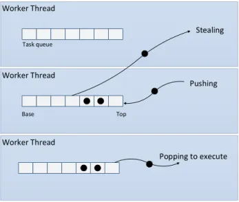
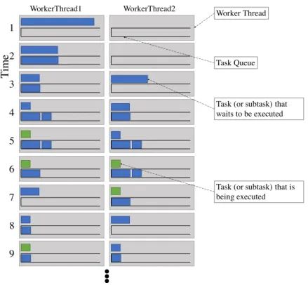
2.12 Tasks stealing, pushing and popping within worker threads . . 35

2.13 Java 8 stream parallel evaluation . . . 37

2.14 StormTopology . . . 39

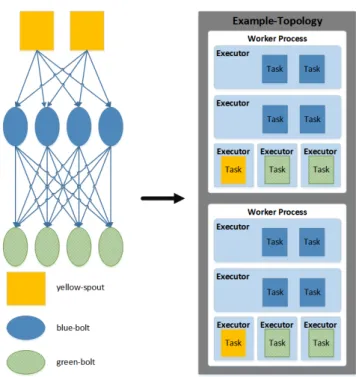
2.15 Storm topology mapping . . . 41

2.16 Inside of a node in Storm Cluster . . . 42

2.17 Work-stealing in a stream processing system with a pipeline . . 46

3.1 The pipeline software design pattern . . . 51

3.2 Stream processing from different data sources. . . 52

3.3 Real-time batched data processing overview . . . 53

3.4 Real-time data flow processing overview . . . 53

3.5 Real-time stream processing system overview . . . 54

(12)

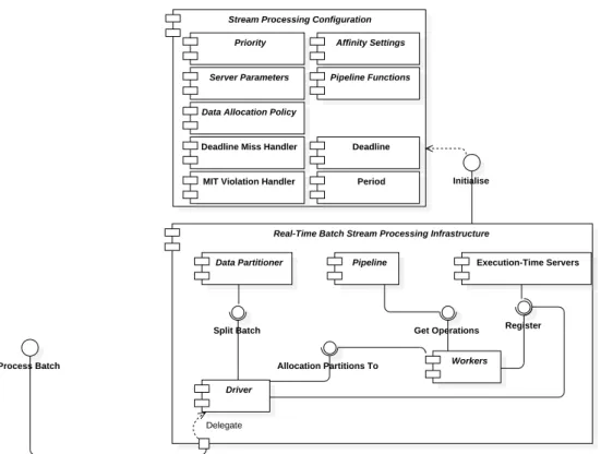
3.7 Real-time batched stream processing infrastructure component

diagram. . . 59

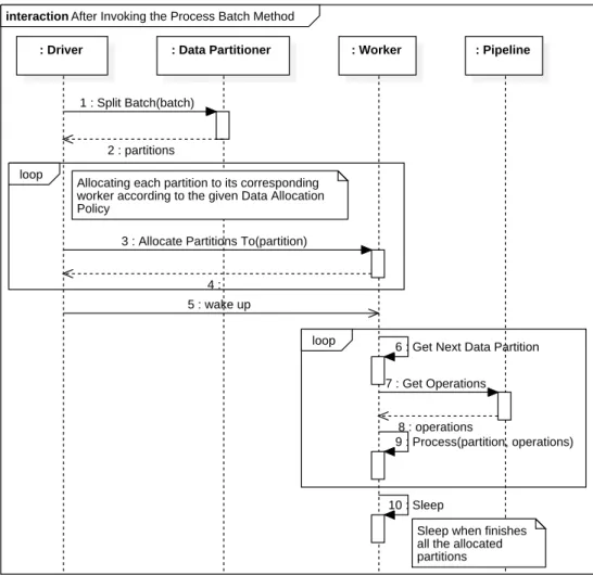
3.8 Batch Processing Procedure . . . 63

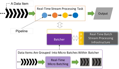
3.9 The Real-Time Streaming Architecture . . . 66

3.10 The real-time micro-batching state machine . . . 67

4.1 The structure of the stream processing task. . . 74

4.2 Data processing window within the stream processing task . . . 78

4.3 The latest time when the epilogue starts. . . 78

4.4 Server generation algorithm. . . 82

4.5 The subroutine used by the server generation algorithm. . . 83

4.6 Configuring the stream processing task. . . 86

5.1 Double hit . . . 93

5.2 The critical instance and busy period. . . 94

5.3 Stream RTA pessimism . . . 103

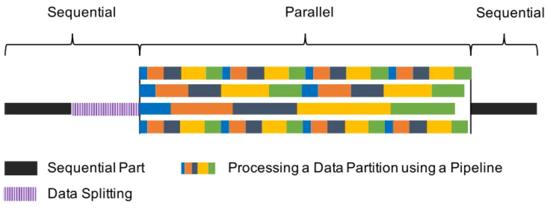
5.4 The worst-case execution of the stream processing. S represents the real-time stream processing task. . . 109

5.5 The mission of the generating images of target areas using SAR. 110 5.6 Illustration of a SAR operating on a target area, using the spot-light mode. . . 111

5.7 The worst-case execution of the stream processing. . . 116

6.1 SAR Stream Pipeline . . . 121

6.2 The observed worst-case response times of the SAR benchmark executing with different parallelism. . . 123

6.3 The percentage of the computation time required by each filter in the SAR benchmark. . . 124

6.4 StreamIt filter bank benchmark . . . 125

6.5 The observed worst-case response times of the filter bank bench-mark. . . 126

6.6 The implementation of SPRYEngine and corresponding com-ponents in the real-time stream processing architecture. . . 128

6.7 The implementation of Batched Streams and corresponding com-ponents in the architecture. . . 140

7.1 The maximum computation time can be provided by a single or multiple servers . . . 152

(13)

7.2 The accuracy of the presented analysis approach. . . 153 7.3 Compares SPRY with a traditional embedded approach for batched

data processing . . . 155 7.4 Compares SPRY with a traditional embedded approach with

overheads . . . 157 7.5 SPRY scalability evaluation . . . 158 7.6 The system’s schedulability with different live streaming data

sources. . . 160 7.7 The schedulability of the system for a live streaming processing

task with a MIT of 10 time units, WCET of processing each data item of 100 time units, latency of 1000 time units, with 128 hard real-time tasks. . . 161 7.8 The schedulability of the system for a live streaming processing

task with a MIT of 2 time units, WCET of processing each data item of 10 time units, latency of 30 time units, with 128 hard real-time tasks. . . 162 7.9 The schedulability of the system for a stream processing task

with a period of 15 time units, 16 data partitions (WCET of each is 10 time units), and the deadline of 10 time units. The system also has 128 hard real-time tasks. . . 163 7.10 The schedulability of the system for a stream processing task

with a period of 15 time units, 16 data partitions (WCET of each is 10 time units), and the deadline of 10 time units. The system also has 128 hard real-time tasks. Allocating servers before hard real-time tasks. . . 164

B.1 The accuracy of the presented analysis approach for the tradi-tional embedded approach. . . 187

(14)

(15)

List of Tables

2.1 Stream Processing Techniques Classification . . . 21

5.1 Real-time Tasks Characteristics . . . 104

5.2 Possible Deferrable Servers For ProcessorP0. DP W Represents the Data Processing Window. . . 105

5.3 Possible Deferrable Servers for Processor P1. DP W represents the Data Processing Window. . . 107

5.4 Selected Deferrable Servers . . . 108

5.5 Hard real-time tasks in the system. P roc is the assigned pro-cessor ID. . . 112

5.6 Possible Deferrable Servers For ProcessorP0. DP W Represents the Data Processing Window. . . 113

5.7 Generated Deferrable Servers . . . 113

5.8 Input Partitioning . . . 114

5.9 Worst-Case Latency of Image Generation. . . 117

6.1 Variations in the SAR Stream Processing Response Times. Co-efficient of Variation (CV) Represents the Standard Deviation/the Mean Response Time. . . 122

6.2 Variations in the Filter Bank Stream Processing Response Times. Coefficient of Variation (CV) Represents the Standard Devia-tion/the Mean Response Time. . . 126

A.1 The two-way ANOVA results for SAR Benchmarks. . . 181

(16)

(17)

Acknowledgement

Firstly, I would like to present my gratitude to my supervisors: Prof. Andy Wellings and Dr. Ian Gray, for their guidances and help during my whole study. I received a lot of help from them not only for the research, but also for my daily life so that the whole research procedure has been very rewarding.

I would also like to thank my family. Without the support from my parents, I would not be able to finish my Ph.D study. Their help allowed me to focus on the research, rather than also considering the living costs, etc.

I also acknowledge the Computer Science Department’s scholarship, with-out which I would not have been able to fund the Ph.D program.

I would also like to thank the members in the Real-time Systems group, they are so patient to explain the problems I had, and encouraged me to carry on my research.

Last but not least, I want to thank my friends, for their help for both study, and especially life. They helped me to pass each obstacle in daily life, and ease the pain.

(18)

(19)

Declaration

I declare that this thesis is a presentation of original work and I am the sole author. This work has not previously been presented for an award at this, or any other, University. All sources are acknowledged as References.

Parts of this thesis have previously been submitted or published in the following papers:

• H. Mei, I. Gray, and A. Wellings. Integrating Stream Processing into Embedded Real-Time Systems. Submitted to the Journal of Real-time Systems. Springer, 2017.

• H. Mei, I. Gray, and A. Wellings. Real-time Stream Processing in Java. In Ada-Europe International Conference on Reliable Software Technolo-gies (AdaEurope 2016), page 44-57. Springer, 2016.

• H. Mei, I. Gray, and A. Wellings. A Java-based Real-Time Reactive Stream Framework. In 19th International Symposium on Real-Time Dis-tributed Computing (ISORC 2016), page 204-211. IEEE, 2016.

• H. Mei, I. Gray, and A. Wellings. Selecting Execution-Time Server Pa-rameters for Real-Time Stream Processing Systems. In the 9th York Doctoral Symposium on Computer Science and Electronics (YDS 2016), page 16-25. University of York, 2016.

• H. Mei, I. Gray, and A. Wellings. Integrating Java 8 Streams with The Real-Time Specification for Java. In Proceedings of the 13th Interna-tional Workshop on Java Technologies for Real-time and Embedded Sys-tems, page 10-20. ACM, 2015.

(20)

(21)

Chapter 1

Introduction

Embedded systems are widely used in the world, for an estimation, 99% of the microprocessors are used for embedded systems [32]. A key feature of embedded systems that are used in critical domains, such as flight control, is that their time constraints must be guaranteed. These systems are also usually real-time systems. By definition, given by Burns and Wellings, a real-time system represents “any information processing activity or system which has to respond to externally generated input stimuli within a finite and specified period” [38]. For example, a flight control system of an aircraft must respond to an input stimuli within a deadline, because any deadline miss could results in a serious failure which may cause death or aircraft crash. In real-time systems, tasks are often classified as being hard or soft. Hard real-real-time tasks provide services within deadlines that must be met; whereas soft real-time tasks’ deadlines although important can occasionally be missed without affecting the correct functioning of the system [38].

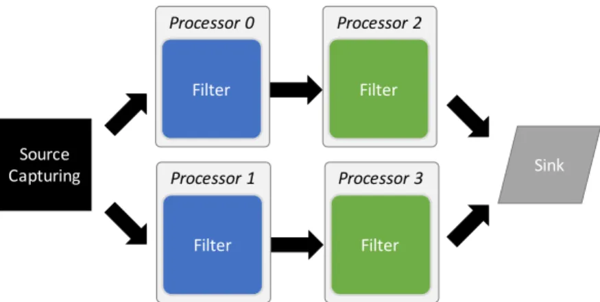
Due to increased computational demands, modern real-time systems now execute on multiprocessor platforms. Parallel programming of these platforms is required if applications are to exploit the extra available performance. The stream processing programming model [84] that consists of a collection of modules that compute in parallel and communicate via channels. Modules can be eithersource capturing(that pass data from a source into the system),filters

(that perform atomic operations on the data) andsinks (that either consume the data or pass it out of the system). Figure 1.1 is a simple illustration of stream processing.

Stream processing enables users to facilitate the construction of concurrent programs to exploit the parallelism available on multiprocessor architectures.

(22)

Processor 2 Processor 0

Filter Filter

Sink Source

Capturing Processor 1 Processor 3

Filter Filter

Figure 1.1: A stream processing example

Nowadays, stream processing has been widely adopted in different applica-tion domains, such as multimedia systems, signal processing systems, reactive systems, and Big Data systems [4, 5, 37, 44, 56, 64, 84, 87].

In addition to these stream processing frameworks, many programming languages also provide support for programming stream processing applica-tions. StreamIt [24] focused on developing a new language that was specifically designed for processing data streams on platforms ranging from embedded sys-tems to large scale and high performance syssys-tems. In addition, the most recent version of Java (Java 8) has introduced Streams and lambda expressions to support the stream processing paradigm, with functional-style code.

1.1

Motivation

Stream processing is suitable for several time-critical domains, such as real-time signal processing [62]. For example, an unmanned aerial vehicle (UAV) uses radar to identify potential obstacles and chose an avoidance path [77]. The continuous radar signals are processed by a on-board multiprocessor computer, and the processing is associated with real-time constraints to avoid potential hazards to the safety of individuals and communities. However, most stream processing architectures are not targeted towards real-time systems.

Often, many stream processing frameworks provide real-time performance by using high performance computation platforms, therefore increasing the speed of the stream processing so that the overall time which is required to handle the requests is reduced. Unfortunately, real-time guarantees are unlikely to be provided for every request using this approach even though

(23)

significant power and computation resources are employed. The reason is that these stream processing architectures pin their hopes on being sufficiently fast [85], rather than targeting towards real-time systems, to deliver “real-time” performance which is actually an illusion of real-time.

1.1.1 Real-time Stream Processing

Real-time stream processing systems are stream processing systems that have time constraints associated with the processing of data as it flows through the system from its source to its sink.

Typically, stream processing either divides incoming data into partitions and fully processes each partition before the next one arrives [22] (for example, object tracking, or radar beamforming), or directly operates on each incoming data items (for example, wheel speed sensor signals in a car’s ABS system). In the most general case, stream processing components may share the same computing platform, and interact with, other real-time components some of which might have hard real-time requirements.

In general, the data sources of stream processing systems can be classified into two types [71]: batched and live streaming.

• A batched data source is where the data is already present in memory, and its content and size will not change during processing.

• A live streaming data source represents data that arrives dynamically, its content and size will change with time.

The thesis intends to create an architecture using real-time principles, and implement a framework with real-time technologies, so that real-time guaran-tees can be provided to the stream processing.

1.1.2 Motivating Case Study

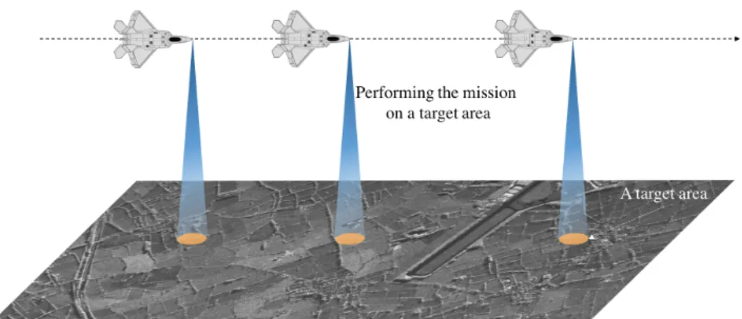
Consider an aircraft equipped with a spotlight synthetic aperture radar (SAR), and has a mission to generate images of a series of target areas using SAR, whilst its defence systems aim to guarantee its safety during the flight, as shown in Figure 1.2. According to the mission requirement, there is a real-time deadline for the imagery generation of each target area once the aircraft flies over it. At the same time, all the hard real-time tasks in the defence system must still meet their deadlines. All these tasks are executed by a multiprocessor mission control computer.

(24)

Figure 1.2: The mission of the generating images of target areas using SAR.

This is a scenario of the real-time stream processing, which inputs from a live streaming data source. However, it is difficult to employ existing stream processing techniques to generate images for each target area within the dead-line, whilst guaranteeing that all the hard real-time tasks in the defence sys-tem can still meet their deadlines. The reason is that these stream processing techniques are designed for time-sharing systems and so do not provide pre-dictability of execution. For example, there is no interface to configure the deadline for a job. More reasons are discussed in Chapter 2.

This case study will be addressed using our proposed real-time stream pro-cessing architecture in Section 5.6, along with its configuration. The derived response-time analysis guarantees that the time requirements of the mission are met.

1.2

Thesis Aims

The overall objective of the thesis is to develop a real-time stream process-ing architecture, and a prototype implementation, along with correspondprocess-ing schedulability analysis techniques. The challenges and contributions of the thesis are described in this section.

1.2.1 Challenges in Real-Time Embedded Stream Processing

Handling stream processing in a system that also host many hard real-time activities to meet the given time constraints, whilst the hard real-time com-ponents remain schedulable is challenging. The reasons include:

(25)

• Typically, the stream processing paradigm uses multiple processors in the system, and its input data source can be either static, i.e., a batched data sources or data which arrives dynamically, i.e., a live streaming data source.

– When processing a batched data source, how should the real-time stream processing of a batched data source be modelled into a real-time activity, so that the real-real-time characteristics, such as its dead-line, can be captured, and multiple processors can be utilised?

– For a live streaming data source, as each data item arrives dynam-ically, typically there is a deadline for completing each individual data item’s processing. Therefore, how to create a parallel real-time model to queue (if necessary) and process these data items within a stream processing paradigm also needs to be addressed.

• Stream processing is often computationally intensive, it can be either hard real-time or soft real-time. For the later case, it might be difficult to predict the volume and the cost of processing the data. If the stream processing activity is executed at a very high priority, it is likely to meet its deadline, but it may also cause hard real-time tasks in the same system to miss their deadlines. If the stream processing activity is assigned with a too low priority, such as the background priority, it may miss its target deadline because of suffering interference from higher priority hard real-time activities during its execution.

Therefore, how to execute a stream processing activity so that its dead-line can be met, whilst the hard real-time tasks remain schedulable raises another challenge.

• Another requirement for real-time stream processing is to derive appro-priate schedulability analysis. A real-time activity is schedulable if its response time is less or equals to its deadline. The response time is the time interval from when the input arrives to when the output is gener-ated in a system. Once the stream processing activity is executed by multiple processors, the worst-case response time of the stream process-ing is required to be calculated in order to test its schedulability.

(26)

– For a batched data source, the worst-case response time of the real-time activity which processes the whole batched data is required to be analysed.

– For a live streaming data source, as each data item is associated with a deadline, typically called latency, which represents the time from when the data arrived in the system to when the data pro-cessing has finished. Therefore, for every data item, the worst-case queueing time and response time of its processing is required to be analysed.

1.3

Thesis Hypothesis

This thesis addresses the hypothesis that:

Programming languages or existing frameworks’ support for stream processing is insufficient for addressing real-time require-ments. However, a generic architecture of a real-time stream pro-cessing infrastructure can be created to support predictable and analysable processing of both batched and live streaming data sources, and can be used in high-integrity real-time embedded sys-tems. Moreover, the architecture can be implemented as a frame-work using Java, with the Java Fork/Join frameframe-work and the Real-Time Specification for Java.

1.4

Success Criteria and Contributions

To assist with evaluating the work created as part of this thesis, the following success criteria were developed:

SC1 The definition of a generic architecture of a real-time stream processing infrastructure, which supports both batched data and live streaming data sources processing with real-time constraints, and is programming language independent.

SC2 A process for engineering time systems that have both hard real-time and hard or soft stream processing components, which focuses on how this architecture is to be mapped to the physical platform and how

(27)

the stream processing activity for both batched data and live streaming data sources is configured.

SC3 Response time analysis to determine the schedulability of stream pro-cessing for a batched data source, and latency for a live streaming data source.

SC4 A framework for integrating real-time stream processing activities with hard real-time components, and its implementation using the Real-Time Specification for Java (RTSJ).

SC5 An evaluation that demonstrates that the proposed model is as effective as a more typical real-time systems model that does not use the stream processing paradigm.

In addition to the above success criteria, a number of additional contribu-tions were also made during the development of this work. These were:

• The first use of execution-time servers for performing stream processing in the context of hard real-time control system.

• An algorithm for selecting the number of servers and their parameters, which maximises the processor time that can be allocated to real-time stream processing within the deadline, yet guarantees the deadlines of the hard real-time components.

• A bound task is free of ‘double-hit’ (see Section 5.1.1) introduced by higher priority deferrable servers, therefore maximising the capacity that can be reclaimed by deferrable servers. This observation has been proved, and is a supplement to the original RTA (as described in Section 5.1).

• A comparison of the relative efficiency of the Java and StreamIt stream processing models.

• An evaluation of the suitability of the Java stream processing framework for use within a real-time environment.

1.5

Structure of the Thesis

(28)

• Chapter 2provides some necessary background material before review-ing stream processreview-ing frameworks, and programmreview-ing languages.

• Chapter 3 described the architecture of a proposed real-time stream processing infrastructure, which enables processing both batched and live streaming data sources in real-time. This architecture is assumed by the proposed approach in Section 4, and analysis in Chapter 5. This chapter provides the material needed to meet SC1.

• Chapter 4presents the overall approach to configure and schedule real-time stream processing tasks for both batched and live streaming data sources to meet the real-time constraints. In addition, the assumptions we make on the underlying real-time platform are also described in this chapter. This chapter provides the material needed to meetSC2.

• Chapter 5 draw upon the research in schedulability analysis for the proposed real-time stream processing task model for both batched and live streaming data sources. An example of the scheduling, configuring and schedulability analysis for a real-time batched data processing task, and a case study of a real-time live streaming data processing application are also given in this chapter. This chapter provides the material needed to meetSC3.

• Chapter 6 investigates two different stream processing models, and describes the implementation (SPRY) of the architecture of the proposed real-time stream processing infrastructure using RTSJ, along with the implementation of the case study using SPRY. This chapter provides the material needed to meetSC4.

• Chapter 7 evaluates the presented real-time stream processing ap-proach to the traditional embedded apap-proach, when processing batched data and live streaming data sources. This chapter provides the material needed to meet SC5.

(29)

Chapter 2

Literature Review

This chapter first introduces some necessary background material on computer architectures and real-time in order to set the landscape within which this research has been conducted. A brief history of stream processing is then pre-sented. Several typical stream processing techniques, including frameworks, programming languages, are then reviewed in detail.

2.1

Parallel Computer Architectures

In recent years, processor manufacturers have turned to parallelism to speed up computation, rather than increasing the clock speed [54], and thus com-puters have evolved towards multiprocessor architectures. According to their memory access model, parallel computers can be classified into three typical architectures:

• Uniform Memory Access (UMA)

All the processors use the same memory, and they have equal access and access times to memory.

• Non-Uniform Memory Access (NUMA)

Processors are divided into groups, processors in each group access mem-ory using UMA. Not all processors have equal access time to all memo-ries. Cache Coherent NUMA (CCNUMA) is one type of NUMA archi-tecture that provides cache coherency. Most modern processors running on servers use this architecture.

• Distributed Memory

(30)

processors can not access data in other processor’s local memory. Pro-cessors communicate over networks.

This thesis is concerned primarily with UMA architectures. However, our underlying approach is also appropriate for NUMA architectures.

2.2

Real-Time Systems Model

The literature in real-time systems is broad. Here we present a top level view in order to place our work in context. More details will be given on particular techniques when they are used later in the thesis.

We introduce: the scheduling approaches used in the real-time literature, the problem of task allocation in a multiprocessor systems, and the role of execution-time servers.

2.2.1 Scheduling

The thesis focusses on the task-based scheduling of real-time systems, which have been summarised by Burns and Wellings [38]:

• Fixed-Priority Scheduling (FPS)

In a fixed priority scheduled system, each task has a fixed priority, which does not change with time. The tasks’ running order is determined by their priorities.

• Earliest Deadline First (EDF)

The running order of the runnable tasks is determined according to their absolute deadline, the task that has the nearest deadline executes prior to the rest of the tasks.

• Least Laxity (LL)

The runnable tasks are executed according to their slack, which is the deadline minus the required computation time. The next task to execute is the task with the shortest slack.

• Value-Based Scheduling (VBS)

This algorithm considers system where overloaded are possible. In this type of systems, each task is allocated with a value, and an online value-based scheduling approach is employed to determine which one is the next task to run. The one with the highest value is the one chosen.

(31)

In this thesis, we are concerned with priority-based scheduling as this is the most widely used approach [39] and the one supported by all real-time operating systems [38].

2.2.1.1 Preemption

In a preemptive system, when a higher priority task is released and a lower priority task is executing, the execution is immediately switched to the higher priority task. In contrast, in anon-preemptivesystem, the higher priority task has to wait for the lower priority task until it finishes its execution.

The preemptive scheme is adopted in this thesis as it makes higher priority tasks more responsive.

2.2.2 Task Allocation

Given a set of application tasks, a multiprocessor execution platform and preemptive priority-based scheduling, there are essentially three approaches to scheduling the tasks on the platform [38].

• Global Scheduling

A globally scheduled system is a system where all the tasks can execute on any available processor. A task that is executing on one processor can switch to another processor, i.e., a task can start its execution on one processor and then migrate to another process to continue/finish its execution.

• Fully-Partitioned Scheduling

A task in a fully partitioned system is not allowed to migrate to another processor once it has been allocated to one processor.

• Semi-Partitioned Scheduling

Semi-partitioned scheduling is between global scheduling and fully par-titioned scheduling. In a semi-parpar-titioned system, it limits which tasks may migrate, and where they may migrate to.

Normally, a single processor only resides in a single partition. This thesis addresses only Fully-Partitioned Systems as the schedulability analysis for such systems is a major domain in the real-time literature [38]. For example, in Chapter 5, we build our analysis on [47], which is based on fully-partitioned systems rather than globally scheduled systems.

(32)

2.2.3 Execution-Time Servers

In the real-time community, execution-time (or aperiodic) servers [38] are used to give tasks that might demand unbounded CPU time a good response time, while limiting their impact on other tasks so that, e.g., a hard real-time task will not miss its deadline. An execution-time server has a capacity, and a re-plenishment policy. When a client task execute under a execution-time server, it consumes the capacity. When the capacity is empty, the client task is not allowed to run and has to wait for the next replenishment.

For a periodic server [38], it has a capacity, which is periodically replen-ished. The capacity is consumed even if there is no client task. For example, a periodic server has a period of 10, capacity of 5, released at time 0. It has only 3 time units capacity left at time 12, because 2 time units capacity has idled away.

The POSIX standard supports Sporadic Servers [65,83]. A sporadic server has a replenishment period, a budget (or capacity), and two priorities: high priority and low priority. When handling aperiodic events, the server executes at the high priority when it has budget, otherwise runs at the low priority. When the server runs at the high priority, the amount of execution time that has been consumed is subtracted from its budget. The budget remains in-definitely if not consumed. If consumed, e.g., at time t, the budget will be replenished at t+ its replenishment period.

A Deferrable Server [65, 83] allows a new logical thread to be introduced at a particular priority level. This thread, the server, has a period and a ca-pacity. These values can be chosen so that all the periodic schedulable objects in the system remain schedulable even if the server executes periodically and consumes its capacity. When registered with a deferrable server, an aperiodic thread executes at the server’s priority level until either the capacity is ex-hausted or it finishes its execution. In the former case, the aperiodic thread is suspended or transferred to a background priority. The capacity of a de-ferrable server is replenished every period. Different from the periodic server, the capacity of a deferrable server is retained as long as possible, rather than idled away.

The response time of a task executing under an execution-time server can be analysed using the techniques provided by Davis and Burns [47]. The impact from a higher priority deferrable server to a lower priority task can be analysed by [34].

(33)

Processor 2 Processor 0

Filter Filter

Sink Source

Capturing Processor 1 Processor 3

Filter Filter

Figure 2.1: A stream processing example

In this thesis, we will use Deferrable Servers as they have superior schedu-lability compared to Periodic Servers. Furthermore, they are easier to imple-ment than sporadic servers. However, our framework is independent of the server technology used.

2.3

Stream Processing and Related Techniques

Stream processing has been around for decades, and is widely used in data flow systems, signal processing systems, reactive systems, etc. [1, 4, 12, 84, 87].

2.3.1 Stream Processing

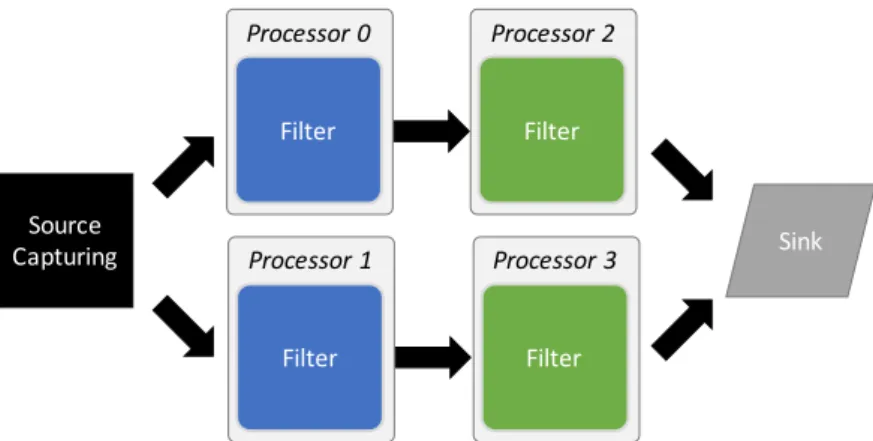
A stream processing system uses a collection of modules to compute the input in parallel, and communicates via channels [84]. Modules can be eithersource capturing (that pass data from a source into the system),filters (that perform atomic operations on the data) and sinks (that either consume the data or pass it out of the system). For example, a stream processing system that has 4 filters computing in parallel can be illustrated in Figure 2.1 (a replication of Figure 1.1 for convenience of presentation). The filters in processor 0 and 1 have the same functionality, and their outputs flow into filters in processor 2 and 3 separately.

2.3.2 Stream Processing Data Source Classification

As has been introduced in Section 1.1.1 the data sources of stream process-ing systems can be classified into two types [71]: batched and live streaming.

(34)

Note however, the live streaming data may has other names, for example, in Big Data community, the live streaming data is also called real-time data. However, the real-time in this thesis represents “any information processing activity or system which has to respond to externally generated input stimuli within a finite and specified period” [38]. For the clarification, the term live streaming used to to represent this type of data sources.

2.3.3 A Brief History of Stream Processing Techniques

The earliest recorded work of stream processing is data flow programming in 1960s [84], even though it was not termed as data flow at that time. Then, several research projects targeting stream processing were performed. For ex-ample, in 1970s, Kahn Process Networks were proposed as an asynchronous programming model for data flow, i.e., filter processing without synchronisa-tion with respect to other filters. Synchronous data flow [64] was proposed in 1980s for stream processing, where synchronisation was supported when col-laboration between filters is required. In 1990s, LUSTRE [57] was proposed as a programming language to support synchronous data flow. More related stream processing work in the past decades is reviewed in [84].

In 2002, StreamIt [87] was created as a new language for stream processing on platforms ranging from embedded systems to large scale and high perfor-mance system. In 2003, Brook [36] was proposed as a stream processing spec-ification, and its main follow-up work is Brook for GPUs [37], which was de-veloped for the stream processing on GPUs. In the same year, STREAM [28], Aurora [26], and Medusa [43] were created to support stream processing mainly in data management systems.

In order to address the requirement of large data sets processing in a distributed computer cluster, MapReduce [50] was announced by Google in 2004. MapReduce partitions the input, distributes the partitions over the computer clusters, performs operations, and fold the results. In addition, Borealis [5] integrated Aurora [26] and Medusa [43] to provide a distributed stream processing system for data management.

In 2007, Microsoft announced Dryad [60], which supports distributed large data sets processing with directed acyclic graphs (DAG) so that more com-plicated processing logic can be represented. Inspired by StreamIt, Stream-Flex [82] was also proposed in 2007, which intends to deliver low-latency stream processing. StreamFlex uses abstractions supported by the Real-Time

(35)

Specification for Java (RTSJ) [91], e.g., a memory area that avoids any inter-ference from garbage collectors, to minimise latency.

In 2008, DryadLINQ [93] was proposed to provide a high level language abstraction, which enables the succinct description of a distributed stream pro-cessing job. In 2010, FlumeJava [41] was created to provide an easy, efficient data parallel pipeline, which was used by Google internally.

In 2010, S4 [76], and Storm [4] were proposed for distributed live stream-ing data processstream-ing. Spark [1] was created to support in-memory stream pro-cessing of large data sets. In addition, MapReduce online [45], Twister [52], HaLoop [35] also tried to refine MapReduce so that it can be used iteratively, in order to provide interactive data processing. In addition, considering the requirement of large-scale graph processing, such as, social networks that has billions of vertices, trillions of edges, Pregel [69] was proposed by Google.

Spark Streaming [19] was developed as a library on Spark in 2013, in order to support live streaming data sources. In the same year, MillWheel [27] was also created at Google, to support live streaming data processing as MapRe-duce is not fit for live streaming data. Additionally, Flink [40], Heron [61], and Samza [2] were developed in 2014 to 2015 as distributed stream process-ing frameworks, in order to deliver more scalability and efficiency compared to Storm. In addition, inspired by FlumeJava [41] and PLINQ [15] that provides a parallel implementation of data set operations, Java SE 8 [12] was released in 2014, with Java 8 Streams and lambda expressions, which enables efficient parallel stream processing with functional-style code.

These stream processing techniques introduced above are designed for best effort, time-sharing systems. For time systems, some distributed real-time frameworks have emerged in recent years, for example, [33] is a real-real-time version of Storm [4], and the JUNIPER [31] project. These frameworks provide supports to process large data sets in a distributed computer cluster, with a predictable processing time. However, it is difficult to implement a hard real-time system in a distributed system, because of the unpredictability of the network, they are targeted soft real-time.

2.3.4 Stream Processing Classification

In the most recent stream processing frameworks [1,4,12], stream processing is typically represented by a pipeline with zero or more synchronous stages. Each stage contains one or more filters, which are allocated to different processors

(36)

Filter 1 Filter 2 Filter 3 Filter 4 Sink Source

Figure 2.2: A pipeline that has 4 filters

X->X+1 X->X*2 X->X-1 X->X2 _Sink

1 2 4 3 9

(a) Eager evaluation of a pipeline.

X->X+1 X->X*2 X->X-1 X->X2 _Sink

Source

1 9

(b) A pipeline that is lazily evaluated.

Figure 2.3: The evaluation of a pipeline.

or computer nodes to execute, in order to exploit the possible parallelism. The whole processing procedure forms a DAG.

According to the executing behaviour and allocation of the filters, stream processing can be classified into different types. Considering a typical pipeline, which contains 4 filters can be illustrated by Figure 2.2, the stream processing can be classified as:

• Lazy or Eager

According to the behaviours of the pipeline’s executing, their evaluation can be classified as eagerly, and lazily.

– Eager Evaluation

The input is processed eagerly in this model, i.e., any filter in this model triggers the processing immediately. When an input arrives at a pipeline that is eagerly evaluated, the input is immediately processed by the first filter, and generates an intermediate result, which will be an input of the down stream (or next stage) filter. The intermediate results are typically transferred via channels, shared memory buffers, or networks in a distributed computer cluster. This model can be illustrated by Figure 2.3a, where a pipeline that contains four filters is used to process numbers. For example, when the number1enters the eager evaluated pipeline, it is immediately processed by the filter that increases the input by 1, and generates

(37)

2 as the intermediate result. The intermediate result2 is then be sent to the next filter that multiplies the input by 2, and we get the number4. So on and so forth. In this example, three intermediate results are generated, stored and transferred by channels.

– Lazy Evaluation

In a lazily evaluated model, the processing or the input is delayed as long as possible, and only processed when necessary, such as, when the final results are requested or the intermediate results are required to be transferred to another machine in a distributed en-vironment.

Considering the same pipeline again, Figure 2.3b illustrates how it is lazily evaluated. When the input 1 arrives, it is not processed until the sink requests the final result. The filters are combined together to be a super filter, so that the input is processed by this super filter, and no intermediate result is generated or transfered. Lazy operations not only can avoid unnecessary evaluation, but also can provide potential optimisation opportunities. For example, the following Java 8 pseudo code gives the MD5 hash code of the first number in a given array. Lazy operations enables a return generated upon the first input, instead of calculating all numbers’ hash code then finding the first one.

Arrays.stream(new int[] { 1, 2, 3,..., 1000000 }) .map(n -> MD5(n))

.findFirst()

.ifPresent(System.out::println);

However, a lazy pipeline is identical to a eager pipeline when the intermediate results of each filter are required to be transferred to another machine. Typically, when evaluating a lazy pipeline, the application travels through the pipeline until a filter that triggers the processing is met. Then the application travels back to the first filter and perform operations in down-stream filters one by one. Compared to a eager pipeline, this introduces overheads when there is no optimisation opportunities.

• Control Parallel or Data Parallel

(38)

Fig-Waiting Queue i i i i 4 3 1 2 1 1 1 1 2 2 2 2 4 2 3 3 4 4 3 3 3 3 4 4 4 4 0 1 2 3 4 5 6 7 8 9 Processor 0 Processor 1 Processor 2 Processor 3 Time

Filter 1 processing data i Filter 2 processing data i Filter 3 processing data i Filter 4 processing data i

Figure 2.4: A control-parallel pipeline.

ure 2.2 again, and a 4 processors SMP CPU. The inputs are 4 data items, which arrive at time 0, and are stored in a waiting queue.

According to the processor allocation, a pipeline can be either mapped across different processors, i.e., control parallel, or duplicated on each processor, i.e., data parallel.

– The Control-Parallel Pipeline

The control-parallel pipeline behaves similar to an instruction pipe-line within a modern CPU. In this scheme, one or more filters are mapped to a processor, but a same filter does not reside on more than one processor. In this example, each filter is mapped to dif-ferent processors as shown in Figure 2.4. The processor 0 takes an input from the waiting queue, processes it, passes the intermediate result to the down-stream filter that is running on processor 1, then takes another input from the waiting queue. Note that, the result merging is not shown.

Multiple processors can be utilised to exploit the parallelism, how-ever, the control-parallel pipeline has the following disadvantages:

∗ When the pipeline contains too few stages compared to the number of available processors, some of the processors cannot

(39)

Waiting Queue 4 3 1 2 1 1 1 1 2 2 2 2 3 3 3 3 4 4 4 4 Processor 0 Processor 1 Processor 2 Processor 3 i i i i 0 1 2 3 4 5 6 7 8 9 Time

Figure 2.5: A data-parallel pipeline.

be utilised, therefore, making the system inefficient.

∗ If the pipeline is unbalanced (i.e., computation time, of each fil-ter is not identical), or up-stream filfil-ters’ processing is delayed, for example, due to receiving interference from other activities, the system efficiency is reduced. The reason is that, when any up-stream filter requires more time to finishes its processing, the down-stream filter has to wait for it idly.

∗ Moreover, inter-processor communication introduces extra over-heads.

– The Data-Parallel Pipeline

The data-parallel pipeline duplicates the entire pipeline to different processors, as shown in Figure 2.5. The data is allocated to different processors. In this example, each processor works independently, and there is no waiting gap. The data-parallel pipeline is suitable for lazy evaluation, as all the filters are allocated into the same processor. Again, the result merging is not shown in the figure. However, the drawback of a data-parallel pipeline is making the the pipeline span different computation resources impossible. For example, one of the filter within the pipeline requires to access a GPU or FPGA.

(40)

Filter 1 Filter 2 Filter 3 Filter 4 Sink

Source Filter 5 Filter 6

(a) The pipeline used in the hybrid pipeline example.

Stage 1 5 5 5 5 6 6 6 6 7 7 7 7 8 8 8 8 Processor 4 Processor 5 Processor 6 Processor 7 Waiting Queue 4 3 1 2 1 1 1 1 2 2 2 2 3 3 3 3 4 4 4 4 0 1 2 3 4 5 6 7 8 9 Processor 0 Processor 1 Processor 2 Processor 3 Time i i i i

i Filter 5 processing a data collection

i Filter 6 processing a data collection

8 7 5 6

Stage 2 2 _{Waiting Queue} 3 1 4 Processor 8 1, 2, 3, 4 Processor 9 8 7 5 6 5, 6, 7, 8 1, 2, 3, 4 5, 6, 7, 8 4 5 6 7 8 9 10 11 12 Time 13 14

(b) The processing of the example hybrid pipeline.

Figure 2.6: The hybrid pipeline.

– The Hybrid Pipeline

With a hybrid pipeline, the pipeline can span different nodes in a distributed system, while within each node, the pipeline is dupli-cated according to its data source partitions.

For example, a hybrid pipeline can be illustrated by Figure 2.6. Where the logic of the pipeline is shown in Figure 2.6a, the pro-cessing of this pipeline is illustrated by Figure 2.6b. This example inputs data collections, which are firstly processed by the first 4 filters using a data-parallel model. For example, the first input col-lection 1,2,3,4 are partitioned, and processed by processor 0, 1, 2, and 3. This can be illustrated as stage 1 in Figure 2.6b. The in-termediate results are merged, and sent to down-stream filters. For example, the merged intermediate results are then processed by fil-ter 5 and 6 using a data-parallel model, with processor 8 and 9. This can be illustrated as stage 2 in Figure 2.6b. The sub-pipelines in Stage 1 and 2 are evaluated using a control-parallel model.

(41)

processing techniques that were discussed previously. A summary of those techniques and their characteristics is given in Table 2.1. The remainder of this subsection justifies our choice of the set of representative techniques to consider.

Table 2.1: Stream Processing Techniques Classification

Technique Type Behaviour Pipeline Type RT StreamIt Language Eager Control parallel No

Spark Framework Lazy Hybrid No

Java 8 Streams Framework Lazy Data parallel No

Storm Framework Eager Hybrid No

JUNIPER Infrastructure Hybrid Hybrid Soft RT-Storm Framework Eager Hybrid Soft

StreamIt is chosen as it targets embedded systems and provides flexible support for the development of stream processing applications [87]. It uses an eager pipeline as any filter triggers the processing, and a control-parallel model. It is also a widely referenced stream processing language.

In order to address the requirement of large data sets processing chal-lenges introduced by the rapid growth in data production, MapReduce [50], Hadoop [3], and Dryad [60] were created. Recently, Spark [1] has success-fully succeeded these frameworks. Spark uses lazy evaluations (as only certain types of filters trigger the processing), and a hybrid pipeline. We, therefore, review Spark as an example of a batched stream framework for large scale data processing applications.

Java is a popular programming languages, and used widely in modern stream processing domain, for example, Hadoop, Spark, Flink [40], Storm, etc., are based on Java platforms. In the most recent version (Java 8) a stream processing library has been included to support efficient batched data stream processing in parallel. Java 8 Streams are lazily evaluated, with a data-parallel pipeline. Java is reviewed as it is used in this thesis to implement our proposed real-time stream processing architecture. It is also an example of a framework that supports batched stream processing.

Storm [4] was created to target live streaming data processing, and has been widely adopted in commercial areas [90]. Storm is considered because the hybrid pipeline model, and uses the eager evaluation model (because any filters

(42)

in Storm triggers data processing). Storm is, therefore, reviewed as an example of a commercially successful live streaming data processing framework.

In order to address the real-time requirement of stream processing, JU-NIPER [31] and a real-time version of Storm [33] were created. JUJU-NIPER mainly targets batched data processing in real-time, while real-time Storm focuses predictable live streaming data processing. We consider these two as they are two state-of-the-art frameworks that focus on real-time streaming issues (albeit in a distributed environment).

2.3.5 StreamIt

StreamIt [87] is mainly based on Java, but provides its own compiler (it com-piles StreamIt source code to Java code, then translates the Java code to C++ code using a third party library, and finally generates a binary executable file using G++) and tool set. StreamIt defines several concepts. The basic con-cept is the filter, which is a computation unit of StreamIt, and contains user defined data processing code. StreamIt also defines global variables, that can be accessed by any of the filters.

A simple stream processing program can be defined using the following StreamIt code:

void->void pipeline Example() { add IntegerSource();

add IntegerPrinter(); }

void->int filter IntegerSource { int i;

init { i = 0; }

work push 1 { push(i++); } }

int->void filter IntegerPrinter { work pop 1 { print(pop()+" "); } }

This program defines a pipeline, which contains two filters:

- the IntegerSource filter, which takes nothing as the input, and gener-ates an incremental integer each time (via the “push” statement). The push statement writes the results into the communication channel.

(43)

“pop” statement), and prints it out. The pop statement reads numbers of intemediate results from the communication channel.

The program is controlled by a loop, with a user configured total iteration times. Within each iteration, an input is read into the system, and then sent to the down-stream filters for processing. For example, after compilation, the user can run this program with the following command:

./Example -i 5

The program iterates 5 times, and generates the output: 0 1 2 3 4.

2.3.5.1 Connecting the Filters

The notion of stream in StreamIt is defined as a component, which has one or more connected filters and with data flows into and out. Three structures of stream processing logic are defined by StreamIt, by connecting filter in different ways: the Pipeline, theSplitJoin, and theFeedbackLoop.

Pipeline

The Pipeline is used to construct a sequential stream, which has a series of filters connected linearly using the add command (see line 2, and 3 in the above code). An example of the pipeline has been introduced above.

SplitJoin

The SplitJoin splits the input data stream to different branches, which can process data items in parallel, and merge the intermediate results into a com-mon joiner. For example, the following code distributes the input to two filters in a round-robin fashion.

void->void pipeline SJExample() { add IntegerSource();

add SJ(); add Printer(); }

void->int filter IntegerSource { int i; init { i = 0; }

work push 1 { push(i++); } }

int->int splitjoin SJ () { split roundrobin;

(44)

X->X+1 X->X+2 X->print(x) 0 Integer Source 1 1 3

Figure 2.7: StreamIt SplitJoin example, the cycle with numbers represent the input data or an intermediate result.

add Adder(1); add Adder(2); join roundrobin; }

int->int filter Adder(int increment) {

work pop 1 push 1 { push(pop()+increment); } }

int->void filter Printer {

work pop 1 { print(pop()+" "); } }

The program can be illustrated by Figure 2.7. Run the program with 2 iterations, the source generates the input (i.e.,0), and the second input (i.e.,

1). The first input is sent to the filter: x−> x+ 1, while the second input is sent to the filter: x−> x+ 2. Finally,1 3is printed.

StreamIt supports three types of SplitJoin:

1. Duplicate

Each input is duplicated, and sent to every added filter.

2. RoundRobin

The inputs are distributed to added filters in a round-robin fashion. The first data is sent to the firstly added filter, the next data is sent to the secondly added filter, and so on.

3. Null

It considers the parallel paradigm where there is no input is required by the added filters.

(45)

FeedbackLoop

The FeedbackLoop is used to create cycles in the stream processing graph. For example, a stream that calculates the Fibonacci numbers can be described by the following example, which is taken from StreamIt benchmarks [23]. The feedbackloop takes two numbers each turn, generates the output by adding them together. The output of the feedbackloop is copied to 2 pieces: one goes to the printer, one is go back to the feedbackloop as an input in the next iteration.

void->void pipeline Fib { add feedbackloop { join roundrobin(0, 1); body PeekAdd(); split duplicate; enqueue 0; enqueue 1; }; add IntPrinter(); }

int->int filter PeekAdd { work push 1 pop 1 peek 2 { push(peek(0) + peek(1)); pop(); }

}

int->void filter IntPrinter { work pop 1 {

println(pop()); }

}

2.3.5.2 Parallel/Distributed Execution

StreamIt is supported on Linux. The StreamIt compiler compiles the code into Java source code, and then generates C code. Finally, the C code is compiled into binaries using GNU G++.

(46)

Processor Allocation

When compiling a StreamIt program, the number of processors that are allo-cated to the program is required to be given, otherwise, by default, the code is compiled to be a sequential program. In addition, there is also a configuration file, which specifies the host, i.e., which node in a computer cluster, where each processor is located in.

Each filter in the code is compiled to be a C function, and the data flow between two filters is implemented using shared memory buffers in a multi-processor CPU, or TCP/IP sockets in a distributed system.

When there are more filters than processors, the StreamIt compiler com-bines several filters to be a super filter. The compiler generates several super filters as many as the available processors. These super filters are allocated to POSIX threads for execution.

However, when there are more processors than filters, some of the unallo-cated processors are idle as StreamIt does not duplicates filters.

Performance Optimisation

The StreamIt compiler estimates the computation load of each filter using simulation, then allocates different numbers of filters into different super filters so that the super filters have an identical amount of computation load.

In addition, StreamIt also employs function inlining, array scalarization, and loop unrolling to optimise the performance [55].

2.3.5.3 Discussion

StreamIt is a stream processing programming language, which enables data flow processing program can be written using concise code.

However, the main drawback of StreamIt is that it is a special purpose language, so that it is hard to integrate with general purpose languages.

In addition, the pipeline in StreamIt is not replicated by default. There-fore, when there are more processors, it relies on users to construct a parallel structure, which can utilise all the processors. For example, it assumes users will use the SplitJoin to duplicate the filters. Otherwise, some of the processors are idle.

As StreamIt is not designed for real-time systems, it is impossible to be directly integrated with real-time systems. This is because the threads may

(47)

demand unlimited CPU time, therefore causing the hard real-time tasks in the same system to miss their deadlines.

2.3.6 Spark

Spark [1] was created at UC-Berkeley and implemented in the Scala program-ming language, which runs on the JVM and targets batched data processing. Spark provides a functional programming interface, which enables program-ming with concise code. Spark Streaprogram-ming [19] is an extension of Spark, and allows the live streaming data to be processed using the existing Spark run-time.

The data structure used by Spark is the Resilient Distributed Dataset (RDD), which represents a read-only collection of data located in a set of machines. Data that is corresponding to the RDDs can be parallel processed by invoking multiple parallel operations, for example, map, reduce etc. An example is described by the following Scala code:

1val InputFilesRDD = spark.textFile("hdfs://...")

2val ResultRDD = InputFilesRDD.flatMap(line => line.split(" "))

3 .map(word => (word, 1))

4 .reduceByKey(_ + _)

5//save the result...

In this example, a RDD named InputFilesRDD is created from the text files that are stored in HDFS (see line 1). The InputFilesRDD references to all the texts in these text files. Spark splits each line into words using theflatMap operation (see line 2), and these words are represented by a new RDD. Each word in this new RDD is mapped into pairs(word,1) by invoking the map operation (see line 3), and the generated pairs are represented by another newly created RDD. Spark performs the reduceByKey operation on this RDD, and generates the final result.

The Spark application runs as a set of Java JVM processes on a cluster, with a master-slave architecture.

2.3.6.1 The Resilient Distributed Dataset (RDD)

An RDD is a read-only, distributed, partitioned collection of records, and it is the core concept of Spark [95]. An RDD is an object that references the data source, and provides several parallel operations for data processing. Zaharia

(48)

Figure 2.8: Spark Streaming Overview [20]

claims that RDDs are so general that RDDs can emulate any distributed system [94].

RDDs can be created by invoking deterministic operations on either data in stable storage or other RDDs. The RDDs are lazy evaluated, which means that the data is evaluated only whenaction operations(they are similar to terminal operations defined in Java 8) are invoked, rather than all of the operations in pipeline are performed on data immediately. In addition, programmers can call apersist method to indicate which RDDs are going to be reused in future. Spark also connects and performs multiple operations in a pipeline on RDDs to optimise the performance, in the same machine. For example, RDDs can be evaluated by applying amapfollowed by afilter operation on the same node. Thus, transferring the intermediate results among nodes is avoided.

2.3.6.2 Spark Streaming

Spark Streaming is an extension to Spark, which is designed for live streaming data processing. The core concept of Spark Streaming is Discretized Streams (D-Streams), which were created in order to enable the Spark to provide live streaming data items with an interactive response time. By using D-Streams, a DAG can be created to represent the processing logic.

The key idea of Spark Streaming is that D-Streams treats a live streaming computation as a series of deterministic batch computations on small time intervals [96]. For example, in order to process live streaming data, we can group data received every second into a batch, and processes each batch using Spark. This can be shown in Figure 2.8, Spark streaming groups live streaming data into batches periodically, and processed using the existing Spark runtime.

(49)

Figure 2.9: Structure of D-Streams [20]

Figure 2.10: Applying the flatMap operation on a D-Streams [20]

The D-Streams Computation Model

A D-Stream is a sequence of immutable, partitioned datasets (RDDs) that can be parallel processed by numbers of operations [94]. These operations can yield new D-Streams or generate outputs, and any operation that is applied on Stream will be translated to operations on the underlying RDDs. In a D-Stream, each RDD contains data from a certain interval. Figure 2.9 illustrates the structure of a D-Stream, in this example, the D-Stream consists of RDDs with the period of 1 second. For example, in the WordCount example, the first stage is converting a stream of lines to words. The lines D-Stream is transformed by a flatMap operation, as described by Figure 2.10. Each RDD in the lines D-Stream is evaluated by the flatMap operation, and the RDDs representing the words are generated. Finally, the newly generated RDDs form the words D-Stream. In this example, the Spark Streaming framework generates a batch processing task (i.e., underlying RDD transformations) every second, and these tasks will be processed by the Spark Engine.

(50)

2.3.6.3 Scheduling Spark Applications

By default, Spark schedules applications in FIFO order, each application are allocated with a fixed amount of resources (the number of processors and the size of memory). Dynamic resource allocation is introduced in Spark version 1.2. This approach allows an application to give resources back to the scheduler when it does not use them, and request resources again later when needed. For example, when some tasks within an application are waiting for I/O, the processors that are allocated to these tasks can be given back to the scheduler temporarily.

2.3.6.4 Scheduling Within The Spark Application

Spark hides the details of resource allocation for the pipeline, for example, how many workers are involved by each operation. Spark uses the following concepts and schemes to execute a pipeline in parallel, or in a distributed system.

A Spark application may generate several RDDs as the results. Addi-tionally, one or more operations in a pipeline and source RDDs are used to generate each target RDD.

In Spark, responding to a Spark action, e.g., generating a target RDD, is defined as a job. Each job will be compiled into multiple tasks. The task in Spark is executable code, typically part of the code within an operation, e.g., the processing logic in a map operation. The tasks are executed by the executors, which are JVM processes running the worker node. This section describes how a job is compiled to tasks, and how Spark executes these tasks. When an RDD is required to be generated, i.e., a job is generated, the scheduler examines all the operations and required input RDDs, then builds multiple stages to execute this job. Stages are generated using the following principles:

• Each stage should contain as many pipelined operations with narrow dependencies as possible. The narrow dependencies are the relationship in where multiple operations on a RDD can be composed together into a single operation. For example, in WordCount, there are two opera-tions: mapping lines to words, and mapping words to (word,1) pairs. These two operations can be put into a single operation, because the data/partitions is transformed in a one-to-one relation.

(51)

Figure 2.11: The stages in a job. Boxes with solid outlines are RDDs, Shaded rectangles are partitions, black rectangles means partitions are already in memory. [94]

• The boundaries of the stages are either the shuffle operations, or any already computed partitions, which determines that their parent RDD is not required to be computed.

Figure 2.11 illustrates an example of how Spark determine the stages of a job. In this example, in order to generate RDD G, Spark builds three stages according to the above principles:

1. Stage 1

The goal of it is to generate RDD B. Note that, in this example, the results have been generated.

2. Stage 2

The goal of this stage is to generate RDD F. The map and union op-erations in this stage represent a one-to-one relation, therefore, Spark merges them in the same stage for the optimisation.

3. Stage 3

In this stage, the join operation is required to be performed on RDDB

and RDDF, and then generate the finally required result, i.e., RDD G.

As the output RDD of stage 1 is already in memory, therefore Spark runs stage 2, then stage 3. Once the stages are determined, the scheduler generates tasks, which are to compute the missing partitions for each stage. Finally, the target RDD is computed.

(52)

The number of tasks spawned by each stage equals to the number of par-titions from the target RDD within this stage. In this example, 4 tasks are generated in stage 2, 3 tasks are generated in stage 3, and 1 shuffle task are created between stage 2 and 3.

The tasks will be executed by executors, which are JVM processes. The total number of number of executors, and processors that each executor can use is configured when the application is deployed.

Scheduling The Generated Jobs

The default scheduler is a FIFO scheduler. When scheduling jobs, the first arriving job has the highest p