Representations
Mateo Rojas-Carulla
Department of Engineering University of Cambridge
This dissertation is submitted for the degree of Doctor of Philosophy
I hereby declare that except where specific reference is made to the work of others, the contents of this dissertation are original and have not been submitted in whole or in part for consideration for any other degree or qualification in this, or any other university. This dissertation is my own work and contains nothing which is the outcome of work done in collaboration with others, except as specified in the text and Acknowledgements. This dissertation contains fewer than 65,000 words including appendices, bibliography, footnotes, tables and equations and has fewer than 150 figures.
Mateo Rojas-Carulla September 2018
The journey towards this thesis would not have been possible without the outstanding scientists and friends that I encountered along the way.
Bernhard Schölkopf provided me with encouragement through stressful periods, gave me constant support and freedom to pursue open research questions. Richard Turner taught me how to tackle a scientific question in a principled manner; his optimism and kindness are unmatched and always made things better. Jonas Peters was key in shaping my critical thinking and made a better scientist out of me, I am forever grateful.
Ilya Tolstikhin, a dear friend and mentor, helped make my stay at the Max Planck into some of the best years of my life. His desire to learn and improve, as well as his dedication to family and friends, make him a role model in science and in life.
I have been fortunate to be surrounded by amazing people who have contributed in ways which are hard to express. Niki Kilbertus and Giambattista Parascandolo taught me that science benefits from a great team and that fun and curiosity should drive research. Sebastian Gómez’s optimism and values were always an inspiration and provided much needed support.
I am thankful toDavid Lopez-Paz, from whom I learned scientific practices I now follow, and Marco Baroni, who was kind enough to provide his time and invaluable feedback.
Cambridge and the Max Planck are wonderful first and foremost because of their outstand-ing members, who have contributed to make me into a better person and a better scientist, includingDiego Agudelo, Carl-Johann Simon-Gabriel, Niklas Pfister, Paul Rubenstein, Stefan Bauer, Dieter Büchler, Okan Koc, Yassine Nemmour, Vinay Jayaram, Eduardo Pérez, the CamTue crowd, and many others.
Receiving my PhD would not have been possible without people who taught me the foundations and ignited my desire to learn and keep asking questions. I would particularly like to thank Stephan Céroi, who gave me a strong mathematical foundation in high school, Régine Astruc, a great teacher who supported me during the difficult yet exciting years of prépa, and Jean-Luc Vidal, who provided invaluable guidance.
I am forever grateful to Kata, who put up with me during the writing of this thesis and has brought so much wonder and joy into my life. Last but not least, I dedicate this thesis to my amazing family, to whom I owe everything I have achieved and who bring to life the meaning of unconditional love.
A first contribution of this thesis is to propose causality as a language for problems of distribution shift. First, we consider domain generalisation, where no data from the test distribution are observed during training. What assumptions can be made regarding the relation between train and test distributions for transfer to succeed? We argue that assuming the data in both tasks originate from the same causal graph leads to a natural solution: use only causal features for prediction, as the mechanism mapping causes to effects is invariant to shifts in the probability distributions induced by the causal structure. We provide optimality results when the test task is adversarial, and introduce a method for exploiting all remaining features when data from the test task are observed. We motivate that learning such invariant mechanisms mapping features to outputs leads to machine learning modules robust to transfer.
Second, we consider a classification problem where only few examples are available for each label. How should an initial large dataset be leveraged to improve performance in this task? We argue that such a dataset should be used to learn powerful features for batch classification using a neural network. We present a framework which transfers between classes by building a probabilistic model on the weights of the network. Our results suggest that practitioners should use the original dataset for building features whose power can be exploited during few-shot learning.
Finally, we extend causal discovery to solve problems such as distinguishing a painting from its counterfeit. Given two such static entities, a proxy random variable introduces the randomness necessary to construct two features of the static entities which preserve their causal footprint, measurable by a standard causal discovery procedure. Experiments on vision and language provide evidence that the causal relation between the static entities can often be identified.
List of figures xv
List of tables xvii
List of notations xix
1 Introduction 1
1.1 Outline and Contributions . . . 3
2 An Overview of Causal Inference 7 2.1 Fundamental Technical Notions . . . 8
2.1.1 From Statistical to Causal Dependence . . . 8
2.1.2 Directed Acyclic Graphs, Structural Equation Models . . . 9
2.2 Observational Causal Discovery . . . 11
2.2.1 Additive Noise Models . . . 12
2.2.2 Training Based Methods . . . 13
2.3 Causal Inference Using Invariant Predictions . . . 13
2.4 Causality in Machine Learning . . . 15
3 Invariant Causal Representations for Transfer Under Distribution Shift 17 3.1 An Overview of Distribution Shift . . . 18
3.1.1 From Standard Machine Learning to Distribution Shift . . . 18
3.1.2 Measuring Differences Between Distributions . . . 22
3.1.3 Assumption For Distribution Shift . . . 25
3.2 Invariant Models for Domain Generalisation . . . 29
3.2.1 Assumption for Domain Generalisation . . . 31
3.2.2 Proposed Estimator . . . 33
3.2.3 Optimality in an Adversarial Setting . . . 34
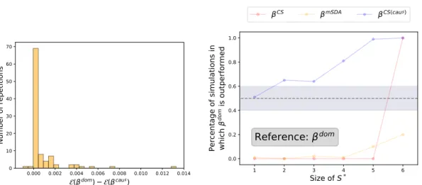
3.2.4 Comparison Against Pooling the Data . . . 36
3.2.5 Relation to Causality . . . 39
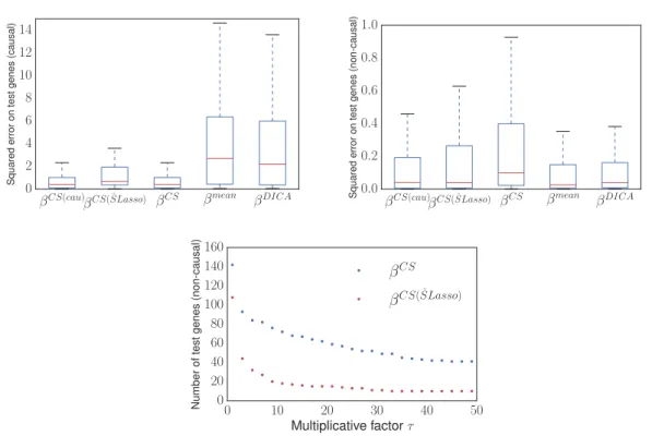
3.2.7 Synthetic Data Experiment . . . 44
3.2.8 Gene Perturbation Experiment . . . 49
3.3 Learning Representations for Multi-task Learning . . . 53
3.3.1 Learning Features Via a Missing Data Approach . . . 54
3.3.2 Synthetic Data Experiment . . . 59
3.4 Learning Independent Causal Mechanisms . . . 62
3.4.1 Learning Inverse Feature Mappings with Competition . . . 64
3.4.2 Experimental Results . . . 65
3.5 Conclusion . . . 70
4 Learning Representations for Few-shot Learning 73 4.1 Introduction . . . 73
4.1.1 Few-shot Learning Setting . . . 74
4.2 Methods for Few-shot Learning . . . 75
4.2.1 Meta-learning Methods . . . 75
4.2.2 Deep Probabilistic Methods . . . 78
4.3 Probabilistic Few-shot Learning . . . 79
4.3.1 A Framework for Probabilistic Few-shot Learning . . . 81
4.3.2 Choosing a Model for the Weights . . . 84
4.3.3 Relation to Logistic Regression . . . 87
4.3.4 Calibration of a Classifier . . . 88
4.4 Experiments on Image Classification Tasks . . . 89
4.4.1 Model Assessment on CIFAR-100 . . . 89
4.4.2 Experiments on miniImageNet . . . 93
4.5 Conclusion . . . 99
5 Learning Representations Preserving Causal Footprints 101 5.1 The Concepts: Static Entities, Proxy Variables and Proxy Projections . . . . 102
5.2 Causal Discovery Using Proxies in Images . . . 104
5.2.1 Analysis in a Special Case . . . 106
5.2.2 Numerical Experiments . . . 107
5.3 Causal Discovery Using Proxies in Language . . . 108
5.3.1 Causal Discovery in NLP . . . 109
5.3.2 Static Entities, Proxies, and Projections for NLP . . . 110
5.3.3 A Real-World Dataset of Cause-Effect Words . . . 112
5.3.4 Experiments . . . 112 5.4 Conclusion and Thoughts for Proxy Variables in Broader Machine Learning . 116
6 Discussion and Conclusion 119
6.1 Causality as a Language for Transfer . . . 119
6.2 Modularity of Causal Mechanisms and Assumptions . . . 121
6.3 For Few-shot Learning, Learn the Best Possible Features . . . 121
6.4 Empirically, Features Extracted from Static Entities Preserve the Causal Footprint . . . 122
References 125 Appendix A Architecture Details for the Competition of Experts 133 Appendix B Datasets and Architectures for Few-shot Learning 135 B.1 Dataset Details for CIFAR-100 . . . 135
B.2 Dataset Details for miniImageNet . . . 136
B.3 Network Architecture and Training: ResNet Inspired . . . 136
B.4 Network Architecture and Training: VGG Inspired . . . 136
Appendix C Instructions for Creating the Dataset of Word Pairs 141 C.1 Instructions for Word Pair Creators . . . 141
2.1 An Additive Noise Model (ANM). . . 12
3.1 Example of a causal DAGG. . . 29
3.2 Performance of the invariant features on a toy example. . . 31
3.3 Our assumption is a relaxation of covariate shift. . . 32
3.4 The error of standard covariate shift increases as the difference between the tasks increases. . . 36
3.5 Results on the synthetic DG experiments. . . 46
3.6 Influence of the levelδ of the statistical test. . . 47
3.7 Invariant subset estimation under a different number of interventions. . . 47
3.8 Motivation for the gene deletion experiment. . . 50
3.9 Results in the gene deletion experiment. . . 52
3.10 Results on the synthetic MTL experiment. . . 60
3.11 Comparison of our method against learning using only the data in the new task in MTL. . . 61
3.12 A canonical distribution modified by different transformations. . . 63
3.13 Example of canonical MNIST digits and corresponding transformed output. . 65
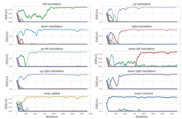
3.14 Training of the experts. . . 66
3.15 The output of the experts can be labelled by a standard MNIST classifier. . . 67
3.16 The experts generalise to new, unseen datasets. . . 67
3.17 The experts can be applied sequentially. . . 69
4.1 Summary of the few-shot learning task. . . 74
4.2 Summary of the few-shot learning pipeline. . . 79
4.3 t-SNE embeddings for the last layer weights of CIFAR-100 andminiImageNet. 80 4.4 Model comparison on CIFAR-100. . . 92
4.5 Results onminiImageNet with different network architectures. . . 95
4.6 Comparison of neural network architectures and training set sizes. . . 96
4.7 Choice of the regularisation constant for logistic regression on few-shot learning. 98 4.8 Online learning with ResNet-34 features. . . 98
5.1 Static entities, proxy variable and projections. . . 102
5.2 Proxy variable and projection in images. . . 105
5.3 Re-ordering shuffled video frames using proxy variables. . . 108
5.4 Results of the NLP experiment. . . 113
3.1 Taxonomy for DG and MTL. . . 21
3.2 Methods used in the numerical experiments for DG. . . 45
3.3 Methods used in the numerical experiments for MTL. . . 59
4.1 Inference during the concept learning phase. . . 90
4.2 Inference during the few-shot learning phase. . . 90
4.3 Likelihood of the weights under different models. . . 91
4.4 Results onminiImageNet. . . 96
5.1 Results in detecting the causal direction in image pairs. . . 107
A.1 Neural network architectures for the competition of experts. . . 133
B.1 Training classes forminiImageNet. . . 138
B.2 Validation classes for miniImageNet. . . 139
B.3 Test classes for miniImageNet. . . 139
B.4 Network architecture for the ResNet-34. . . 140
Abbreviations
DAG Directed Acyclic Graph.
SEM Structural equation model.
OCD Observational Causal Discovery.
ANM Additive noise model.
DS Dataset shift.
CS Covariate shift.
MMD Maximum Mean Discrepancy.
DG Domain Generalisation.
MTL Multi-task Learning.
CNN Convolutional Neural Network.
MAP Maximum A Posteriori.
RKHS Reproducing Kernel Hilbert Space.
GAN Generative Adversarial Network.
GMM Gaussian Mixture Model.
General notations
Rd ddimensional real vector space.
R+ Non-negative real numbers.
X Set.
Probability
X Real valued random variable.
X Vector valued random variable.
P(X) Probability distribution of random variableX. p:=p(X) Probability density function of random variable X.
µκ(P) Mean embedding of distributionP in the RKHS defined by kernel
κ.
d
= Equality in distribution.
Statistics
i.i.d. Independent and identically distributed.
{xi}ni=1 iid
Introduction
Machine learning provides tools for making predictions in the world around us. When learning with supervision, a machine or agent is given a training dataset of input-output pairs (x, y), where x ∈ X is a feature representation of the data point, and y the output
value corresponding to the inputx. The goal of the agent is to build amodel M allowing
us to make predictions on new test data pointsxe. It remains nonetheless unclear where the new data point xe is coming from, and whether M can be used for prediction without further modifications. Most standard approaches for supervised learning assume that the test data is drawn from the same distribution P as the training data, thus circumventing this problem:
when testing on data coming fromP,M may be deployed directly.
In practice, however, this assumption is often violated for a variety of reasons. The test data may have been acquired on a subset of the population which is not well represented in the training set. The labels present in the test set may be different from those abundant in the training set. A robot having learned to play tennis well should in principle be able to transfer knowledge to sports sharing some of the same skills, such as squash. In all these situations and many more, we wish to learn models which can be transferred to the test distribution.
A fundamental problem when learning a predictive model M is to learn a feature
representation
h:X →Xe
of the input data which better expresses the key attributes of the input necessary to solve the task at hand. In standard multi-class image classification, the input to the model is usually a vector of pixel intensitiesx∈Rd from which distinguishing labels is a difficult task. From the machine’s perspective, xis a vector of numbers with little apparent regularity. Simply rotating the image leaves the output trivially recognisable for humans, yet the resulting pixel intensities look very different from the original x. Powerful machine learning models such as kernel methods (Schölkopf et al., 2002) and deep neural networks (Goodfellow et al., 2016)
build a linear model on top of a learned feature representations h(x), providing evidence that it is possible to learn informative features leading to high classification accuracy with linear models. One can understand, for instance, that a binary vector where each dimension indicates if an attribute is present in the image (Is there a tail? Is there a chair?) is significantly simpler to exploit for classification than the raw pixel representation. This thesis analyses different problems in machine learning in which transfer occurs, and introduces methods for learning appropriate representations and models.
But what kind of assumptions regarding the similarity between different distributions can be made? A main contribution of this thesis is the formulation of regularity assumptions between training and test distributions using ideas from the field of causal inference, see Chapter 3. We motivate that learning representations which exploit causal properties of the data generating process leads to attractive properties for transfer when the training and test distributions shift. One fundamental axis of causality is thinking about how the data came to be, what are the mechanismsunderlying the generation of the data, which in turn explain the statistical dependencies we measure. Exploiting such dependencies provides a powerful tool for prediction under the same training and testing conditions, but can easily break under distribution shift. We argue that onlycausal features of the target variable should be used for prediction when no data from the test task are observed. This is an application of the principle of independence between cause and mechanism (Peters et al., 2017): the function or mechanism transforming causes to effect remains invariant to a change in the distribution of the causes. Such an invariant mechanism mapping causes to effect can thus be re-used for prediction in distributions which are drawn from the same causal graph, even when the statistical properties of such distributions differ. A first objective of this thesis is thus to show that invariant causal features provide a powerful framework to discuss distribution shift problems. We further exploit this principle when a probability distribution P is modified
by several independent functions. This is the case, for instance, when a distribution over natural images is transformed by different noisy processes and geometric transformations. We show that given data from these transformed distributions, we can recover an approximate mapping back to the original distributionP without supervision, and the learned mechanisms
generalise to new distributions altogether. This result further supports the re-usability of models resulting from causal assumptions.
The success of deep learning methods in supervised learning problems requires large amounts of labelled data. Often, as providing labels for a dataset is expensive, only a handful of examples are available and these methods cannot be applied. The problem of few-shot learning receives as input an initial large dataset abundant in labelled data, and a small dataset containing new classes that are not present in the training set. From the perspective of human learning, recognising new entities in the world around us seems to leverage two key properties: first, we extract powerful visual features allowing us to focus on high level attributes of the entities we want to recognise; and second, we are able to transfer information
from similar entities we have encountered in the past. Learning to recognise a new type of flower is made easier when we have seen many types of flowers before and are aware of the features they share, and the ones which differentiate them. Inspired by this observation, we propose to build representations using an initial large dataset with standard deep learning approaches. If the new classes are similar to the training classes, we show empirically that these representations transfer well and allow us to quickly learn new concepts, achieving state-of-the-art results in the miniImageNet dataset. A second goal of this thesis is thus to provide a framework for few-shot learning and motivate that better features for batch classification transfer well to new few-shot learning classes.
Causal discovery algorithms aim to find the causal direction between variables given a sample from their joint distribution. Inferring causality from purely observational data is often not possible, and assumptions about the data generating process must be made for a causal footprint to become identifiable. We present an extension of causal discovery motivated by the following question: how can you teach a machine that the concept “virus”causes the concept “death”? The causal direction is quite clear to us, but is based on an understanding of biological processes, and how untreated infection can lead to death. From the point of view of causal discovery, obtaining a sample from two such static entities x and y which
could be fed to a causal discovery algorithm is an ill-defined problem. Using an additional source of randomness, we propose to build representations of x and y from which we can
infer the causal direction. A third objective of this thesis is thus to show empirically that we can construct representations which transfer the causal footprint existing between the original static entities. We introduce a dataset of human-designed, human-validated pairs of concepts, and show that we can correctly identify over 75% of the causal directions using a causal discovery algorithm.
1.1
Outline and Contributions
We provide an outline of this thesis, as well as the major contributions.
• Chapter 2 provides a brief introduction to causal inference and discovery, and describes key properties which are exploited later in the thesis. In particular, Section 2.3 introduces the idea of invariant causal conditionals, and summarises some results on the identifiability of the causes when data from different tasks are available. These ideas motivate the methods for domain shift introduced in Chapter 3. Section 2.2 introduces observational causal discovery, and methods for estimating the causal direction between two variables given only an observational sample from their joint distribution. These methods are used to identify the causal direction between static entities in Chapter 5. • Chapter 3 focuses on the distribution shift problem. We introduce a relaxation of
the setting in which no data from the test task are observed. We motivate that using onlyinvariant features is optimal when the new task is chosen in an adversarial way. Section 3.2.6 introduces a method for estimating an invariant subset from data. In Section 3.3, we also provide a method to exploit this knowledge for prediction when some data from the test task are observed. Both these scenarios are discussed in Rojas-Carulla et al. (2018). Section 3.4 discusses a specific application of multi-task learning in which we want to identify and invert a set of functions automatically and follows Parascandolo et al. (2018). We show that MNIST digits transformed by a series of geometric and noisy transformations can be mapped back to their canonical counterpart without supervision. We further show that the learned mappings generalise to unseen datasets. • Chapter 4 expands on Bauer et al. (2017). We propose a framework for few-shot
learning based on two insights: using features learned from a large image dataset makes learning at few-shot time significantly easier, and the weights of the network contain information about the classes and can be used to regularise the weight vectors of the new classes. Our probabilistic method achieves state-of-the-art in a standard dataset for few-shot learning, putting into context recent developments in the field arguing for meta-learning methods.
• Chapter 5 focuses on the problem of causal discovery between twostatic entities, and is based on Rojas-Carulla et al. (2017). How do we apply a causal discovery algorithm to discover the relation between a painting and its counterfeit? In such case, only one example of each paining is available, while a key ingredient of causal discovery methods is having access to a large sample from which a causal footprint can be measured. We introduce the notion of proxy variable to build representations of the static entities from which the causal direction can be inferred. To assess the methods, we construct a large dataset of pairs of causal concepts, such as “virus” and “death”.
All the work was done in collaboration with several colleagues, including Jonas Peters, Richard Turner and Bernhard Schölkopf. Chapter 4 is based on equal contribution work with Matthias Bauer, but I did not work on designing and training the neural networks for batch classification. Section 3.4 is based on work to which I contributed in ideas and part of the writing, but not in the implementation.
The papers cited previously are mentioned below.
Rojas-Carulla, M., Schölkopf, B., Turner, R., and Peters, J. (2018). Invariant models for causal transfer learning. Journal of Machine Learning Research
Bauer, M., Rojas-Carulla, M., Świątkowski, J., Schölkopf, B., and Turner, R. (2017). Discriminative k-shot learning using probabilistic models. Bayesian Deep Learning Workshop of the 31st Conference on Neural Information Processing Systems (NIPS)(equal contribution) Parascandolo, G., Kilbertus, N., Rojas-Carulla, M., and Schölkopf, B. (2018). Learning independent causal mechanisms. Proceedings of the 35th International Conference on Machine Learning (ICML), 80:4033 – 4041
Rojas-Carulla, M., Baroni, M., and Lopez-Paz, D. (2017). Causal discovery using proxy variables. Workshop of the International Conference on Learning Representations (ICLR)
During my PhD, I also worked on the following paper but do not discuss it in the thesis. Kilbertus, N., Rojas Carulla, M., Parascandolo, G., Hardt, M., Janzing, D., and Schölkopf, B. (2017). Avoiding discrimination through causal reasoning. In Proceedings of the 31st Conference on Neural Information Processing Systems (NIPS), pages 656 – 666
An Overview of Causal Inference
“I would rather discover a single causal law than be king of Persia”. These words by the Greek philosopher Democritus attest to the long and challenging pursuit led by scientists and philosophers in the field of causality. From a scientific perspective, being able to establish with confidence the causal laws relating variables of interest remains a fundamentally difficult question. It is nonetheless true that the scientific community is more often than not interested in questions of a causal nature. What are the main causes of the obesity epidemic? What is the effect of increasing interest rates on economic growth after a recession? These questions are difficult because they require significantly more understanding of the true underlying mechanisms than traditional predictive modelling. Indeed, performing an action, orintervention, on the system of interest usually changes the distribution of the data, and insights resulting from statistical dependencies previously measured should be carefully revisited. It may be, for instance, that the amount of saturated fat in a person’s diet is highly predictive of obesity. Concluding that saturated fat must be restricted solely on this premise is a significant leap of faith with remarkable public health consequences. While the hypothesis that high saturated fat causes obesity is valid, it is only one of many possible explanations. It may be, for instance, that the amount of saturated fat is simply confounded by total calories consumed, which fully explains obesity. It may also be that sugar is the culprit, and replacing sugar calories for saturated fat calories at constant total calories decreases a person’s weight. In order to test these assumptions, careful large scale experiments must be carried out.
The gold standard for establishing causal links are randomised experiments. Consider the important problem of determining the effect of a new drug on recovery. The ideal experiment would take the same sick patient, clone her, and apply the treatment only to one of the copies. If only the treated individual recovers, the drug is a success. Since this imaginary intervention is not possible, randomised experiments replace this idealised experiment by a large scale experiment on subjects representative of the population in which the drug is to be prescribed. This population is randomly divided into two groups, a control group and an experimental group. The first group is given a placebo (sugar pill) and the second group
the drug under consideration. The randomised aspect of the experiment is essential, as it removes any possible effect of the treatment assignment on recovery (for example, the doctor only assigning the drug to rich people, who recover more often anyway). If the difference in recovery rates between both groups is statistically significant, the effect of the drug is confirmed. It is important to realize that without this experiment, many possible explanations for recovery cannot be ruled out with confidence.
While randomised experiments are a powerful tool for establishing causal links, they are often infeasible for several reasons. A first reason is ethics. A researcher aiming to establish the effect of abortions on some indicator of the woman’s future well-being will certainly never carry out a randomised experiment. A second reason may be the pure impossibility of carrying out an experiment: finding a population of countries willing to have their interest rates tempered with is out of the question. The area of causal discovery emerged from statistics and econometrics to tackle this issue. What can we say about the causal link between quantities of interest based on the available data and the statistical dependencies we measure, without carrying out experiments? Section 2.2 introduces observational causal discovery, which aims to answer this question when the data available is purely observational and i.i.d. The methods discussed are the causal discovery black-boxes used in Chapter 5. Section 2.3 further assumes that some experimental data is available, and introduces the ideas which constitute the backbone of the methods for transfer learning presented in Chapter 3.
2.1
Fundamental Technical Notions
2.1.1 From Statistical to Causal Dependence
Let X = (X1, . . . , Xp) be p random variables. Predictive modelling relies on statistical dependencies, that is, properties of the joint distribution P(X1, . . . , Xp) are exploited for prediction. Given a featuresX and a target variableY we wish to predict fromX, regression models capture this dependency and build a model ˆY = f(X). However, a statistical dependence does not in general allow us to establish the causal relation between the variables in X1, . . . , Xp and Y. Reichenbach (1956) attempted to formalise the relation between dependence and causation:
Principle 1 (Principle of Common Cause) If two random variables X and Y are sta-tistically dependent (X̸⊥Y), then one of the following causal explanations must hold:
i) X causesY (write X →Y), or ii) Y causesX (write X ←Y), or
iii) there exists a random variable Z, such that X ←Z →Y. Such a variable Z is called a confounder.
In the third case, X and Y are conditionally independent givenZ (write X⊥⊥Y |Z). In practice, dependencies can be observed between random variables for different reasons that the ones mentioned in Principle 1, and some examples are given in (Peters et al., 2017, Chapter 1.4). Nonetheless, the implications of Principle 1 are strong when we wish to perform interventions in a system and not only predict, and are in line with the well known warning correlation does not imply causation. As a classic example, consider Messerli (2012), where the authors find a significant correlation betweenX =Chocolate consumption, measured
per capita, andY =Number of Nobel prize winners. A common reaction to this finding
often reads beyond the measured statistical dependency and attributes a causal meaning. In other words, people assume that intervening by eating more chocolate will lead to increased intelligence and thus, a higher probability of one day obtaining a Nobel prize. Even the authors of the paper write “since chocolate consumption has been documented to improve cognitive function, it seems most likely that in a dose-dependent way, chocolate intake provides the abundant fertile ground needed for the sprouting of Nobel laureates. Obviously, these findings are hypothesis-generating only and will have to be tested in a prospective, randomised trial.” This hypothesis, however, seems far fetched and quite unlikely. Principle 1 provides a more likely explanation: there is a confounding variable Z which causes bothX
and Y and explains the measured dependence. Z could be, for instance, a country’s wealth
which partly explains a larger disposable income and better quality education. In the absence of a causal link from X to Y, intervening on the amount of chocolate eaten will have no
effect onY. Similar statements are commonplace in the media and highlight the difference
between observing and doing (Pearl, 2009). We present some tools from the field of causal inference developed to discuss interventions and the resulting distribution shifts.
2.1.2 Directed Acyclic Graphs, Structural Equation Models
The causal relation between the variablesX1, . . . , Xpis often represented by a causal Directed Acyclic Graph (DAG)G. An arrowXi →Xj is present inG if Xi is adirect cause ofXj. A DAG entails acausal factorisation of the joint distribution P(X):
P(X1, . . . , Xp) = p Y
j=1
P(Xj|PAGj), (2.1)
where PAGj is the set of parents of Xj in G. Let us consider a simple example with two random variables X and Y whereX is a cause of Y. Standard statistical analysis does not
a priori prefer any factorisation of the join distribution, since P(X, Y) =P(Y |X)P(X) = P(X|Y)P(Y) are both valid equivalent factorisations. Only the first factorisation, however,
is a causal factorisation as in (2.1), and its modules can easily be interpreted when discussing interventions on X and Y. As a concrete example, assume that X = time from birth
and Y =height, where X is clearly a cause of Y. Given a young subject, a hypothetical
intervention which fast-forwards time and therefore ages her 10 years should also imply an increase in height, just as transporting her back to her baby years will make her smaller. If one could, on the other hand, intervene on height, there is absolutely no reason to expect a movement in time. Despite both interventions being impossible in practice and fantastic in nature, we can reason about them because of our knowledge of the biological mechanism relating age to height.
Independence of cause and mechanism In the factorisationP(X, Y) =P(Y |X)P(X)
in the previous example, the distribution of the cause X isindependent of the conditional
P(Y |X). The opposite, however, does not hold: a change in the distribution P(Y) often
modifiesP(X|Y). This is an instance of the Principle of Independent Mechanisms, which
Peters et al. (2017) define as follows:
Principle 2 (Independent Mechanisms) The causal generative process of a system’s variables is composed of autonomous modules which do not influence each other. In the probabilistic case, this means that the conditional distribution of each variable given its causes does not inform or influence the other conditional distributions.
As mentioned in Peters et al. (2017), this principle is plausible when the conditionals in (2.1) correspond to physical mechanisms in the world. Some attempts to formalize further the notion of independent mechanisms has been proposed in Janzing and Schölkopf (2010) using the notion of Kolmogorov complexity. However, the problem of quantifying independence between mechanisms given data remains an open research question.
Structural equation models The causal relation between random variables can be described by a Structural Equation Model (SEM). Although different definitions exist, we use the one from Peters et al. (2014).
Definition 3 A Structural Equation Model is a tuple (E, P(N)), where E = (E1, . . . , Ep) is a set of p equations:
Ej : Xj =fj(PAGj, Nj), j = 1, . . . , p. (2.2) PN is the joint distribution of the noise variables N, which are assumed to be jointly independent. The vertices of PAj are the parents of Xj in the corresponding DAG G.
Each equation Ej for j ∈ {1, . . . , p} specifies the functional relation between Xj and its parents. Standard methods for learning a causal graph from observational data include conditional independence tests (Zhang et al., 2011) and additive noise models (Peters et al., 2014).
Importantly, the equality in (2.2) should be interpreted as an assignment rather than an algebraic equality: Ej allows us to compute Xj from changes in its parents, but modifying
Xj does not trickle up to its parents inG. In other words, modifying an equation in the SEM has an effect on the distribution of its descendants, but not its parents. This leads us to the definition of interventions.
Definition 4 (Interventions) A hard intervention on Xj consists on settingEj :Xj =x for somex and using the SEM to recompute the value of all the descendants of Xj. Similarly, a soft intervention sets Ej :Xj =Ne for some random variable Ne.
A hard intervention Xj = x is refered in Pearl (2009) as a do operation and is denoted do(Xj =x). Similar notations are proposed for soft interventions.
Simple example. Consider the following simple bivariate example:
X=N1
Y =X+N2,
(2.3) whereN1 andN2 are two independent Gaussians, andN2∼ N(µ, σ2). Then trivially (X, Y) follows a bivariate Gaussian distribution. Given the intervention do(X = 5), X becomes
a point mass distribution and Y ∼ N(µ+ 5, σ2). The joint distribution arising from an
intervention is thus different from theobservational distribution. A fundamental property is that, despite the change in the joint distribution, the conditional P(Y |X=x) remains
the same before and after the invervention. Note, however, that the intervention do(Y = 5)
does not modify the distribution of X due to the asymmetrical assignment in the SEM. The
ability to model interventions is a key property of causal models.
2.2
Observational Causal Discovery
Significant efforts in causality have focused on the problem of observational causal discovery. As discussed in the previous section, the gold standard for establishing causal relations is randomised experiments, which heavily rely on experimentation. In many real world settings, experiments are not feasible for ethical or practical reasons, yet discovering causal relations remains important.
Observational causal discovery (OCD) attempts to establish causal relations from purely observational data. Given a sample Diid∼P(X1, . . . , Xp), OCD methods try to recover the causal graph relating the random variables X1, . . . , Xp. In general, causation cannot be inferred from purely statistical dependence, and assumptions regarding the data generating process must be made for the causal graph to become identifiable from the observational distribution. We present methods for bivariate causal discovery, and leave out a large family of methods focusing on conditional independence properties which often assume that P is
−
1
0
1
X
−
1
0
1
Y
(a)Y =f(X) +ϵ−
1
0
1
Y
−
1
0
1
X
(b)X=g(Y) +η Fig. 2.1 An Additive Noise Model (ANM).application of additive noise models to more than two variables is discussed in Peters et al. (2014).
Bivariate causal discovery aims at differentiating the three scenarios in Principle 1 given a sample {(xi, yi)}ni=1
iid
∼P(X, Y), i.e., we want to decide between X → Y, Y → X or X←Z →Y for some confounding variableZ. We present two families of methods for this
task. They both rely on different assumptions which lead to a measurable causal footprint in the joint distribution.
2.2.1 Additive Noise Models
Additive noise models (Hoyer et al., 2009; Peters et al., 2014), or ANM, assume that in the correct causal direction, the effect is computed as a function of the cause with added independent noise. If we assume that X is a cause of Y, the ANM assumption implies that
there exists a function f such that
Y =f(X) +ϵ,
where ϵ⊥⊥X. The ANM assumption leads to the identifiability of the causal direction if
the converse does not hold, that is, there exists no function gsuch that X=g(Y) +η with η⊥⊥Y. Measuring a dependence between the noise termη and the inputY in the anti-causal
direction is the causalfootprint which renders the causal relationidentifiable from the joint distribution P(X, Y). An example of an identifiable ANM is provided in Figure 2.1. Note
that additive noise models in the bivariate setting aim to distinguish X→Y from Y →X
and do not consider the confounded case.
Example of non-identifiability The follow example is borrowed from Peters et al. (2014). Consider that the relation betweenX and Y is linear:
Y =βX+ϵ, (2.4)
whereϵ⊥⊥X and bothX and ϵare Gaussian. Then X=βYe +ϵ,e where eϵ ⊥⊥ Y, βe =
βVar(X)
β2Var(X)+Var(ϵ) and eϵ = X−βYb . The existence of a mapping with independent noise terms in both directions makes linear relations with Gaussian noise non-identifiable. Nonetheless, Peters et al. (2014) show that (2.4) becomes identifiable if the noise variableϵis non-Gaussian, meaning that there exists no (β,e
e
ϵ) such thatX =βYe + e
ϵ with
e
ϵ ⊥⊥ Y. Moreover, they provide further conditions for the identifiability of additive noise
models in the non-linear setting.
2.2.2 Training Based Methods
Often, the ANM assumptions are violated. For instance, the noise may be multiplicative or heteroskedastic. Methods such as the randomised Causation Coefficient (RCC) (Lopez-Paz et al., 2015) proceed by first training a classifier to predict the causal direction given as input a sample from the joint distribution. RCC assumes that a training set D={(Si, li)}ni=1 is available, where Si = {(xij, yji)}
ni j=1
iid
∼Pi(Xi, Yi) is a sample from a distributionPi(Xi, Yi),
li = 1 ifXi →Yi andli =−1 ifYi→Xi. These training pairs can be simulated by generating generic causal pairs or using real data. RCC creates a feature representation of each sample
Si using kernel mean embeddings (Smola et al., 2007), and learns a binary classifier usingD to identify the causal footprints necessary to classify samples from new distributions.
At test time, a sample{(xi, yi)}ni=1 iid
∼P(X, Y) is given to RCC for prediction. One may
add a third class to the training data to allow for the confounded case. Similar methods include the Neural Causation Coefficient (Lopez-Paz et al., 2017), which computes features forSi using a neural network instead of kernel mean embeddings.
2.3
Causal Inference Using Invariant Predictions
The previous sections presented two families of methods and assumptions which make the DAG identifiable from observational data. This section presents the approach from Peters et al. (2016) which relies on invariance properties verified by causal variables when experimental
data from several “tasks” is available. The ideas presented are related to the assumption of independence of cause and mechanisms (Janzing and Schölkopf, 2010; Schölkopf et al., 2012) and exogeneity (Zhang et al., 2015). These ideas motivate the approach for handling distribution shift presented in Chapter 3.
Let Y ∈Rbe a variable we wish to predict from features X= (X1, . . . , Xp). Moreover, Ddifferenttasks, denoted as environments in Peters et al. (2016), are available at training time and we denote by (Xk, Yk) the feature and target variables in task k∈ {1, . . . , D}. In
the context of causal inference, these tasks may correspond to different interventions on the
p features (but not on the target variable), or to different experimental settings in which the
data was collected. We focus on linear SEMs with additive noise, but Peters et al. (2016) present an extension to the non-linear case. Peters et al. (2016) assume that the Dtasks are
related as follows:
Assumption 5 There exists a vectorγ∗∈Rp of linear causal coefficients such that:
∀k∈ {1, . . . , D}, Yk=µ+ (γ∗)tXk+ϵ, ϵ∼Pϵ, (2.5)
where ϵ has zero mean and finite variance. Let S ={u : γ∗u ̸= 0} and assume that XS is independent of ϵ.
The variables XS are called causal predictors. Assuming that the underlying model is truly linear, what are the implications of Assumption 5 and what are its consequences for causal inference? Equation (2.5) is assumed to hold for all Dtasks. In particular, the
distribution of ϵdoes not depend on the task, thus the conditional distribution Yk|XkS is invariant across all tasks. The invariance under interventions of SEM relates to the notion of autonomy (Aldrich, 1989) or stability (Pearl, 2009), which state that modifying one equation in the SEM does not affect the remaining equations, or in other words that the equations in a SEM are autonomous. This assumption is realistic if the equations in the SEM are not seen as an algebraic equality but as mechanisms which link a set of causes (the parents in the corresponding DAG) to the value of the corresponding effect variable.
Peters et al. (2016) analyses the question of identifiability of the true causal parents of a target variable Y given multiple tasks for which Assumption 5 holds. In particular, given a
set of interventionsk∈ {1, . . . , D}they define the set of identifiable causal predictors, which
is proven to be a subset of the true causal predictors as defined in Assumption 5. Moreover, the number of identifiable coefficients grows as Dincreases, that is, observing more tasks
leads to better estimation of the true causal parents. For linear SEMs with Gaussian noise, Theorem 2 in Peters et al. (2016) provides sufficient conditions for the identifiability of the true causal predictors. They also propose two algorithmic approaches to build confidence intervals on the set of identifiable causal predictors.
2.4
Causality in Machine Learning
At first sight, it is unclear how causality can be useful in standard machine learning. Standard learning theory assumes that in a supervised learning problem, the training and test data are i.i.d. draws from the same distributionP(X, Y) over features and target. This testing setting
does not require knowledge of the causal structure relating the variables under consideration, as statistical dependence is sufficient for learning the optimal predictor in the population case.
We claim that causality can be useful for machine learning when discussing non i.i.d. problems, such as transfer learning and reinforcement learning, or when interpretability of the features is a requirement. This thesis presents in Chapter 3 a method for distribution shift inspired by invariance properties introduced in this chapter.
Reinforcement learning provides an intriguing test bed for causal assumptions. It is well known that agents trained to play games using model free reinforcement learning do not generalise when something as simple as the background of the game changes (Diuk et al., 2008; Kansky et al., 2017). In part, this is probably partly due to a training protocol which relies only on statistical dependencies to learn policies, and not on learning invariants of the environment. A framework for reinforcement learning inspired by causality would rather encourage learning a model of the world and understanding which modules are re-usable in different scenarios. For a robot interacting with the world, learning invariant properties of how objects react to physical laws and interactions with the robot should be of high importance for generalising to new environments.
Causality can also contribute to problems where understanding decisions and features is important. Often, we are not only interested in a prediction or a decision, but in why this decision was made. This can be due to a variety of reasons, including regulatory constraints, moral requirements or simply a desire for deeper understanding of the systems under study. Causality has also been applied as a tool for thinking about fairness and discrimination in automatic decision systems (Kilbertus et al., 2017).
More broadly, understanding and discovering causal laws is a key element in the develop-ment of machine intelligence and reasoning.
Invariant Causal Representations
for Transfer Under Distribution
Shift
Standard machine learning assumes that the training and test data are drawn from the same distribution. Problems in which the test distribution differs are nonetheless ubiquitous in practice, a phenomenon we refer to as distribution shift. Building a music recommendation algorithm uses large amounts of data from a database of users, but not from a user new to the service, whose taste is unique. Data may also be gathered using different instruments or sources. In an image classification problem, the new test images may have been clicked with a new camera. In language, an algorithm may be trained with large amounts of text data coming from a large source such as Wikipedia, different from the language that will be given as input by the end users. The context of the examples may also shift: animals in an image training set may be depicted mostly in broad daylight, while the test set contains shots taken in the evening. Algorithms for distribution shift aim to address this mismatch between training and test distribution. A formal statement, as well as some of the standard methods and assumptions for distribution shift, are introduced in Section 3.1.
The goal of this chapter is to build representations of the data which transfer when the distributions shift. We introduce a new assumption for two specific modalities of domain shift of increasing difficulty: multi-task learning, where data from the test task are observed (Section 3.3), and domain generalisation, where no data from the test task are available (Section 3.2). This terminology is arguably not standard, but will be kept consistent throughout this chapter. In Baxter (2000) and several references therein, domain generalisation is referred to as learning to learn. For transfer to be possible, assumptions on how the training and test distributions are related must be made. We motivate that representations of the data for these challenging settings can be built on top of assumptions
motivated by causality. In particular, the notions of causal graph andinterventionintroduced in Chapter 2 may be used to relate the training and test tasks: the same causal graph may describe the generative process of the data in the different tasks, and each task corresponds to different set of interventions on this graph. Under these assumptions, we show that the feature mapping which simply selects a subset of causal features has attractive properties for domain generalisation and multi-task learning. Importantly, these transferable representations may have arbitrarily different distributions between tasks, yet the function ormechanism mapping them to the target variable is preserved, as motivated by Principle 2 in Chapter 2.
Finally, Section 3.4 focuses on a specific application of multi-task learning in which each task is computed by transforming a canonical distribution P via some mechanisms. In the motivating example, the canonical distributionP is the standard MNIST distribution,
and the different mechanisms are simple transformations of these canonical digits such as translation or noise addition. The main motivation is that understanding how the new representations relate to the canonical distribution leads to re-usability: for instance, having trained a classifier onP using labelled data, we wish to use it on the transformed digits as
well without gathering new labelled data. We provide an algorithm that learns approximate mappings from the transformed examples back to their canonical counterpart without labelled information. The transformed examples can be labelled by a classifier trained on the canonical distributionP. Importantly, we find empirically that the learned inverse mappings generalise
to data from a new, unseen distribution, further enhancing their modularity and re-usability. Both our contributions in domain generalisation and multi-task learning motivate the idea that representations and models satisfying causal invariance properties are robust with respect to changes in the statistical properties of a probability distribution.
3.1
An Overview of Distribution Shift
3.1.1 From Standard Machine Learning to Distribution Shift
The standard framework for supervised machine learning assumes that a dataset D = {(xi, yi)}ni=1
iid
∼P(X, Y) drawn i.i.d. from a probability distribution P(X, Y) on X × Y is
available. The goal is to useD to build a model capable of predicting thetarget variable Y
givenfeatures X. Both regression and classification fall within this paradigm. Underlying this process lies the motivation that this model will perform well on new instances{xi}mi=1
iid
∼P(X) for which the target variable needs to be predicted. In practice, it is most often assumed that the model will be tested on data drawn from the same distributionP(X, Y). This assumption
is nonetheless strong and is often violated, which leads to adistribution shift.
Definition 6 (Distribution shift) A learning problem suffers from distribution shift if the test data is drawn from a distribution PT different from the training distribution P.
Spam detectors, for instance, are trained on emails from users which receive attacks of a different nature than those experience by the end user. Even in problems typically associated with the i.i.d. paradigm such as image detection the risk of dataset shift exists: if the training images only contain dogs mostly resting in their bed, the model may perform arbitrarily bad given a dog playing outside.
We first present some key ideas from the standard i.i.d. prediction setting. We then introduce a framework for dataset shift introduced in Baxter (2000).
3.1.1.1 Overview of Standard Supervised Learning
The goal of standard supervised learning is to predict a target variable of interestY ∈ Y
given features X ∈ X. Let P(X, Y) be the corresponding joint distribution. In order to
move forward, we require both a measure of the gap between the predictions and the target, and a specified set of functions to which we restrict our model. We measure how good our predictions are using a loss function ℓ:Y × Y →R+. Moreover, we restrict our model to a hypothesis class denotedH. H may correspond, for example, to the set of linear models in Rd, or the class of functions induced by a neural network with a fixed architecture.
During learning, our goal is to learn a modelh∗ ∈ H which minimises the expected loss
or risk:
RP(h) =EX,Y [ℓ(h(X), Y)]. (3.1) In reality, we do not have access to the true data distributionP, but observe a sample
{(xi, yi)}ni=1 iid
∼P(X, Y). Empirical risk minimisation (Vapnik, 1992) minimises instead the
empirical risk, defined as
b RP(h) = 1 n n X i=1 ℓ(h(xi), yi).
A fundamental question which has interested practitioners and theorists alike is knowing how large the available sample from P must be to guarantee good performance, or generalisa-tion, onunseen data pointsdrawn i.i.d. from P. From a theoretical perspective, this question
is well understood, and the convergence of the empirical risk to the true expected risk is governed by the VC dimension of the hypothesis classH, see (Blumer et al., 1989; Vapnik,
1982) for convergence bounds and finite sample guarantees. The complexity of the hypothesis class Hplays a fundamental role in machine learning, as there is a trade-off between between
the bias and variance of the functions in the hypothesis class (Geman et al., 1992). Intuitively, if the function class allows for too much freedom, a small empirical error may be achieved on the training data at the expense of poor generalisation . Too poor a model class, however, leads to poor predictive performance.
Empirical risk minimisation does not deal with the common scenario in which the test data is drawn from a distribution which differs from the training distribution. The following section extends the previous setup to this important scenario.
3.1.1.2 Extension to the Multiple Task Problem
LetP be a set of joint probability distributionsP(X, Y) onX × Y andMa distribution over P.1 P may consist on a finite ordered set of probability distributionsP = (P1, . . . , PD), and
Mdraws an index in{1, . . . , D}according to some distribution and returns the corresponding
P.
Moreover, define a family of hypothesis H such that each H ∈H is a set of functions
h:X → Y, similarly to the hypothesis classes in the previous section.
Definition 7 We say that P ∈ P is a task2, and M is a distribution over tasks.
Given a non-negative loss function ℓ : X × Y → R+, our goal is to find a family of hypothesisH∗ which minimises the following expected risk over distributions drawn from M:
RM(H) =EP∼M
inf
h∈HRP(h)
This problem is referred to in Baxter (2000) as thebias learning problem, orlearning to learn (Thrun and Pratt, 1998). The bias learner aims to find a hypothesis class, and not only a function, which contains a good solution for tasks drawn according to M, and is closely
related to meta-learning (see for instance Lemke et al. (2015)).
Similarly to empirical risk minimisation, we do not have access to the true distribution over tasksM. Hence, we are given a sample of tasks {Pk}D
k=1 iid
∼ M and for each k∈ {1, . . . , D},
a sample {(xki, yki)}nk i=1
iid
∼Pk. As a proxy of the true expected risk, one may minimise the
empirical riskRbM(H) = 1 D
PD
k=1infh∈HRbPk(h). Uniform convergence results of RbM(H) to
RM(H) are established in Baxter (2000).
Learning theory in the i.i.d. setting analyses how many examples drawn from P need to
be seen during training in order for the solutionh∗ ∈ Hto generalise well to unseen examples
drawn from the same distributionP. In the multi-task setting, the main goal is no longer
to perform well in one specific task, but rather in any task drawn from M. The following
question becomes central for transfer learning in general, and remains a major challenge for the machine learning community:
In the multiple task problem, how many tasks need to be observed in order to achieve good generalisation performance for unseen tasks? Under which assumptions can such transfer take place?
1
See (Baxter, 2000) for a more rigorous mathematical description ofM.
2
In this work, we use the term task and domain interchangeably. Many authors make a distinction between the two, see Pan and Yang (2010), but the distinction is not essential.
method training data from test domain Domain generalisation (DG) (X1, Y1), . . . ,(XD, YD) T :=D+ 1 (X1, Y1), . . . ,(XD, YD), e XD+1 Multi-Task Learning (MTL) (X1, Y1), . . . ,(XD, YD) T=1,. . . ,D (X1, Y1), . . . ,(XD, YD), e X1, . . . , e XD
Table 3.1 Taxonomy for domain generalisation (DG) and multi-task learning (MTL). Each problem can either be used without (first line) or with (second line) additional unlabelled data.
Knowing which knowledge from other tasks can be used when observing a new task seems particularly important. For instance, if all the tasks are completely unrelated, knowledge transfer can be expected to fail, or even hurt performance, see for instance (Ben-David et al., 2010; Rosenstein et al., 2005). As an illustration, consider standard image classification in which the goal is to predict an image label from pixel features. If the tasks consist on a large variety of images, taken from diverse cameras and in a representative set of backgrounds, the availability of multiple tasks should make it easier to find features which are predictive of a given label, and not simply correlated in a given dataset. On the other extreme, consider a binary classification dataset drawn from an arbitrary distribution P, and consider the
distribution Qwhich has identical support toP but simply flips the labels. While each task
may be easy to solve independently, treating them together makes the problem significantly harder, as it gets close to random guessing.
Setup. During training, we observe D probability distributions P1, . . . , PD referred to
as training tasks. Moreover, a sample{(xki, yki)}iid∼Pk from each training task is available.
We define two different transfer learning problems depending on the nature of the test distributionPT. Domain generalisation (DG) models are tested on a dataset drawn from a
new distributionPT =PD+1 which is not included in the training tasks. DG is a challenging
problem and assumptions regarding the similarity between tasks must be made for learning to be possible. Multi-task learning (MTL) tests on unseen data drawn from one or several of the training tasks. In this case, the goal is to exploit similarities between the training tasks and perform better than learning each task independently. Both DG and MTL can get access to unlabelled data from the test task during training. Table 3.1 presents a summary taxonomy of DG and MTL.
The field of transfer learning considers a wider range of settings we do not discuss. These include, among others, domain adaptation and learning to learn, see Pan and Yang (2010) and references therein for further details.
We have mentioned that the distributions change between training and test, but have not presented methods for measuring the difference between distributions given data. The
following section provides tools for measuring distances between probability distributions. While certainly not exhaustive, the presented methods are essential components of the DG procedures introduced in Section 3.2.
3.1.2 Measuring Differences Between Distributions
We are studying problems in whichdistinct probability distributions are available. Since in practice we do not have access to the probability distributions themselves, we require a method to assess the distance between two probability distributions P and Qbased on two samples
{xi}ni=1 iid
∼P and {yi}mi=1 iid
∼Q. In particular, we wish to perform a two sample test, which tests the null hypothesis H0 : P =Q given the two samples. First, we introduce Levene’s test for equality of variances (Levene, 1960), which tests for equality of the variances of several distributions given only samples. We then introduce the Maximum Mean Discrepancy (MMD) and a kernel two sample test. Finally, we propose a novel method for testing whether
Dscalar samples are drawn from the same distribution, which becomes a key component of
the method introduced in Section 3.2. This is certainly not an exhaustive list, and such tests are ubiquitous in machine learning. Two sample tests are particularly relevant for adversarial generative models (Goodfellow et al., 2014), as the generative component of the network is trying to fool a discriminator, which is essentially performing a two sample test between the real data and the fake data generated by the model. This idea was already used for estimating unnormalised parametric models with Noise Contrastive Estimation (Gutmann and Hyvärinen, 2010). More recently, Lopez-Paz and Oquab (2016) introduce a two sample test by training a binary classifier to discriminate between the two distributions.
3.1.2.1 Levene’s Test For Equality of Variances
Let P and Q be two real valued probability distributions. Two samples {xi}ni=1 iid
∼P and
{yi}mi=1 iid
∼Q are available. Let x = n1 Pni=1xi andy = m1 Pmi=1yi be the empirical mean of both samples. Letui=|xi−x|andvi =|yi−y|, and denote byuandvfor the corresponding averages. Finally, denote by z the overall average n+1mPni=1ui+Pmj=1vi
. We define the test statistic z as
z= (n+m−2)Pn n(u−z) +m(v−z)
i=1(ui−u) +Pmi=1(vi−v)
,
and we test the null hypothesisH0 : Var(P) = Var(Q). UnderH0, zfollows an F-distribution
F(1, n+m−2). The test rejects H0 at levelα ifz > Fα,1,n+m−2, whereFα,1,n+m−2 is the upper critical value of the corresponding F distribution at levelα.
For our purposes, Levene’s test is relevant when both distributions are Gaussian. If we assume they both have zero mean, their variance completely determines the distribution, and the test can be used as a two sample test. The test introduced in Levene (1960) is more
general, as it can be applied to test the variances of the variance of D distributions. We
restricted the exposition to two distributions for clarity. 3.1.2.2 Kernel Two Sample Tests
Kernel methods provide an intuitive, theoretically grounded approach for non-linear machine learning (Schölkopf et al., 2002). One of the most appealing properties of kernel methods is that they render some linear methods non-linear by use of the kernel trick. A function
κ:X × X →Ris called a positive definite kernel if for all n∈N, for all x1, . . . , xn∈ X and
c1, . . . , cn∈R, n X i=1 n X j=1
cicjκ(xi, xj)≥0. A positive definite kernel is associated to a unique Hilbert space H called Reproducing Kernel Hilbert Space (RKHS) with dot product⟨. , .⟩.
There exists a feature mapϕ:X → H such that for any twox, y∈ X, ⟨ϕ(x), ϕ(y)⟩=κ(x, y).
The previous property lies at the heart of kernel methods: the feature representation of a data pointx∈ X implied by the kernel κ isϕ(x), which lives in a potentially infinite dimensional
space. If the algorithm only depends on dot products in the input space, it can often be written in terms of the dot product in the RKHS, and the feature maps do not need to be computed explicitly. This convenient trick is denoted the kernel trick and is at the core of techniques such as non-linear support vector machines (e.g., Schölkopf et al. (2002)).
Recent efforts aim to extend the embedding of datapoints x∈ X to an RKHS to embed
whole probability distributionsP, see Sriperumbudur et al. (2010) and references therein.
Given a probability distribution P and a positive definite kernel κ, we define the mean embedding of P as
µκ(P) =EX∼P [ϕ(X)].
µκ(P) is such that for any function f ∈ H, ⟨f, µκ(P)⟩ = EX∼P[f(X)], so computing expectations with respect to P becomes a linear operation in the RKHS.
But how can we use these mean embeddings to measure the distance between distributions? Gretton et al. (2012) propose a two sample test based on this idea. If a kernelκischaracteristic (such as the square exponential kernel with length scale σ: κ(x, y) = exp (∥x−y∥2/2σ2)), the mean embedding is an injective mapping (Sriperumbudur et al., 2010). In other words, given two probability distributionsP and Q,µκ(P) =µκ(Q) if and only ifP =Q.
Define the Maximum Mean Discrepancy (MMD) of distributions P and Q given a set
of functions F as MMD(F, P, Q) = supf∈F(EX∼P