No. 2011-042
AMBIGUITY AND VOLATILITY: ASSET PRICING
IMPLICATIONS
By Beatrice Pataracchia
April, 2011
Ambiguity and Volatility: Asset Pricing
Implications
Beatrice Pataracchia
Tilburg UniversityAbstract
Using a simple dynamic consumption-based asset pricing model, this paper explores the implications of a representative investor with smooth ambiguity averse preferences [Klibano¤, Marinacci and Mukerji, Econo-metrica (2005)] and provides a comparative analysis of risk aversion and ambiguity aversion. The perception of ambiguity is described by a hidden Markovian consumption growth process. The hidden states di¤er both for the mean and the volatility. We show that the ambiguity-averse investor downweights high-mean states in favor of low-mean ones. However, such distortion appears much stronger in low-volatility regimes: high volatility attenuates the distortion due to ambiguity concerns. It follows that (i) am-biguity aversion always implies higher equity premia but sustained levels of ambiguity aversion do not help explaining the high volatility of the equity premium observed in the data (volatility puzzle); (ii) our calibrated model can match the moments of the equity premium and risk free rate and can generate asset-price stylized facts like a procyclical price-dividend ratio and countercyclical conditional equity premia; however, (iii) high levels of ambiguity aversion, necessary to explain high equity returns, produce counterfactual price-dividend ratio time series across volatility states.
Keywords: Ambiguity aversion, volatility, asset pricing puzzles, ro-bustness.
JEL: D81, E44, G12
1
Introduction
In this paper we examine a standard dynamics asset pricing model in which the endowment law of motion is modelled as a hidden regime switching process and the representative agent learns the probabilities of each state via Bayes rule. We depart from rational expectations assuming that the investor feels
ambiguous about the probabilities of the realization of each state, which di¤er both for the mean and the volatility values. Her preferences are represented
I thank Anja De Waegenaere, Luigi Luini, Bertrand Melenberg, Damjan Pfajfar, Giulio Zanella and seminar participants at the NAKE research day, at the Tilburg University and at the University of Siena for helpful comments and suggestions. Email: [email protected].
by a generalized recursive smooth ambiguity model proposed in Klibano¤ et al. (2005, 2008), which nests the standard Epstein and Zin preferences framework and the maxmin expected utility framework of Gilboa and Schmeidler (1989) as two special cases, respectively with no and maximal ambiguity aversion. Smooth ambiguity aversion is manifested through a pessimistic distortion of the pricing kernel in the sense that the agent attaches more weight to the states with lower continuation values. In this respect, this approach is more ‡exible than the maxmin approach according to which the decision maker conditions her decisions exclusively on the worst case model. The pessimistic distortion implied by the ambiguity-averse preferences suggests that such formalization can potentially contribute to the resolution of the equity premium puzzle (Mehra
and Prescott, 1985). Knight (1921) has been the …rst to distinguish amongrisk
and uncertainty. In this sense, the theory of subjective probabilities nulli…es this distinction by reducing all uncertainty to risk through the use of beliefs expressible as probabilities. In our case, ambiguity aversion on the plausible probability distributions posterior implies that the posterior of the hidden state and the conditional distribution of the consumption process cannot be reduced to a compound predictive distribution, unlike the standard Bayesian framework. The experimental motivation of such preferences modeling is provided by the well known Ellsberg paradox (Ellsberg, 1961), showing that decision makers prefer the risky urn to the ambiguous urn, in a way that violates the expected utility framework.
The goal of our work is understanding and assessing the extents to which ambiguity averse preferences can help explaining the main asset pricing puz-zles: the risk free rate puzzle (Weil, 1989), the volatility puzzle (Shiller, 1981) together with the equity premium puzzle. Furthermore, we also assess the ca-pacity of the ambiguity-averse preferences to imply procyclical price-dividend ratios and countercyclical conditional expected equity premia documented in the literature (e.g. Campbell and Shiller, 1988). Finally, we compare the time series of the price-dividend ratios and the equity premia implied by the model with the observed one. Our attention is focused on the ability of the model to capture the striking increase in prices observed during the great moderation period. Figure 1 and …gure 2 depict, respectively, the post-war time series of the consumption growth rate and the CRSP Value-Weighted price-dividend ratios. They suggest a quite evident negative correlation between consumption volatil-ity and the price-dividend ratios, documented also in Lettau et al. (2008) and Bansal and Yaron (2004). We do not ask ourselves the causes of the decline of volatility, rather we want to investigate its e¤ects on prices and the role of am-biguity aversion in this respect. In order to capture the switching in volatility, we model the consumption growth rate as a hidden Markov switching process with two hidden Markov chains, each of them determining, respectively, the switching between mean regimes and volatility regimes.
We show that the ambiguity-averse investor downweights high-mean states in favour of low-mean ones. However, such distortion appears much stronger in low-volatility regimes. Between two high-mean states, the ambiguity-averse investor removes more mass probability from the best state (high mean and
low volatility) rather than from the high-mean and high-volatility case. Simi-larly, between two low mean states, the distortion downweights more the highly volatile states’ probabilities rather than the stable states’ probabilities. The intuition is the following: when the investor perceives a high-mean observation, the worst case is to think that the quality of the observation is quite bad. Con-versely, after a low-mean observation, the ambiguity averse investor will add mass probability to the low-volatility case since a good quality new is the worst
case1. In other words, ambiguity aversion has a …rst order e¤ect among mean
states. The distortion among volatility states is a second order e¤ect. It fol-lows that (i) ambiguity aversion always implies higher equity premia but (ii) the slighter distortion which results in high volatility times implies a moderation in the price volatility and, overall, an uncertain e¤ect of ambiguity aversion on volatility of returns and prices occurs; (iii) our calibrated model can match the moments of the equity premium and risk free rate and can generate asset-price stylized facts like a procyclical price-dividend ratio and countercyclical condi-tional equity premia; however, (iv) high levels of ambiguity aversion, necessary to explain high equity returns, produce counterfactual price-dividend ratio time series across volatility states.
Ambiguity concerns have recently received a huge popularity in the macro-economic and …nance literature. Contributions have been mainly focused on the maxmin expected utility (or multiple priors) model of Gilboa and Schmei-dler (1989) and the robustness theory developed by Hansen and Sargent (2001, 2008). In the maxmin framework, there exist several papers which consider the e¤ect of ambiguity concerns in asset pricing. Epstein and Schneider (2008) an-alyze the e¤ects of ambiguous quality of intangible informarion on asset prices, Leippold et al. (2008) analyze a learning model under ambiguity in a continuous time framework. This literature is also related to contributions which impose pessimism and beliefs’ distortion in a very speci…c ways without a formalized decision theoretic foundation (Cecchetti et al. 2000, Abel et al., 2002, and Brandt et al., 2004 among others). Our work is closely related to Ju and Miao (2007) who also considers a smooth ambiguity averse investor. However, their work is based on Cecchetti et al. (2000) data set, which ends on 1993, when the decline of consumption volatility was not appreciable yet: the authors do not impose any switching among volatility states and consequently, do not investigate the ability of such preferences to reproduce the negative observed correlaton between consumption volatility and prices.
The paper is structured as follows. Section 2 describes the theoretical frame-work of the smooth ambiguity averse preferences. Section 3 presents the model and the theoretical asset pricing implications. Section 4 provides a comparative analysis of the e¤ects of degree of ambiguity aversion, while Section 5 describes the quantitative implications of the model, both in terms of the analysis of the moments and the time series implications. Section 6 concludes.
1The intuition is similar to Epstein and Schneider (2008) who consider a di¤erent framework where ambiguity is imposed on the quality of the intangible information.
2
Smooth Ambiguity Preferences
Recursive preferences have become a standard tool for studying economic behav-iour in dynamic stochastic environments and for parameterizing risk aversion and intertemporal substitution. We assume that time is discrete, with dates t = 0;1;2; :::At each time t > 0, let fIt:t 0g denote the sequence of
con-ditioning information sets available to an investor at date t: Adapted to this
sequence are consumption processesfCt:t 0g and a corresponding sequence
of continuation values fVt:t 0g associated with this consumption process.
The datetcomponentsCtandVtare restricted to be in the datetconditioning
information set. The continuation values are determined recursively and used to rank alternative consumption processes.
As a starting point, we use Epstein and Zin (1989) recursive preferences, which separate between risk aversion and the elasticity of intertemporal substi-tution such that consumers are not indi¤erent to the timing of the resolution of uncertainty. We use the following constant elasticity of substitution - CES recursion: Vt=H(Ct;[Rt(Vt+1)]) = h (1 ) (Ct)1 + Rt(Vt+1)1 i 1 1 ; (1)
where H is a time aggregator and Rt is a certainty equivalent function. The
time aggregator is all that matters in deterministic settings. The rate of time
preferences, 2(0;1)is assumed to be built in and constant and 1 determines
the intertemporal elasticity of subtitution (IES) for deterministic consumption paths. Following Epstein and Zin, many recent applications, particularly in dy-namic asset pricing models, use the homothetic version of the utility function which combines the constant elasticity time aggregator in (1) with a linear ho-mogenous (constant relative risk aversion) expected utility certainty equivalent:
Rt(Vt+1) = h Et(Vt+1)1 i 1 1 ; (2)
where is the constant Arrow Pratt coe¢ cent for relative risk aversion. When
Vt is convex (concave) in its second argument, that is when > ( < ), the
consumer exibits preference for early (late) resolution of uncertainty.
Considering smooth ambiguity preferences implies considering an additional operator, which will de…ne the certainty equivalent for future utilities taking into account ambiguity concerns. As in Hansen and Sargent (2006, 2007), we impose ambiguity over the transition probabilities of the hidden states. The authors propose a log exponential speci…cation, which, in the simple case of two possible hidden states, takes the form:
Ths(R) = log exp Rj = 1 + (1 ) exp Rj = 2 (3) = min 0 b 1 f[Rj = 1 + (logb log )]b+ [Rj = 2 + (log (1 b) log (1 ))] (1 b)g ;
where is an indicator variable for the hidden state, represent the full Bayesian beliefs (or ambiguity neutral probabilities), the parameter is inversely related
to the degree of probabilities misspeci…cation aversion, so that when ! 1,
Ths(V) = V: This operator produces twisted model probabilities, b: it shifts
probabilities towards the model that has the worse value at time t:Following
Klibano¤ (2005), we use an alternative speci…cation. We start the description of smooth ambiguity model by presenting the static setting of a utility function in which a decision maker is ambiguous over consumption:
0 @Z 0 @u 1 0 @Z S u(C)d 1 A 1 Ad 1 A E E u(C);8C:S!R+;
where u is a von Neumann-Morgestern (vN-M) utility function, is a
func-tion which captures ambiguity attitudes, is a subjective prior over the set
of probability measures on S that the decision maker think possible. There
may be subjective uncertainty about what the right probability on S is: is
the decision maker’s subjective prior over , the set of possible probabilities
over S, and therefore measures the subjective relevance of a particular as
the right probability. Letting = u 1;we see that whileucharacterizes risk
aversion, ambiguity aversion is captured by : a concave characterizes
ambi-guity aversion. Notice that, unless is a linear function (ambiguity neutrality),
there is in general no reduction between and :The perception of ambiguity
is characterized by the subjective set of measures while ambiguity aversion is
completely described by the properties of the function .2
In our model, we consider the dynamic version of the smooth ambiguity pref-erences. and we consider a special case of constant relative ambiguity aversion utility:
(x) = x
1
1 ; >0; 6= 1; (4)
where is the ambiguity aversion parameter. Therefore, we consider the
fol-lowing recursion:
Vt=H(C;T (R(Vt+1)));
where the ambiguity operator, in the simple case of two states, takes the form:
2See Klibano¤ et al. (2005) for a detailed discussion of the separation between ambiguity perception (beliefs) and ambiguity aversion (tastes).
T (R) = " (1 ) (R j = 1) 1 1 + (1 ) (R j = 2)1 1 !# 1 1 ; (5)
which can be compared to (3). ConsideringN generic hidden states and
apply-ing the ambiguity operatoroT to (1), the recursive preferences become:
U(ct; EtVt+1) = 8 > < > :(1 )C 1 t + 2 4 8 < : N X j=1 j;t h Ej;t(Vt+1)1 i(1 ) 1 9 = ; 3 5 1 1 9> = > ; 1 1 : (6)
It is easy to see that if = ;(6) reduces to (1) and the investor is ambiguity
neutral. When > the investor displays ambiguity aversion and no reduction
is possible between the state beliefs and the conditional expectations:
3
The Model
3.1
Endowment
We consider a simple Lucas (1978) endowment economy. In order to capture the e¤ect of the switching of volatility regimes, as in Lettau et al. (2008), we model the consumption growth rate process as a hidden Markov swithing model of the form:
yt= log
Ct+1
Ct
=ct+1 ct= ct+1= t+1 + (vt+1)"t+1; (7)
where the variables t+1 andvt+1are two independent two-state Markov chains
with possible values 1 and 2. We suppose that (1) = h > (2) = l and
(1) = h > (2) = l: The driving process "t+1 is a simple i.i.d. standard
normal. The transition probability matrices of the Markov Chains,P andP
are de…ned as follows:
P = phh (1 pll)
(1 phh) pll ; (8)
P = phh (1 pll)
(1 phh) pll ; (9)
where pii represents the probability of remaining in the mean-state i andpii
the probability of remaining on the volatility-state i. Therefore, we consider
a 4 states economy, whose transition matrix can be computed by taking the Kronecker product between the transition matrices, (8) and (9):
where denotes the Kronecker product operator. Consequently, we consider a
Markov chain,Zt; which switches among four states. State1 is represented by
high growth and high volatility [ = h; = h]; state2 is represented by low
growth and high volatility [ = l; = h]; state3 denotes the state with high
growth and low volatility [ = h; = l] and state 4 is the low-growth and
low-volatility case [ = l; = l].
3.2
Learning
Let de…ne the conditional probabilities of a statejwith j;t= Pr (Zt+1=jjIt)
and the vestor of the conditional probabilities t = [ t(1); :::; t(4)]0: Agents
update their posterior beliefs after each observation via Bayes’rule:
t+1=P ( t ft) 10( t ft) B( ct+1; t); (10) whereft= [ft(1); ::; ft(4)] andft(j) = p21 j exp ( ct+1 j) 2 2 2 j is the
den-sity function of the normal distribution with mean j and j, and the operator
represents element by element multiplication.
3.3
Asset pricing Implications
As it is standard in consumption based asset pricing models, the representative
investor chooses to invest a fractionxk of his disposable wealth Wt Ct on a
risky assetk. The agent’s budget constraint is given by
Wt+1= (Wt Ct) (Rw;t+1); (11)
whereRw;t+1 is the gross return on the wealth portfolio between periodt and
t+ 1, which is also the return on the consumption claim. If we suppose that
there areK traded assets, the return on the wealth portfolio,Rw;t+1, is equal
to PKk=1xktRk;t+1 where PKk=1xkt = 1: We solve the investor’s problem by
dynamic programming methods. The state variables of our problem are the level of wealth and beliefs (Wt; t). We guess the following functional form of
the value function:
Vt(Wt; t) =WtG( t); (12)
and we write the Bellman equation that we substitute in (6):
Vt(Wt; t) = max Ct;x 8 > < > :(1 )C 1 t + 2 4 4 X j=1 j;t h Ej;t(Wt+1G( t+1))1 i(1 ) 1 3 5 1 1 9> = > ; 1 1 :
Wt+1 = (Wt Ct)Rw;t+1; t+1 = B( ct+1; t); (13a) Rw;t+1 = K X k=2 xktRk;t+1+ (1 K X k=2 xkt)Rf;t+1; (13b)
where Rf;t+1 is the gross return on riskless asset between periodt and t+ 1.
Substituting the …rst line of the budget constraint we get
V t= max Ct;x 8 > < > :(1 )C 1 t + (Wt Ct)1 2 4 4 X j=1 j;t h Ej;t(Rw;t+1G( t+1))1 i1 1 3 5 1 1 9> = > ; 1 1 : (14)
Proposition 1 The …rst order condition with the respect to consumption plan leads to the following equilibrium condition:
1 = 2 6 4 4 X j=1 j;t Ej;tR 1 1 w;t+1 Ct+1 Ct 1 1 ! 1 1 3 7 5 1 1 : (15)
Proof. See Appendix A.1
Equation (15) can be manipulated in order to emphasize the e¤ects of am-biguous beliefs in the equilibrium determination. Suppose for the moment that our investor is ambiguity neutral. Then the equilibrium condition corresponding to (15) would become 1 = 2 4 4 X j=1 j;tEj;tR 1 1 w;t+1 Ct+1 Ct 1 1 3 5; (16) = " EtR 1 1 w;t+1 Ct+1 Ct 1 1 # :
Let us go back to eq. (15) and let us multiply and divide the expression inside
the square bracket by the termEj;t R
1 1 w;t+1 Ct+1 Ct 1 1 so to get 1 = 2 6 4 4 X j=1 j;t Ej;tR 1 1 w;t+1 Ct+1 Ct 1 1 ! 1 1 1 Ej;tR 1 1 w;t+1 Ct+1 Ct 1 1 ! 3 7 5 1 1 :
We can further multiply and divide the exponent of the square bracket by 11
1 = 1 1 2 6 4 4 X j=1 j;t Ej;tR 1 1 w;t+1 Ct+1 Ct 1 1 ! 1 1 1 Ej;tR 1 1 w;t+1 Ct+1 Ct 1 1 ! 3 7 5 1 1 (17) = 2 6 4 4 X j=1 j;t 1 Ej;tR 1 1 w;t+1 Ct+1 Ct 1 1 ! 1 1 1 Ej;tR 1 1 w;t+1 Ct+1 Ct 1 1 ! 3 7 5 1 1 = 2 4 4 X j=1 ^j;t Ej;tR 1 1 w;t+1 Ct+1 Ct 1 1 !3 5 1 1 ; where ^j;t = j;t 1 Ej;tR 1 1 w;t+1 Ct+1 Ct 1 1 1 1 1
is the distorted belief used by the investor who fears ambiguity over the transition probabilities. Eq. (17), compared to eq. (16) shows how the ambiguous investor behaves as an ambiguity neutral investor with distorted beliefs3.
The …rst order condition with the respect to the trading startegy,xk, permits
us to characterize the pricing kernel for our model.
Proposition 2 The pricing kernel conditioned on statej is given by
Mj;t+1= 1 1 Ct+1 Ct 1 1 R1 w;t+1 " Ej;tR 1 1 w;t+1 Ct+1 Ct 1 1 # 1 1 1 : (18)
Proof. See Appendix A.2
The pricing kernel is also a hidden stochastic variable. Eq. (18) shows that
when = ;we get the usual pricing kernel for time-non separable preferences
without ambiguity concerns, and when we further impose time separability,
= ; we get the standard pricing kernel M = Ct+1
Ct for CES utility
functions. This equation reveals that optimal portfolio rules are a¤ected by ambiguity. The gross risk free rate (or bond return) is given by
1 Rf;t+1 = 4 X j=1 j;t(Ej;tMj;t+1):
3Note, however, that the expected returns, being de…ned via the price-consumption and price-dividend ratios, depend on the degree of ambiguity aversion, in the general case in which utility functions are not logarithmic.
LetPtDdenote the ex-dividend price of a claim to the dividend stream measured
at the end of timet, andPtC denote the ex-dividend price of a share of a claim
to the consumption stream. We conjecture that the price-dividend ratio is given by
PtD='( t)Dt;
and the price-consumption ratio
PtC='C( t)Ct
where'( )and'C(
t)have to be determined. In equilibrium, we have that on
average, the return on equity,Re, is de…ned as follows Re;t+1 PD t+1+Dt+1 PD t = Dt+1 Dt 1 +'( 1;t+1) '( 1;t) : (19)
As in Campbell(1986) and Abel(1999) the dividend on equity,Dt;is modelled
as consumption raised to a power :4
Dt=Ct;
this speci…cation implies that the volatility of dividends is proportional to the volatility of consumption and it is a convenient representation because, while keeping the number state variables limited, allows for higher volatility of the dividend dynamics compared to the consumption process. Substituting in (15) gives 1 = 2 6 4 4 X j=1 j;t 2 4Ej;t 1 +'C( t+1) 'C( t) 1 1 C t+1 Ct 1 3 5 1 1 3 7 5 1 1 : (20)
The equilibrium condition (20) is a functional equation from which we can derive the price-consumption ratio'C( ):Further, substituting (33) into (32),
we derive the equilibrium condition for the price-dividend ratio function. Proposition 3 The price-dividend ratio of a claim to the dividend stream sat-is…es 4 X j=1 j;t Ej;tMj;t+1 (1 +'( t+1)) Dt+1 Dt ='( t): (21)
We solve these functional equations numerically on a grid of values for the state variables t:5
4Abel (1999) shows that this speci…cation is a good approximation to represent leverage equity.
5In the Appendix we describe the functional equations in more details. The Matlab codes and numerical agorithms are available under request.
4
Comparative Analysis
In this section we present a comparative analysis on the behaviour of prices and the equity premium. These types of studies are not new. Veronesi (1999), Cechetti et al. (2000) or Ju and Miao (2007) study equilibrium prices when the endowment is characterized by a hidden growth rate of the consumption process. Prices are analyzed as a function of the high mean state. These studies typically …nd that the equilibrium prices of the asset are an increasing and convex function of the high mean state belief. The intuition is quite straighforward and has been …rst proposed in Veronesi (1999). Suppose we believe we are in the low growth state. When a positive new arrives, the probability of being in a high growth state increases. This causes the investor to expect higher return in the future, to buy more assets increasing, therefore, the price. At the same time, however, the closer is the probability of being in a high growth state to 0.5, the higher the uncertainty of the investitor about which state is realizing. This uncertainty may cause the investor to wait in order to get more information. The price-dividend ratio timidly increases, suggesting that the former e¤ect dominates the latter. Let us consider the other way around. We believe we are in the high growth state and a bad new occurs. Again the e¤ect is twofold. On one side, investors are incentivated to sell the asset, on the other, again, the uncertainty increases, because our belief is now closer to 0.5. Therefore both e¤ects lower the equilibrium prices and the decrease is more accentuated. This fact causes the price-dividend ratio to be a convex function. Similar …ndings have been documented by Ju and Miao (2007) who include also ambiguity with the respect the transition probabilities between high and low growth states. They show that ambiguity does not signi…cantly modify the characteristics of the price dividend ratio, except that it accentuates the curvature, helping to explain the high volatility of asse prices. Also Lettau et al. (2008) document an increasing and convex price dividend ratio.
Figure (3) represents an example of such comparative study. It proposes the log price dividend ratio as function of the beliefs of being in a low volatility state (upper panels) and as a function of the high-mean state belief (lower panels). Horizontally, we di¤erentiate the conditional cases considered (respectively, high and low mean and low and high volatility). The solid line corresponds to the
ambiguity neutrality case ( = = 25), the dashed and dotted line represents
positive levels of ambiguity aversion, respectively = 5and = 10:
We start our discussion focusing on the lower panels, so to be able to make a comparison with existing studies. In all cases considered the price dividend func-tion is increasing and convex. It follows that the model predicts a pro-cyclical price-dividend function, consistently with the empirical observations. Second, we observe that higher levels of ambiguity aversion always imply lower prices since our investor requires higher premium to hold risky and ambiguous asset. Further, comparing the two panels horizontally, the e¤ect of ambiguity aversion appears much stronger in low-volatility regimes: high volatility attenuates the distortion due to ambiguity concerns. In high-volatility states, it becomes more di¢ cult to distinguish high-growth and low-growth regimes from dividend
obser-vations. That is, in high-volatility regimes the investor perceives the increased risk, but his perception of ambiguity is reduced because the worst-case model is not too "far", given some de…ned norms to measure closeness between data gen-erating processes. The panels above also reveals interesting features. As could be expected, a convex and increasing price dividend ratio is also obtained when plotting against the low-volatility state beliefs. However, the curvature is ‡at-ter for higher levels of ambiguity aversion, which, while implying always lower prices, has a stronger e¤ect when the investor believes that the low-valuation state is very likely. This further implies that the volatility of prices is also re-duced, as if the ambiguity-averse investor, being an insuring agent, reacts less to news. In this respect, ambiguity aversion is providing a rationale for price underreaction to news about fundamentals. Indeed, as we move from the belief of the high volatility state to the low-volatility state, the ambiguity averse in-vestor will continue requiring a compensation for holding the ambiguous asset, while risk aversion will play an attenuated role. This is because our investor is pessimistic and the e¤ects of such distortion of beliefs appear much more accen-tuated in low-volatility states where the low-mean state is perceived worse than the low-valuation state with high volatility. The stronger e¤ect of ambiguity aversion in low-volatility cases causes the price-dividend ratio to be much ‡at-ter suggesting that high leveles of ambiguity aversion will not help explaining the high volatility of equity premium observed in the data (volatility puzzle).Our result is in contrast with Ju and Miao (2007) who claim that, in a world where the switching is only allowed among mean states, ambiguity aversion always increases the volatility of equity returns. The authors focus on the early post-war sample (until 1993) which does not allow to appreciate a sensible switching among volatility regimes.
Figure(4) also compares the dynamics of the expected equity premium for di¤erent level of ambiguity. Again, not surprisingly, the equity premium is always higher for higher levels of ambiguity aversion. When the uncertainty about the state is higher, also the ambiguity premium is higher. This is be-cause ambiguity-averse prefences imply a distortion of beliefs towards the lower continuation state injecting pessimism in the economy.
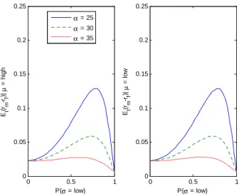
Figure (5) shows that, for given level of ambiguity aversion, uncertainty about volatility state also requires higher expected equity premium. However, increasing ambiguity aversion implies lower levels of equity premium, as if the ambiguity averse investor, not being able to di¤erentiate among worst and best model, perceives less ambiguity. Even if the level of volatility is ambiguous, the ambiguity averse investor is not requiring a compensation for not knowing in which volatile state is the economy. This aspect of the model implies that switching among volatility states does not necessarily imply important e¤ects on prices when the investor is ambiguity averse.
5
Quantitative Analysis
In this section we present the quantitative analysis. Since the state beliefs are the only state variables of the model, we proceed estimating the …ltered state probabilities so to obtain the implied time series of the economic variables of in-terest, prices and equity premia. Our goal is not only engaging in matching the moments, as it is usually done in asset pricing studies, but we want also to com-pare the implied time series with real data and, in particular, we want to assess the ability of the model to replicate long and medium frequency ‡uctuations in prices.
Studies who typically focus on the moments are aimed at explaining …nancial markets’ puzzles like the high equity returns together with very low risk free rates. The observed values are typically very hard to replicate via simple con-sumption based asset pricing models. Further, from Shiller (1981) the literature has also documented very high volatility of the equity returns (see also Camp-bell, 1999 for a survey). Table (1) reproduces sample moments from annual US data. Other important stylized facts emphasized by the literature are the countercyclicality of conditional volatility of stock return, the pro-cyclicality of the price-dividend ratio and the counter-cyclicality of the conditional expected equity premia.
5.1
The Estimated Model
We estimate the model (7)-(8)-(9) byExpectation-Maximation (EM) algorithm.
Estimated coe¢ cients are reproduced in Table (2). The switching between the mean states is more frequent than the switching between volatility states. The persistence of the high growth state is about 7 years, the persistence of a low growth state is almost 5 years, while the persistence of, respectively, the high volatility state and the low volatility state, is 41 years and 27 years. The switch-ing between volatility regimes is a low frequency event and it has been associated to the decline ofmacroeconomic risk, also termedthe great moderation.
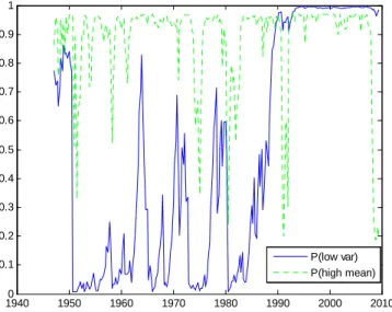
Figure (6) plots the …ltered state probabilities of a low volatility state along with the probabilities of a high mean state. Consumption exhibits a considerable reduction in volatility starting from the 90s and the …ltered state probabilities approach one. The …gure con…rms that the perceived switching among mean states occurs at business cycle frequencies while the switching among volatilities is a low frequency event.
5.2
Matching the Moments
Table (3) refers to the ambiguity neutrality case when we set = 30, such that
the model corresponds to the one calibrated in Lettau et al. (2008) which do not consider ambiguity aversion motives. In our model this case corresponds in
setting = 30 and = 30: Figure (8) compares the observed price dividend
ratios with the one implied by the model and suggests that the calibration considered implies quite low equilibrium prices, therefore, a sustained equity
premium. The risk aversion parameter is, however, much higher than values
typically considered acceptable by macroeconomists ( less than 10 and close
to 2). Next, we consider the role of ambiguity motives ( > ). Tables
(4)-(7) collect the results from simulations for di¤erent values of the discount factor . The tables show di¤erent interesting aspects of ambiguity motives. First, ambiguity aversion always increases the equity return. This is due to pessimistic distortion that ambiguity averse motives place on the investor’s beliefs, so that he requires more compensation to hold a risky asset in an ambiguous economy. Further increasing values of ambiguity aversion lower the risk free rate, helping explaining the equity premium puzzle. On the same time our model is able to generate very low volatility of the riskfree rate together with sustained volatility of the equity returns.
We can also observe that when the risk aversion parameter is quite sustained
(e.g. = 30or = 25) the e¤ect of an increment of the degree of ambiguity
aversion are very moderate. Di¤erent is the case when risk aversion appears
contained (e.g. = 15). In general we can observe that ambiguity aversion
allows matching the mean risk free rate and risky rates with a relatilvely low
value of the risk aversion parameter, like = 10; as it shown by the last rows
of table (7): it is suggested that a value of ambiguity aversion between 20 and 40 could match the moments.
5.3
Time Series Implications
We consider a calibration which is quite satisfactory in matching the moments
described above: = 0:9925; = 15and = 35. As in all calibrations, we set
equal to 1/1.5 and = 4:5:We are interested in understanding the time series
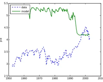
performance of the equilibrium prices and we plot the time series of the price dividend ratio from data with the time series implied by the model. Figure (9) shows that the comparison is not satisfactory. As it has been already observed in the comparative study, the switching from the high-volatility state to the low-volatility state implies a moderation in prices which has not been observed in the data. Extensive simulations show that low values of risk aversion associated with high values of ambiguity aversion imply similar qualitative dynamics. As we already noticed indeed, the e¤ects of ambiguity aversion is much more e¤ective in low volatility states rather than very volatile ones. Therefore, when a very high level of ambiguity aversion is imposed on the investor, the di¤erent intensity of the e¤ect of distortion causes prices to decrease during the last part of the sample. In …gure (10) we compare the observed time series of prices with the
ones implied by our model with equal to25 and ; respectively, equal to25
and35: The …gure makes clear that, while ambiguity aversion is very e¤ective
in lowering the prices explaining, therefore the high equity premium, high levels of ambiguity aversion attenuate the e¤ects of uncertainty on prices in unstable times. Therefore, increased riskiness of the economy attenuates the premium due to ambiguity aversion. This e¤ect worsens the performance of the model
for the last part of the sample, the so called great moderation during which
the respect to mean states reinforces risk aversion, but ambiguity aversion with
the respect to volatility states does not. This tension was never emphasized
previously in the literature and we believe it constitutes an important warning for the growing literature on ambiguity aversion and asset prices.
6
Conclusions
In this paper we consider a smooth abiguity averse representative investor in a standard consumption based asset pricing model. We model consumption and dividend growth rate as a regime switching process. The switching is imposed both on the mean and on the volatility values. We estimate the Markov switch-ing models and show that switchswitch-ing between volatility states is a low frequency event: the …rst part of the postwar sample is characterized by high volatility, while, starting from the 1990s we observe the so calledgreat moderation period. The aim of our study is to understand how ambiguity concerns interact with beliefs about volatility and mean regimes. Our study shows that ambiguity aversion is certainly helpful in order to explain the observed high level of equity premia even with low values of risk aversion. Indeed, higher ambiguity aversion lowers risk free rates while increasing the equity returns. Further, this e¤ect is more accentuated, the lower the level of risk aversion. Not surprisingly, in-deed, ambiguity aversion motives have had a great success on the asset pricing literature in recent years.
However, we also show some additional implications of ambiguity concerns that, up to our knowledge, have not been emphasized previously. We uncover the results summarized in the exercises aimed at matching the moments and we analyze the time series implications of the smooth ambiguity averse preferences. Even if succesful calibrations can match the observed moments of the equity premia and the risk free rate, the implied time series do not appear satisfactory for the levels of ambiguity aversion reqiuired to explain the equity premium puzzle. This is due to the second-order distortion that ambiguity aversion places among volatility states. Indeed, as it has already been widely documented, the ambiguity averse investor behaves as a pessimistic agent with distorted state probabilties among good and bad states: she removes mass probabilities from good states in favour of bad states. However, ambiguity aversion with respect to volatility states plays a second order e¤ect: the pessimistic agent considers more likely that a good new is of low quality or that a bad new is of good quality, implying that during unstable times the distortion between mean states is less accentuated. Therefore, high levels of ambiguity aversion often reduce the volatility of the equity returns, due to the attenuated response of the investor to the new observation. This e¤ect produces counterfactual price-dividend ratio time series. Further, the second order e¤ect of ambiguity aversion causes prices to decline, rathern than increase, during the last part of the sample, characterized by a decline of volatility.
This observations constitute an important warning for the growing literature on ambiguity aversion and asset prices and suggest the necessity to deal with
such preferences with caution. For instance, new frameworks can be studied which are able to emphasize the role of ambiguity aversion only in certain con-texts where it appears to explain succesfully stylized facts (for instance during recession times), allowing time dependence in the ambiguity aversion literature. Another interesting analysis may consider time variation in the perception of the ambiguity (rather than the variation in the ambiguity aversion) exploiting the peculiar feature of the smooth ambiguity averse preferences: the separation between ambiguity aversion (beliefs) and ambiguity (perception of ambiguity). We leave such extensions for future research.
References
[1] Abel, Andrew B., 1999, Risk Premia and Term Premia in General
Equilib-rium,Journal of Monetary Economics 43, 3-33.
[2] Campbell J. Y., 1999, Asset Prices, Consumption and the Business Cycle,
in John B. Taylor and Michael Woodford (eds.), Handbook of
Macroeco-nomics, North-Holland, Amsterdam.
[3] Campbell, John Y. and Robert J. Shiller, 1988, The Dividend-Price Ratio
and Expectations of Future Dividends and Discount Factors, Review of
Financial Studies 1, 195-227.
[4] Cecchetti S., P. Lam and Mark. N., 2000, Asset Pricing with Distorted Beliefs? Are Equity returns Too Good to be true?, American Economic Review, 90, 787-805.
[5] Cogley T. and T. Sargent, 2008, The market price of risk and the equity
pre-mium: a legacy of the great depression?, Journal of Monetary Economics
55, 454-476.
[6] Du¢ e, D. and C. Skiadas, 1994, Continuous-Time Security Pricing: A
Utility Gradient Approach, Journal of Mathematical Economics 23,
107-132.
[7] Ellsberg, Daniel, 1961, Risk, Ambiguity and the Savage Axiom, Quarterly
Journal of Economics 75, 643-669.
[8] Epstein, Larry G. and Martin Schneider, 2008, Ambiguity, Information
Quality and Asset Pricing, Journal of Finance 63, 197-228.
[9] Epstein, Larry G. and Stanley Zin, 1989, Substitution, Risk Aversion and the Temporal Behaviour of Consumption and Asset Returns: A Theoretical
Framework,Econometrica 57, 937-969.
[10] Epstein, Larry G. and Stanley Zin, 1991, Substitution, Risk Aversion and the Temporal Behaviour of Consumption abd Asset Returns: An Empirical
[11] Gilboa I. and Schmeidler D., 1989, Maxmin Expected Utility with Non
Unique Prior.Journal of Mathematical Economics 18, 141-153.
[12] Hansen L. and T. Sargent, 2001, Robust Control and Model Uncertainty,
American Economic Review, 91, 60-66.
[13] Hansen L. and T. Sargent, 2006, Fragile beliefs and the price of model uncertainty, working paper
[14] Hansen L. and T. Sargent, 2007, Recursive Robust Estimation and control
without commitment,Journal of Economic Theory 136, 1-27.
[15] Hansen Lars P. and Kenneth J. Singleton, 1983, Stochastic Consumption,
Risk Aversion and the Temporal Behaviour of Asset Returns,The Journal
of Political Economy, 91, 249-265.
[16] Lettau M., Ludvigson S. and J. Watcher, 2007, The Declining Equity
Pre-mium: What role does Macoreconomi Risk Play?,The Review of Financial
Studies 21, 1653-1687.
[17] Ju N. and J. Miao, 2008, Ambiguity, Learning and Asset Returns, unpub-lished manuscript.
[18] Judd, K, 1998,Numerical Methods in Economics, The MIT Press.
[19] Klibano¤, P., Marinacci, M. and S. Mukerji, 2005, A Smooth Model of
Decision Making under Ambiguity,Econometrica 73, 1849-1892.
[20] Lucas R., 1978, Asset Prices in an Exchange Economy, Econometrica 46,
1429-1445.
[21] Marcellino M. and Salmon M., 2002, Robust Decision Theory and the Lucas
Critique.Macroeconomic Dynamics 6, 167-185.
[22] Shiller, Robert J., 1981, Do Stock Prices Move too Much to be Justi…ed
by Subsequent Changes in Dividends? American Economic Review 71,
421-436.
[23] Yin G. and Zhang Q., 2005,Discrete-Time Markov Chains, Springer, New
York.
[24] Weil, Philippe, 1990, Nonexpected Utlitiy in Macroeconomics, The
Quar-terly Journal of Economics, 105, 29-42.
[25] Wonham, W. 1964, Some Application of Stochastic Di¤erential Equations
A
Appendix
A.1
Euler 1
Taking the …rst order condition with the respect to consumption leads to the following: (1 )Ct = (Wt Ct) 2 4 4 X j=1 j;t h Et(Rw;t+1G( 1;t+1))1 i1 1 3 5 1 1 : (22)
We conjecture a consumption ruleCt=atWtand we substitute it in (14) and
(22) to get, respectively, G( t) = 8 > < > :(1 )a 1 t + (1 at)1 2 4 4 X j=1 j;t h Ej;t(Rw;t+1G( t+1))1 i1 1 3 5 1 1 9> = > ; 1 1 (23) and (1 )at = (1 at) 2 4 4 X j=1 j;t h Et(Rw;t+1G( 1;t+1))1 i1 1 3 5 1 1 ; (24) from which it follows that
G( t)1 (1 )a1t 1 at = (1 )at ; therefore, G( t) = (1 ) 1 1 Ct Wt 1 ; (25) or, alternatively, at= " G( t)1 1 # 1 : (26)
Substituting (26) in (23), we get the following equilibrium condition for G( ) : G( t)1 = (1 ) G( t)1 1 ! 1 + (27) + 2 41 G( t) 1 1 ! 13 5 1 2 4 4 X j=1 j;t Ej;t[Rw;t+1G( t+1)]1 1 1 3 5 1 1
Using (25) into (24), we get at = (1 at) 2 6 4 4 X j=1 j;t 0 @Ej;t 2 4Rw;t+11 Ct+1 Wt+1 (1 ) 1 3 5 1 A 1 1 3 7 5 1 1 (28)
From the budget constraint, we derive
Wt+1 = (Wt Ct)Rm;t+1=Wt(1 at)Rm;t+1= (29)
= Ct
1 at
at
Rm;t+1
which, substituted in (28) and after few simplications, brings to condition (15)
A.2
The pricing kernel
Substituting the expression for Rw = PNk=1xkRk in (14) and taking the foc
with respect to the trading strategy, we have
0 = 0 @ 4 X j=1 j;t h Ej;t(Wt+1G( t+1))1 i1 1 1 A 1 1 1 h Ej;t(Wt+1G( t+1))1 i1 1 1 Ej;t (Rw;t+1) G( t+1)1 (Rk Rf) k= 2; :::; N j= 1; :::;4
Substituting (25) forG( ), we get:
0 = 0 B @ 4 X j=1 j;t " Ej;t R 1 1 w;t+1 Ct+1 Ct 1 1 !# 1 1 1 C A 1 1 1 " Ej;t R 1 1 w;t+1 Ct+1 Ct 1 1 !# 1 1 1 Ej;t (Rw;t+1) G( t+1)1 (Rk Rf) k= 2; :::; N j= 1; :::;4
Given (15) we can simplify the …rst row of the above expression, which equals
a constant term, 1 , and, further multiplying both terms by
( )( )
(1 )2 ;we
0 = 1 " Ej;t R 1 1 w;t+1 Ct+1 Ct 1 1 !# 1 1 1 Ej;t(Rw;t+1)1 Ct+1 Ct 1 1 (Rk;t+1 Rf) k= 2; :::; N j= 1; :::;4
Multiplying each term by jand summing up over the js,
0 = 4 X j=1 j;t 1 " Ej;t R 1 1 w;t+1 Ct+1 Ct 1 1 !# 1 1 1 Ej;t(Rw;t+1)1 Ct+1 Ct 1 1 (Rk;t+1 Rf) (30) k= 2; :::; N j= 1; :::;4
which we can rewrite as
0 = 4 X j=1 ^j;tEj;t (Rw;t+1)1 Ct+1 Ct 1 1 (Rk;t+1 Rf) ! (31) k= 2; :::; N j= 1; :::;4 where^j;t= j;t 1 Ej;tR 1 1 w;t+1 Ct+1 Ct 1 1 1 1 1
is the distortion of the
belief of statej due to ambiguity aversion. Indeed, notice that when = we
are back to the ambiguity neutral belief. Eq. (31) shows how the ambiguity
averse investor behaves as an ambiguity neutral with distorted beliefs. From eq. (30), 4 X j=1 j;t " Ej;t R 1 1 w;t+1 Ct+1 Ct 1 1 !# 1 1 1 Ej;t (Rw;t+1)1 Ct+1 Ct 1 1 ! Rf;t+1= = 4 X j=1 j;t " Ej;t R 1 1 w;t+1 Ct+1 Ct 1 1 !# 1 1 1 Ej;t (Rw;t+1)1 Ct+1 Ct 1 1 Rk;t+1 ! (32) k= 2; ::; N
4 X j=1 j;t " Ej;t R 1 1 w;t+1 Ct+1 Ct 1 1 !# 1 1 1 Ej;t (Rw;t+1)1 Ct+1 Ct 1 1 ! Rf;t+1= = 4 X j=1 j;t " Ej;t R 1 1 w;t+1 Ct+! Ct 1 1 !# 1 1 1 Ej;t (Rw;t+1) 1 1 Ct+1 Ct 1 1 !
so that, recalling (15), we have
4 X j=1 j;t " Ej;t R 1 1 w;t+1 Ct+1 Ct 1 1 !# 1 1 1 Ej;t (Rw;t+1)1 Ct+1 Ct 1 1 ! Rf;t+1= 1 11 : (33) Therefore, since 1 Rf;t+1 = 4 X j=1 j;t(Ej;tMj;t+1);
eq. (18) must hold.
and, further substituting for the return on the wealth portfolio, we get: Mj;t+1 = Ct+1 Ct 2 6 4 4 X j=1 j;t 0 @Ej;t Ct+1 Ct 1 1 C t+1 Ct 1 1 'C( t+1) + 1 'C( t) 1 1 1 A 1 1 3 7 5 1 0 @Ej;t Ct+1 Ct 1 1 C t+1 Ct 1 1 'C( t+1) + 1 'C( t) 1 1 1 A 1 Ct+1 Ct 1 C t+1 Ct 1 'C( t+1) + 1 'C( t) 1
that is, Mj;t+1 = Ct+1 Ct 2 6 4 4 X j=1 j;t 0 @Ej;t Ct+1 Ct 1 'C( t+1) + 1 'C( t) 1 1 1 A 1 1 3 7 5 1 0 @Ej;t Ct+1 Ct 1 'C( t+1) + 1 'C( t) 1 1 1 A 1 Ct+1 Ct 'C( t+1) + 1 'C( t) 1
Using (15) to simplify the second line of the above expression, we …nally have Mj;t+1 = 1 1 Ct+1 Ct 'C( t+1) + 1 'C( t) 1 0 @Ej;t Ct+1 Ct 1 'C( t+1) + 1 'C( t) 1 1 1 A 1 ; which corresponds to (18).
A.3
Numerical Methods
Eq.(21) which can be rewritten'( t) = 4 X j=1 j;t Ej;tMj;t+1 (1 +'( t+1)) Dt+1 Dt = 4 X j=1 j;t Z 1 1 Mj;t+1((1 +'(B( t; y))) exp ((1 ) y))f(y; j)dy wherey= log Ct+1
Ct andf(y; j)is the density function of a normal distribution
with mean j and variance j:The posterior probabilities tare the only state
variables in this framework, so the price-dividend ratio is a function only of the vector t:We solve these functional equations numerically on a grid of values for
the state variables t:In order to solve for the price-dividend ratio we …rst need
to solve for the price-consumption ratio using eq. (20), which can be rewritten as
Return Mean Std
re 9:08 15:36
rf 1:28 1:22
Table 1: Asset Market data: Annualized sample moments from quarterly US
data 1948:II-2005:IV, re is the return on the value-weighted NYSE portfolio
and rf is the return on the three-months Treasury bill. Returns are measured
in percent per quarter. Source: Hansen and Sargent (2008), page 311.
h l 2h 2l phh pll phh pll
0.926 -0.047 0.890 0.208 0.970 0.813 0.992 0.998
Table 2: Estimates for the Markov Switching model of consumption growth. Numbers in the …st four columns are in percentage. Data are quarterly and span the period between 1947:2-2009:2. Estimation by EM algorithm
'C( t) = 2 4 4 X j=1 j;t " Ej;t 1 +'C( t+1) 1 1 Ct+1 Ct 1 #11 3 5 1 1 = 2 4 4 X j=1 j;t Z 1 1 1 +'C(B( t; y)) 1 1 exp ((1 )y)f(y; j)dy 1 1 3 5 1 1
This which, again, is solved numerically on a grid of values for the state variables
t:
B
Tables and Figures
std(ret) av. prem av. rf(quarterly) std(rf)
11.89 9.91 3.09 0.33
Table 3: Standard deviation of returns, average premium, average risk free rate and standard deviation in the absence of ambiguity case. Numbers are in percentage
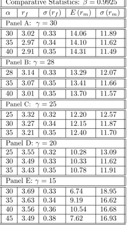
Comparative Statistics: = 0:9925 rf (rf) E(rm) (rm) Panel A: = 30 30 3:02 0:33 14:06 11:89 35 2:97 0:34 14:10 11:62 40 2:91 0:35 14:31 11:49 Panel B: = 28 28 3:14 0:33 13:29 12:07 35 3:07 0:35 13:41 11:66 40 3:01 0:35 13:70 11:57 Panel C: = 25 25 3:32 0:32 12:20 12:57 30 3:27 0:34 12:15 11:87 35 3:21 0:35 12:40 11:70 Panel D: = 20 25 3:55 0:32 10:28 13:09 30 3:49 0:33 10:33 11:62 35 3:43 0:35 10:78 11:91 Panel E: = 15 30 3:69 0:33 6:74 18:95 35 3:63 0:34 9:19 16:62 40 3:56 0:36 10:54 16:68 45 3:49 0:38 7:62 16:93
Table 4: Unconditional moments and comparative statistics. Except for the numbers in the …rst column, all other numbers are in parcentage. Columns 2-5 present the mean and the standard deviation of the risk free rate and of the
equity returns. We set = 1/1.5, and = 0.9925 in all cases.
Comparative Statistics: = 0:986 rf (rf) E(rm) (rm) Panel A: = 30 30 5:72 0:34 15:65 11:49 35 5:65 0:35 16:01 11:40 40 5:58 0:36 16:39 11:35
Table 5: Unconditional moments and comparative statistics. Except for the numbers in the …rst column, all other numbers are in parcentage. Columns 2-5 present the mean and the standard deviation of the risk free rate and of the
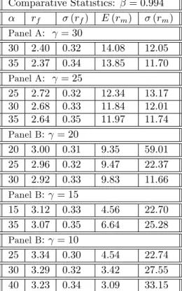
Comparative Statistics: = 0:994 rf (rf) E(rm) (rm) Panel A: = 30 30 2:40 0:32 14:08 12:05 35 2:37 0:34 13:85 11:70 Panel A: = 25 25 2:72 0:32 12:34 13:17 30 2:68 0:33 11:84 12:01 35 2:64 0:35 11:97 11:74 Panel B: = 20 20 3:00 0:31 9:35 59:01 25 2:96 0:32 9:47 22:37 30 2:92 0:33 9:83 11:66 Panel B: = 15 15 3:12 0:33 4:56 22:70 35 3:07 0:35 6:64 25:28 Panel B: = 10 25 3:34 0:30 4:54 22:74 30 3:29 0:32 3:42 27:55 40 3:23 0:34 3:09 33:15
Table 6: Unconditional moments and comparative statistics. Except for the numbers in the …rst column, all other numbers are in parcentage. Columns 2-5 present the mean and the standard deviation of the risk free rate and of the
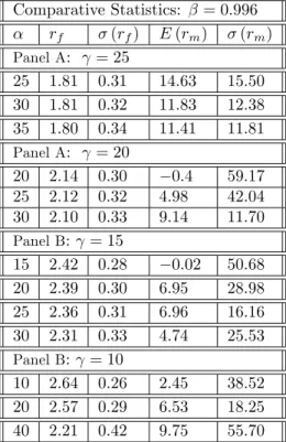
Comparative Statistics: = 0:996 rf (rf) E(rm) (rm) Panel A: = 25 25 1:81 0:31 14:63 15:50 30 1:81 0:32 11:83 12:38 35 1:80 0:34 11:41 11:81 Panel A: = 20 20 2:14 0:30 0:4 59:17 25 2:12 0:32 4:98 42:04 30 2:10 0:33 9:14 11:70 Panel B: = 15 15 2:42 0:28 0:02 50:68 20 2:39 0:30 6:95 28:98 25 2:36 0:31 6:96 16:16 30 2:31 0:33 4:74 25:53 Panel B: = 10 10 2:64 0:26 2:45 38:52 20 2:57 0:29 6:53 18:25 40 2:21 0:42 9:75 55:70
Table 7: Unconditional moments and comparative statistics. Except for the numbers in the …rst column, all other numbers are in parcentage. Columns 2-5 present the mean and the standard deviation of the risk free rate and of the
1940 1950 1960 1970 1980 1990 2000 2010 -0.04 -0.03 -0.02 -0.01 0 0.01 0.02 0.03 0.04 0.05 0.06
time serie of rate of growth of PCE, log(Ct+1/Ct)
Figure 1: Time serie of the rate of growth of Total Personal Consumption Expenditure. Data are quarterly and span the period 1947:2-2009:2. Source: BEA. 1950 1960 1970 1980 1990 2000 2010 2.8 3 3.2 3.4 3.6 3.8 4 4.2 4.4 4.6 4.8 p-d
0 0.5 1 3 3.5 4 4.5 p-d gi v en µ = hi gh P(σ = low) 0 0.5 1 3 3.5 4 4.5 p-d gi v en µ = low P(σ = low) 0 0.5 1 3 3.5 4 4.5 p-d gi v en σ = l o w P(µ = high) 0 0.5 1 3 3.5 4 4.5 P(µ = high) p-d gi v en σ = hi gh α=25 α=30 α=35
Figure 3: Price-dividend ratios ( = 25; = 1=1:5; = 4:5; = 0:9925).
0 0.5 1 0 0.05 0.1 0.15 0.2 0.25 Et (rm -rf )|σ = hi gh P(µ = high) 0 0.5 1 0 0.05 0.1 0.15 0.2 0.25 Et (rm -rf )|σ = l o w P(µ = high) α = 25 α = 30 α = 35
Figure 4: Conditional equity premium plotted as a function of the probability of high growth state. The left panel conditiones on high volatility state and the right panel on low volatility state ( = 25; = 1=1:5; = 4:5; = 0:9925).
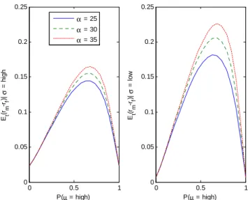
0 0.5 1 0 0.05 0.1 0.15 0.2 0.25 Et (rm -rf )|µ = hi gh P(σ = low) 0 0.5 1 0 0.05 0.1 0.15 0.2 0.25 Et (rm -rf )|µ = l o w P(σ = low) α = 25 α = 30 α = 35
Figure 5: Conditional equity premium plotted as a function of the probability of low volatility state. The left panel conditiones on high mean state and the right panel on low mean state ( = 25; = 1=1:5; = 4:5; = 0:9925).
19400 1950 1960 1970 1980 1990 2000 2010 0.1 0.2 0.3 0.4 0.5 0.6 0.7 0.8 0.9 1 P(low var) P(high mean)
Figure 6: The …gure plots the time series of estimated state probabilities. P(low variance)is the unconditional probability of being in a low consumption volatility state next period (solid line), calculated by summing the probability of being in a low volatility and high mean state and the probability of a low
volatility and low mean state. P(high mean) is calculated analogously. The
1955 1960 1965 1970 1975 1980 1985 1990 1995 2000 0 0.1 0.2 0.3 0.4 0.5 0.6 0.7 0.8 0.9 1 P(low var) P(high mean)
Figure 7: Source: Lettau et al., RFS(2008) The …gure plots the time series of
estimated state probabilities. P(low variance)is the unconditional probability of being in a low consumption volatility state next period (solid line), calculated by summing the probability of being in a low volatility and high mean state
and the probability of a low volatility and low mean state. P(high mean) is
calculated analogously. The data are quarterly and span the period 1952:1-2002:4.
1950 1960 1970 1980 1990 2000 2010 2.8 3 3.2 3.4 3.6 3.8 4 4.2 4.4 4.6 4.8 p-d data model
Figure 8: Price-dividend ratio (ambiguity neutrality).
1950 1960 1970 1980 1990 2000 2010 2.5 3 3.5 4 4.5 5 5.5 p-d data model
Figure 9: Time Series of the Price-Dividend ratio. Time series of the log price-dividend ratio from the data and implied by the model. The risk aversion
parameter and the ambiguity aversion parameters are set, respectively to =
15 and - = 20. The rate of time preferences = 0.9925 and the elasticity
of intertemporal substitution 1/ = 1.5 and leverage = 4.5. The data are
1950 1960 1970 1980 1990 2000 2010 2.8 3 3.2 3.4 3.6 3.8 4 4.2 4.4 4.6 4.8 p-d data α = 25 α = 35
Figure 10: Time series of the log price-dividend ratio from the data and implied by the model for di¤erent ambiguity aversion values. In both simluations we set
= 25; = 1=1:5; = 0:9925and = 4:5: 1950 1960 1970 1980 1990 2000 2010 2.5 3 3.5 4 4.5 5 5.5 6 p-d data model