Cognitive Ant Colony Optimization:
A New Framework in Swarm
Intelligence
Indra Chandra Joseph Riadi
Cognitive Ant Colony Optimization:
A New Framework in Swarm
Intelligence
Indra Chandra Joseph Riadi
School of Computing, Science and Engineering
College of Science and Technology
University of Salford, Manchester, UK
Tables of Contents
Tables of Contents ... i
List of Publications ... v
List of Figures ... vi
List of Tables ... viii
Acknowledgements ... ix
Declaration ... x
Abstract ... xi
Chapter 1 Introduction ... 1
1.1 Overview ... 1
1.2 Motivation ... 2
1.3 Research Objective ... 6
1.4 Research Contribution ... 7
1.5 Organization of the Thesis ... 8
Chapter 2 Survey of Ant Colony Optimization ... 9
2.1 Introduction ... 9
2.2 Foraging Behaviour of Real Ants ... 12
2.3 The Design of Artificial Ants ... 14
2.4 The Ant Colony Optimization Metaheuristic ... 15
2.6 Ant Colony Optimization Algorithms ... 20
2.6.1 Ant System ... 22
2.6.2 Elitist Ant Colony Optimization ... 26
2.6.3 Rank-based Ant System ... 27
2.6.4 MAX-MIN Ant System (MMAS) ... 28
2.6.5 Ant Colony System (ACS) ... 28
2.6.6 Hyper-Cube Framework (HFC) ... 30
2.7 The Travelling Salesman Problem (TSP) ... 31
2.8 Ant Colony Optimization Algorithm for Continuous Problems ... 33
2.9 Summary ... 34
Chapter 3 Decision-making under Risk ... 35
3.1 Introduction ... 35
3.2 Decision Making in ACO ... 37
3.3 Utility Theory ... 40
3.4 Expected Utility Theory ... 42
3.5 Prospect Theory ... 44
3.6 Summary ... 50
Chapter 4 A New Framework for Ant Colony Optimization for Discrete Optimization Problems ... 51
4.1 Introduction ... 51
4.3 Formulation of Prospect Theory in Water Distribution System (WDS)
Problems ... 56
4.4 Experimental Results ... 62
4.4.1 TSP Problems ... 62
4.4.2 Water Distribution Problems ... 68
4.5 Summary ... 74
Chapter 5 A New Framework for Ant Colony Optimization for Continuous Optimization Problems ... 77
5.1 Introduction ... 77
5.2 ACO for Continuous Domains (ACOR) ... 78
5.3 Formulation of Prospect Theory for Continuous Unconstrained Problems ... 81
5.4 Experiment Setup ... 84
5.5 Summary ... 89
Chapter 6 Analysis of the New Framework of Ant Colony Optimization Compare to Genetic Algorithm and Particles Swarm Optimization ... 91
6.1 Introduction ... 91
6.2 Comparison between ACOAs and Genetic Algorithms (GAs)... 92
6.3 Comparison between ACOAs and Particle Swarm Optimization (PSO) Algorithms ... 97
6.4 Summary ... 98
Chapter 7 Conclusions and Further Research ... 100
7.2 Future Research ... 103
Appendix A Source code in Matlab for AS-PT ... 105
Appendix B Source code in Matlab for AS-PT ... 106
Appendix C Source code in Matlab for ACS-PT ... 112
Appendix D Source code in Matlab for WDS-PT ... 119
Appendix E Sources code in Matlab for ACOR-PT ... 126
References ... 134
List of Publications
Riadi, I.C.J & Nefti-Meziani, 2011, Cognitive Ant Colony Optimization: A New Framework In Swarm Intelligence, Proceeding of the 2nd Computing, Science and Engineering Postgraduate Research Doctoral School Conference, 2011 Riadi, I.C.J & Nefti-Meziani, Ab Wahab, M.N, Ant Colony Optimization for Discrete
Domain by using Prospect Theory, is being prepared to be submitted.
Riadi, I.C.J & Nefti-Meziani, Ab Wahab, M.N, Ant Colony Optimization for Continuous Domain by using Prospect Theory, is being prepared to be submitted.
List of Figures
Figure 2.1 Leafcutter ants (Atta) bringing back cut leaves to the nest ... 10
Figure 2.2 Chains of Oecophylla longinoda ... 10
Figure 2.3 Two workers holding a larva in their mouths... 11
Figure 2.4 Double Bridge Experiments. a) The two paths are equal length. b) The lower path is twice as long as the upper path. ... 13
Figure 2.5 Basic principle of AC (Source: Blum, 2005) ... 17
Figure 2.6 ACO metaheuristic in a high-level pseudo-code ... 18
Figure 3.1 Typical utility function ... 40
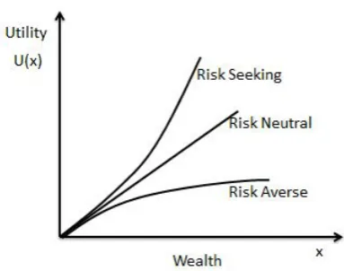
Figure 3.2 Utility functions based on wealth ... 43
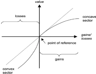
Figure 3.3 Value function ... 46
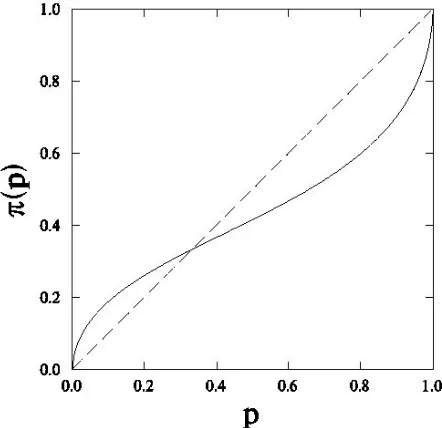
Figure 3.4 Probability weighting function ... 49
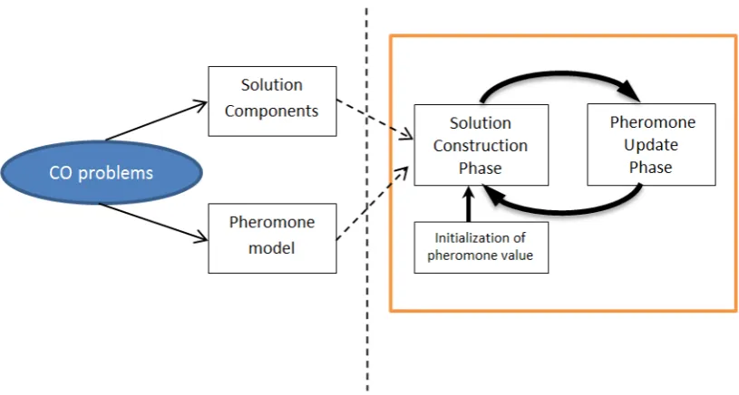
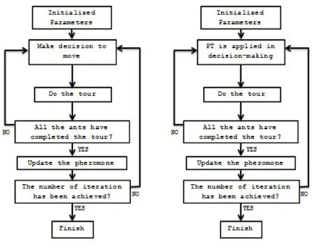
Figure 4.1 The Framework of ACO. On the left is the standard ACO and on the right is ACO-PT ... 54
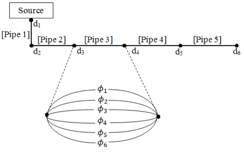
Figure 4.2 Representation of WDS Problem (Source: Maier et al., 2003) ... 57
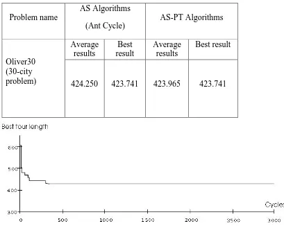
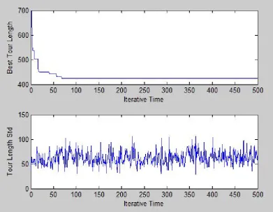
Figure 4.3 Evolution of best tour length (Oliver30). Typical run (Source: Dorigo et al., 1996) ... 63
Figure 4.4 Evolution of the standard deviation of the population’s tour lengths (Oliver30). Typical run (Source: Dorigo et al., 1996) ... 63
Figure 4.6 Typical result for ACS ... 67
Figure 4.7 Typical result for ACS-PT ... 67
Figure 4.8 New York Tunnel Problem (Source: Maier et al., 2003) ... 69
Figure 4.9 Evolving process of objective function using MMAS for NYWTP ... 70
Figure 4.10 Evolving process of objective function using MMAS+PT for NYWTP .... 71
Figure 4.11 Best fitness of each of iterations for MMAS for NYTP ... 71
Figure 4.12 Hanoi Network Problem ... 72
Figure 4.13 Typical result for MMAS for HNP ... 74
Figure 4.14 Typical result for MMAS-PT for HNP ... 74
Figure 5.1 ACOR Algorithm (Liao, et al., 2011) ... 81
Figure 5.2 The Proposed ACOR-PT Algorithm ... 85
Figure 5.3 The best result for Sphere Function, number evaluation = 840 ... 87
Figure 5.4 The best result for Ellipsoid Function, number evaluation = 300 ... 87
Figure 5.5 The best result for Brainin Function, number evaluation = 170 ... 88
Figure 5.6 The best result for Goldstein and Price Function, number evaluation = 88 .. 88
List of Tables
Acknowledgements
I would like to thank all those who have assisted me along the long route to completing this work.
Foremost, I would like to express my sincere gratitude to my supervisor Prof. Samia Nefti-Meziani for the continuous support of my PhD study and research, from initial advice and contacts in the early stages of conceptual inception and through on-going advice and encouragement to this day. Her guidance helped me in all the time of research and writing of this thesis.
I thank to all my other colleagues who have worked with me in the various aspects of this work; in particular, Ahmed Dulaimy, May Namman Bunny, Bassem Al-Alachkar, and Rosidah, to name just a few.
I would also like to thank my family for the support they provided me through my entire life and in particular, I must acknowledge my wife Ririn, and to our children; Anggraini and Setiadi for being so patient and understanding.
Declaration
Abstract
Ant Colony Optimization (ACO) algorithms which belong to metaheuristic algorithms and swarm intelligence algorithms have been the focus of much attention in the quest to solve optimization problems. These algorithms are inspired by colonies of ants foraging for food from their nest and have been considered state-of-art methods for solving both discrete and continuous optimization problems. One of the most important phases of ACO algorithms is the construction phase during which an ant builds a partial solution and develops a state transition strategy. There have been a number of studies on the state transition strategy. However, most of the research studies look at how to improve pheromone updates rather than at how the ant itself makes a decision to move from a current position to the next position.
The aim of this research is to develop a novel state transition strategy for Ant Colony Optimization algorithms that can improve the overall performance of the algorithms. The research has shown that the state transition strategy in ACO can be improved by introducing non-rational decision-making.
Chapter 1
Introduction
1.1
Overview
Ant behaviour fascinates in many ways. How can such a small creature, with the brain the size of a pinhead, be intelligent? Human beings learn to navigate in a city by exploring new knowledge or exploiting existing knowledge. Ants can also navigate in nature to find food and bring it back to their nests. However, ants cannot perform such tasks as individuals; they must be part of ant groups. Ants and other animals, such as certain birds and fish, navigate in their environment by relying on information provided by the others. This collective behaviour leads to what is called “swarm intelligence”, which was first introduced in the context of cellular robotic systems by (Beni & Wang, 1993)
circuit design, communication network design or bio-informatics problems. Some researchers have also focused on applying ACO algorithms to multi-objective problems and to dynamic or stochastic problems (Blum, 2005).
ACO algorithms have also been applied to path planning for mobile robots, which is an important task in robot navigation (Brand, Masuda, Wehner, & Yu, 2010). They enhance robotic navigation systems in both static and dynamic environments. The need of autonomous mobile robots that move faster in a dynamic, complex — even unknown — environment is of paramount importance in robotics. Without path planning, there would be a need for human operators to specify the motion for mobile robots. Autonomous path planning is essential to increase the efficiency of robot operation.
The latest overview of past and on-going research of ACO in various engineering applications can be found in Geetha & Srikanth (2012). They presented the comprehensive study of the application of ACO in diverse fields such as mobile and wireless networks, sensor networks, grid computing, P2P Computing, Pervasive computing, Data mining, Software engineering, Database systems, Multicore Processing, Artificial intelligence, Image processing, Biomedical application and also other domains relevant to Electrical Engineering fields; hence, the use of ACO algorithms is one of the most encouraging optimization techniques.
1.2
Motivation
resources, time and money. In reality, optimization problems are more complex; the parameters as well as the constraints influence the problems’ characteristics. Furthermore, optimal solutions are not always possible. We can only attain suboptimal — or even just feasible — solutions that are satisfying, robust and practically achievable in a reasonable time scale.
Uncertainty adds more complexity when searching for optimal solutions; for example, if the available materials have a certain degree of inhomogeneity that significantly affects the chosen design. Consequently, we seek not only optimal but also robust design in engineering and in industry. Moreover, most problems are nonlinear and often NP-hard, and need exponential time to find the optimum solution in terms of the problem size. The challenge is to find an effective method for search for the optimal solution, and this is not always achievable.
Many attempts have been made to improve the optimization techniques for dealing with NP-hard problems over the past few decades of computer science research. We can distinguish several high-level approaches, which are either problem-specific or metaheuristic. In the first approach, the algorithms are developed based on the problem’s characteristics derived from theoretical analysis or engineering. The second approach, the algorithms are used to find an answer to a problem when there are few or no assumptions; no clue as to what the optimal solution looks like; very little heuristic information to be followed; and where brute force search is out of the question because the space of the candidate solutions is comparatively large.
to approach a global optimum. In fact, this randomization principle is a simple and effective way to obtain algorithms with good performance for all sorts of problems. Some examples of stochastic optimization are simulated annealing, swarm intelligence algorithms and evolutionary algorithms.
Swarm intelligence algorithms derive from the social behaviour of animals that consist of a group of non-intelligent simple agents with no central control structure and no self-organization to systematise their behaviour (Engelbrecht, 2005). The local interactions between the agents and their environment lead to the emergence of global collective behaviour that is new to the individual agents. Examples of swarm intelligence algorithms are particle swarm optimization (PSO), ant colony optimization (ACO), and bee colony algorithms (BCA).
ACO algorithms are useful in problems that need to find paths to goals. Natural ants lay down pheromones directing each other to resources while exploring their environment. Artificial ants locate optimal solutions by moving through a searching space representing all possible solutions using a state transition strategy. They measure the quality of their solutions, so that in later simulation iterations more ants can locate better solutions.
colony system (ACS) algorithm, which produced better results when compared to the AS algorithm. Until now, almost all the advanced ant colony algorithms have used the pseudo-random-proportional rule.
Pseudo-random-proportional transition strategy has two main behaviours: exploitation and exploration. Exploitation behaviour is the ability of the algorithm to search through the solution space — where good solutions have previously been found — by always choosing the candidate with maximum utility. Such behaviour is rational behaviour. Exploratory behaviour is the ability of the algorithm to broadly search by randomly
choosing the candidate’s solution, which is not always that with the maximum utility. This kind of behaviour is non-rational behaviour. Higher exploitation is reflected in the rapid convergence of the algorithm to a suboptimal solution. Higher exploration results in better solutions at a higher computational cost due to the slow convergence of the method. In order to have a good result it is important to balance between these two behaviours. This is not straightforward; it needs experience and many experiments.
for human decision-making behaviour, which can be rational or non-rational depending on the way in which the problem is framed.
The ACO algorithms exhibit rational behaviour during exploitation, and they exhibit non-rational behaviour during exploration. The challenge is how to balance these two behaviours. In this thesis, we propose PT as a transition strategy in ACO algorithms. By using PT, the balance between exploration and exploitation can be adjusted by the PT model through changing the framing problem. Moreover, PT can handle the issue of how to deal with the uncertainty that has become one of the major issues in ACO optimization. By proposing to include PT in the ACO algorithms, elements of human behaviour are introduced into ACO algorithms for the first time.
1.3
Research Objective
The objective of the research is to develop a novel state transition strategy for the Ant Colony Optimization algorithms that can improve the overall performance of the algorithms. The state transition strategy in ACO algorithms is a decision-making process to select the next position during the solution construction phase, and it is very important to determine the overall performance of the algorithms.
The usage of prospect theory in ACO algorithms as a framework for a state transition strategy is investigated for the first time. This new framework will be tested in both discrete and continuous problems in order to validate the improvement of the performance that has been made. This framework is also tested in some mathematical problems and some real problems.
- To verify that the new proposed framework can be applied successfully in Ant Colony Optimization based on the prospect theory, which represents human-like decision-making under risk for both discrete and continuous optimization problems.
- To test the new framework in the travelling salesman problem (TSP), Water Distribution Systems (WDSs) and various continuous problems.
- To compare the proposed framework with the results reported in literature, based on better solutions, lower cost, a reduction in time consumption (in most cases).
1.4
Research Contribution
The research reported in this thesis contributes to the field of Ant Colony Optimization by formulating a new state transition strategy using decision-making under risk. The proposed framework provides the following unique contributions:
A novel state transition strategy model for Ant Colony Optimization based on human decision behaviour under risk is presented. The proposed model captures common human decision-making attitudes towards risk, i.e., risk aversion and risk seeking, hence improving the exploration/exploitation of Ant Colony Optimization during the iteration process.
decision-making under risk is paramount. This framework has been tested through 3 different systems to:
• Find appropriate decision variables for several optimization problems among preferred operating decision ranges.
• Find an optimal network design for a water distribution system (WDS).
1.5
Organization of the Thesis
The remainder of this thesis is organized as follows:
Chapter 2
Survey of Ant Colony
Optimization
This chapter presents a review of previous work on ACO. It contains a brief introduction, approaches to building ACO algorithms and an overview of different types of ACO algorithms.
2.1
Introduction
continuous thread of silk by squeezing larva (Figure 2.3) (Hölldobler & Wilson, 1990) (Camazine, et al., 2003).
There are many more examples that show the remarkable abilities of social insects. An insect is a complex creature that has many sensory inputs, its behaviour is controlled by many stimuli, including interactions with nest-mates, and it makes decisions on the basis of a large amount of information. Nevertheless, the complexity of an individual insect is still not sufficient to explain the complexity of what social insect colonies can achieve or how the cooperation between individuals arises.
[image:24.595.173.451.320.491.2]Figure 2.1 Leafcutter ants (Atta) bringing back cut leaves to the nest
Figure 2.3 Two workers holding a larva in their mouths
Heredity determines some of the mechanisms of cooperation, for example, anatomical differences between individuals, such as the differences between minors and majors in polymorphic species of ants, can organize the division of labour. However, many aspects of the collective activities of social insects are organized. Theories of self-organization (SO) in social insects show that complex behaviour may emerge from interactions among individuals that exhibit simple behaviour (Camazine, et al., 2003). This process is spontaneous; it is not directed or controlled by any individual. The resulting organization is wholly decentralized or distributed over all the individuals of the colony. Recent research shows that SO is indeed a major component of a wide range of collective phenomena in social insects (Serugendo, Gleizes, & Karageorgos, 2011).
There are a considerable number of researchers, mainly biologists, who study the behaviour of ants in detail. Biologists have shown experimentally that it is possible for certain ant species to find the shortest paths in foraging for food from a nest by exploiting communication based only on pheromones, an odorous chemical substance that ants can deposit and smell. This behavioural pattern has inspired computer scientists to develop algorithms for the solution of optimization problems. The first attempts in this direction appeared in the early 1990s, indicating the general validity of the approach. Ant Colony Optimization (ACO) algorithms are the most successful and widely recognized algorithmic techniques based on ant behaviours. These algorithms have been applied to numerous problems; moreover, for many problems ACO algorithms are among the current high performing algorithms.
The first ant colony optimization (ACO), called the ant system, was by Marco Dorigo and was inspired by studying the behaviour of ants in 1991 (Dorigo & Stützle, 2004). An ant colony is highly organized, in which one ant interacts with others through pheromones in perfect harmony. Optimization problems can be solved through simulating ants’ behaviours. Since the first ant system algorithm was proposed, there has been a lot of development in ACO. Since its invention, ACO has been successfully applied to a broad range of NP hard problems such as the travelling salesman problem (TSP) or the quadratic assignment problem (QAP), and is increasingly gaining interest in solving real life engineering and scientific problems. A modest survey of ACO algorithms will be presented in this chapter.
2.2
Foraging Behaviour of Real Ants
such as Lasius Niger, use a special kind of substance called pheromones to reinforce the optimum paths between food sources and their nest. To be more specific, these ants lay pheromones on the paths they take and these pheromone trails act as stimuli because the ants are attracted to follow the paths that have relatively more pheromones. Consequently, an ant that has decided to follow a path due to the pheromone trail on that path reinforces it further by laying its own pheromone too. This process can be thought of as a self-reinforcement process since the more ants follow a specific path the more likely that it becomes the path to be followed by the ants in the colony.
Deneubourg, et al. (1990) demonstrated the foraging of a colony of ants through the double-bridge experiments. In these experiments, the nest and the food sources are connected via two different paths and they examine the behaviour by varying the ratio between the lengths of the two paths as shown in Figure 2.4 (a) and Figure 2.4 (b).
Figure 2.4 Double Bridge Experiments. a) The two paths are equal length. b) The lower path is twice as long as the upper path.
result more pheromone accumulated on that path. Eventually, the whole colony converged to follow that same path. In the second experiment, the length of one path was two times as long as the other one. Initially, the ants again choose either of the two paths randomly. The ants that have chosen the shortest path arrived at the food source faster and began their return to nest earlier. Consequently, pheromone accumulated faster on the shortest path, and most of the ants converged to this path.
Deneubourg, et al. (1990) investigated further to see what would happen if a shorter path was added after the ants get convergence to one path. They found that the shorter alternative that was offered after convergence was never discovered by the colony. The majority of the ants kept following the longer branch reinforcing it more. This stagnation is caused by the fact that pheromone does not evaporate, and the real ants always follow the suboptimal optimal path even there is a shorter one. This behaviour would have to be overcome.
2.3
The Design of Artificial Ants
Real ant colonies make probabilistic movement based on the intensity of pheromone to find the shortest paths between their nest and the food source. ACO algorithms use similar agents called artificial ants. Artificial ants have the properties of the real ants. The differing characteristics of the artificial ants from the real ants were explained in (Blum, 2005):
• The real ants might not take the same path on their way to the food sources and return trip to their nest. Meanwhile, each of the artificial ants moves from the nest the food sources and follows the same path to return.
• The real ants lay pheromone whenever they move from and back to the nest. However, the artificial ants only deposit artificial pheromone on their way back to the nest.
In order to solve problems in engineering and computer science, which is the intention of ACO, some capabilities need to be added to the artificial ants which are not found in the real ants (Dorigo, Maniezzo & Colorni, 1996):
• Memory is used by artificial ants to save the path that they have taken while constructing their solutions. The amount of pheromone is determined based on the quality of their solution, and they retrace the path in their memory to deposit it. This means that the intensity of pheromone depends on the quality of the solutions. The better the solutions the more pheromones are received.
• The transition policy of artificial ants does not only depend on the pheromone trail information but also specific heuristic information. Real ants make their movement with respect to the pheromone deposits on the environment.
• Pheromone evaporation is added to encourage exploration in order to prevent the colony from trapping in a suboptimal solution whereas in real ant colonies, pheromone evaporation is too slow to be a significant part of their search mechanism.
2.4
The Ant Colony Optimization Metaheuristic
problems by using approximate methods that try to improve a candidate solution with problem-specific heuristic. Metaheuristics give a reasonably good solution in a short time, although they do not guarantee an optimal solution is ever found. Many metaheuristic implement some stochastic optimization. For example, greedy heuristic can be used to build the solution, which is constructed by taking the best action that improves the partial solution under construction. However, these heuristic methods produce a very limited variety of solutions, and they can easily get trapped in local optima. There are metaheuristic methods proposed to solve these problems; e.g. simulate annealing that guides local search heuristic to escape local optima (Dorigo & Stützle, 2004). A metaheuristic is a general framework that guides a problem specific heuristic.
In the Ant Colony Optimization, ants use heuristic information, which is available in many problems, and pheromone that they deposit along paths which guides them towards the most promising solutions. The most important feature of the ACO metaheuristic is that the ants search experience can be used by the colony as the collective experience in the form of pheromone trails on the paths, and a better solution will emerge as a result of cooperation.
• candidate solutions are constructed using probability distribution from a pheromone model;
[image:31.595.108.516.187.405.2]• the candidate solutions are used to bias the sampling by modifying the pheromone value in order to obtain high-quality solutions.
Figure 2.5 Basic principle of AC (Source: Blum, 2005)
Basically, the ACO metaheuristic is composed of 3 main phases (Dorigo and Stützle, 2004): Solution Construction Phase, Update Pheromone Phase and Daemon Actions. Each phase can be briefly described as follows:
Pheromone update phase guides the search to the region that contains high-quality solutions. In this phase, the pheromone trails are adjusted based on the latest experience of the colony. The update phase consists of decreasing and increasing the pheromone intensity on the trails. Decreasing pheromone can be achieved through pheromone evaporation. Evaporating pheromone encourages exploration and prevents stagnation. Increasing pheromone is implemented by depositing new pheromone trails on the paths used in the solutions of the ants in the previous stage. The amount of pheromone that is deposited depends on the quality of the particular solutions that each path belongs to. The paths that are used in many solutions and/or in better solutions receive more pheromone. The intensity of pheromone will be biased towards the best solution found so far. Each of ACO variants has a different pheromone update method.
Daemon actions phase is an optional phase where there is extra enhancement to the original solutions or a centralized action is implemented, which cannot be done by a single ant. For example, the use of local search methods or to lay extra pheromone to the best solution found so far.
The pseudo code of the ACO algorithm is shown in Figure 2.6.
2.5
ACO Problems
ACO algorithms are very good candidates for solving combinatorial problems since the artificial ants build the solution constructively by adding one component at a time. The ACO is also suitable for the problems where the environment may change dynamically, as ACO algorithms can be run continuously and adapted to changes in real time.
The following are characteristics that should be defined for a problem to be an ACO problem as presented in Dorigo and Stützle (2004) and Blum (2005):
• There exists a finite set of components such that𝐶= {𝑐1,𝑐2, … ,𝑐𝑛}.
• There is a set of constraints Ω defined for the problem to be solved.
• The states of the problem can be described in the form of a finite-length sequence of components such that𝑞= 〈𝑞𝑖,𝑞𝑗, … ,𝑞𝑢, …〉. Let 𝑄 denote the set of all sequences 𝑞 and 𝑄� denote the set of feasible sequence in 𝑄 satisfying the constraint Ω.
• There exists a neighbourhood structure defined between the states. 𝑞2 is a neighbour of 𝑞1 if 𝑞2 can be reached from 𝑞1 in one valid transition between the last component of 𝑞1 and the first of component of 𝑞2 and both 𝑞1 and 𝑞2 belong to 𝑄.
• There exists a set of candidate solutions 𝑆 such that 𝑆 ⊆ 𝑄 (also 𝑆 ⊆ 𝑄� if we don’t allow the unfeasible solutions to be constructed at all).
• There is a non-empty set of optimal solutions 𝑆∗ such that 𝑆∗ ⊆ 𝑄�and 𝑆∗ ⊆ 𝑆.
• There is an objective function 𝑓(𝑠) to evaluate the cost of each solutions in 𝑆.
• There may also be an objective function associated with states to be able to calculate the partial solution under construction.
correspond to the states in𝑆, a set of candidate solutions. The edges in 𝐸 correspond to valid transitions between the states in𝑆. The transition costs may be associated with the edges explicitly. Pheromone trails are associated to either the nodes or the edges, yet the latter is more common (García, Triguero, & Stützle, 2002).
In this graph, each ant in the colony searching the minimum length solution path starts from node 𝑐 in 𝐺 and stores it in its memory sequentially. The solution is gradually built by making the transition from its current state to one of the states in its neighbouring area, according to its stochastic transition policy, which is a function of the level of pheromone on the trail, problem-specific heuristic and the number of constraints defined by the problem. When the tour is complete, that is, all nodes have been visited once, the artificial ant uses its memory to evaluate its solution via the objective function and to retrace its nodes solution to create a path and deposit pheromone on it.
2.6
Ant Colony Optimization Algorithms
Some more recent ACO adaptation ideas have been proposed as a hybrid version combining ACO with other methods. Hybridization is nowadays recognized to be an essential aspect of high performing algorithms (Blum, 2005). Hybridization algorithms are more exquisite than the original one. In fact, many of the current state-of-art ACO algorithms include components and ideas originating from other optimization techniques. The earliest type of hybridization was the incorporation of local search based methods such as local search, tabu search, or iterated local search, into ACO. However, these hybridizations often reach their limits when other large-scale problem instances with a huge search space or highly constrained problems for which it is difficult to find feasible solutions are concerned. Therefore, some researchers recently started investigating the incorporation of more classical Artificial Intelligence and Operational Research methods in ACO algorithms.
2.6.1 Ant System
Construction Phase
Artificial ants construct solutions from a sequence of solution components taken from a finite set of 𝑛 available solution components𝒞= {𝑐1, … ,𝑐𝑛}. A solution construction starts with an empty partial solution 𝑆𝑝 = ∅. Then, at each construction step, the current partial solution 𝑆𝑝 is extended by adding a feasible solution component from the set𝒩(𝑆𝑝)∈ 𝒞\𝑆𝑝, which is defined by the solution construction mechanism. The process of constructing graph 𝐺𝒞 = (𝑽,𝑬) the set of solution components 𝒞 may be associated either with the set 𝑽of vertices of the graph𝐺𝒞, or with the set 𝑬of its edges.
The allowed paths 𝐺𝒞 are implicitly defined by a solution construction mechanism that defines the set 𝒩(𝑆𝑝) with respect to a partial solution𝑆𝑝. The choice of solution component from 𝒩(𝑆𝑝) is done probabilistically at each construction step. The exact rules for probabilistic choice of solution components vary across different variants of ACO.
In the example of Ant System (AS) applied to TSP the solution construction mechanism restricted the set of traversable edges to the ones that connected the ants’ current node to unvisited nodes. The choice of solution component from 𝒩(𝑆𝑝) is at each construction step performed probabilistically with respect to the pheromone model. In most ACO algorithms the respective probabilities – also called transition probabilities – are defined as follows:
𝑝(𝑐𝑖|𝑠) = [𝜏𝑖]
𝛼.[𝜂(𝑐𝑖)]𝛽
∑𝑐𝑗∈𝒩(𝑠)�𝜏𝑗�𝛼.�𝜂(𝑐𝑗)�𝛽,∀𝑐𝑖 ∈ 𝒩(𝑆
where𝜂 is an optional weighting function, that is, sometimes depending on the current sequence, assigns at each construction step a heuristic value 𝜂(𝑐𝑗) to each feasible solution component𝑐𝑗 ∈ 𝒩(𝑆𝑝). The values that are given by the weighing function are commonly called heuristic information. 𝜏𝑖 is the amount of pheromone. Furthermore, the exponents 𝛼 and 𝛽 are positive parameters whose values determine the relation between pheromone information and heuristic information. In TSP examples, we chose not to use weighting function𝜂, and we have set 𝛼 to 1. It is interesting to note that by maximizing Eq. (2-1) deterministically (i.e.𝑐 ← 𝑎𝑟𝑔𝑚𝑎𝑥{𝜂(𝑐𝑖)|𝑐𝑖 ∈ 𝒩(𝑆𝑝)}), we obtain a deterministic greedy algorithm.
Pheromone Update
Different ACO variants mainly differ in the update of the pheromone values they apply. In the following, we outline a general pheromone update rule in order to provide the basic idea. This rule consists of two parts. First, a pheromone evaporation, which uniformly decreases all the pheromone values, is performed. From a practical point of view, pheromone evaporation is needed to avoid a too rapid convergence of the algorithm towards a sub-optimal region. It implements a useful form of forgetting, favouring the exploration of new areas in the search space. Secondly, one or more solutions from the current and/or from earlier iterations are used to increase the values of pheromone trail parameters on solution components that are part of these solutions:
𝜏𝑖 ←(1− 𝜌).𝜏𝑖 + 𝜌. � 𝑤𝑠.𝐹(𝑠) �𝑠∈𝑆𝑢𝑝𝑑|𝑐𝑖∈𝑆�
2-2
so-called quality function such that𝑓(𝑠) <𝑓(𝑠′) ⟹ 𝐹(𝑠)≫ 𝐹(𝑠′),∀𝑠 ≠ 𝑠′. In other words, if the objective function value of solution s is better than the objective function value of a solution 𝑠′, the quality of solution s will be at least as high as the quality of solution𝑠′. Eq. (2-2) also allows an additional weighting of the quality function, i.e.,
𝑤𝑠 ∈ ℝ+denotes the weight of a solution𝑠.
Instantiations of this update rule are obtained by different specifications of 𝑆𝑢𝑝𝑑 and by different weight settings. In many cases, 𝑆𝑢𝑝𝑑 is composed of some of the solutions generated in the respective iteration (henceforth, denoted by 𝑆𝑖𝑡𝑒𝑟). Solution 𝑆𝑏𝑠 is often called the best-so-far solution. A well-known example is the AS-update rule, that is, the update rule of AS. The AS-update rule, which is well-known due to the fact that AS was the first ACO algorithm to be proposed in the literature, is obtained from the update rule in Eq. 2-2 by setting:
𝑆𝑢𝑝𝑑← 𝑆𝑖𝑡𝑒𝑟 and 𝑤𝑠 = 1 ∀𝑠 ∈ 𝑆𝑢𝑝𝑑 2-3
All solutions that were generated in the respective iteration are used to update the pheromone update and the weight of each of these solutions is set to 1. An example of a pheromone update rule that is used more widely in practice is the IB-update rule (where IB stands for iteration-best). The IB-update rule is given by:
𝑆𝑢𝑝𝑑 ← �𝑠𝑖𝑏 =𝑎𝑟𝑔𝑚𝑎𝑥{𝐹(𝑠)|𝑠 ∈ 𝑆𝑖𝑡𝑒𝑟}�𝑤𝑖𝑡ℎ𝑤𝑖𝑠𝑏 = 1 2-4
convergence. An even stronger bias is introduced by the BS-update rule, where BS refers to the use of the best-so-far solution𝑠𝑏𝑠. In this case, 𝑆𝑢𝑝𝑑 is set to {𝑠𝑏𝑠} and 𝑠𝑏𝑠 is weighted by 1, i.e. 𝑤𝑆𝑏𝑠 = 1. In practice, ACO algorithms that use variations of the IB-update or the BS-update rule and that additionally include mechanisms to avoid premature convergence achieve better results than algorithms that use the AS-update rule.
Eq. 2-2 shows that the pheromone update in ACO is done in 2 steps. In the first step, all pheromone trails are decreased by a constant rate𝜌, where 0 <𝜌 ≤1, due to pheromone evaporation. This evaporation in AS is implemented as Eq. 2-5 below.
𝜏𝑖𝑗 ← (1− 𝜌)𝜏𝑖𝑗 ∀(𝑖,𝑗)∈ 𝐸 2-5
In the second step, the pheromone quantities,∆𝜏𝑖𝑗, to be laid on each edge (𝑖,𝑗) are calculated according to Eq. 2-6. In this equation ∆𝜏𝑖𝑗𝑘 corresponds to the quantity of pheromone deposited by ant 𝑘 and 𝐿𝑘 stands for the cost of the solution found by ant𝑘.
∆𝜏𝑖𝑗 = � ∆𝜏𝑖𝑗𝑘 𝑚
𝑘=1
,
𝑤ℎ𝑒𝑟𝑒∆𝜏𝑖𝑗𝑘 = �
1
𝐿𝑘,𝑖𝑓𝑒𝑑𝑔𝑒(𝑖,𝑗)𝑖𝑠𝑖𝑛𝑡ℎ𝑒𝑠𝑜𝑙𝑢𝑡𝑖𝑜𝑛𝑜𝑓𝑎𝑛𝑡𝑘
0, 𝑜𝑡ℎ𝑒𝑟𝑤𝑖𝑠𝑒
𝑚𝑖𝑠𝑡ℎ𝑒𝑛𝑢𝑚𝑏𝑒𝑟𝑜𝑓𝑎𝑛𝑡𝑠
2-6
Daemon Actions
Daemon actions can be used to implement centralized control which cannot be performed by a single ant. Examples are the application of local search methods to the constructed solutions, or the collection of global information that can be used to decide whether it is useful or not to deposit additional pheromone to bias the search process from a non-local perspective. As a practical example, the daemon may decide to deposit extra pheromone on the solution components that belong to the best solution found so far.
2.6.2 Elitist Ant Colony Optimization
A first improvement on initial AS, called the elitist strategy for Ant System (EAS), was introduced in Dorigo, Maniezzo & Colorni (1996). The idea was to provide strong additional reinforcement to the edge belonging to the best tour found since the start of the algorithm; this tour is denoted as 𝑇𝑏𝑠 (best-so-far tour) in the following. Note, that this additional feedback to the best-so-far tour (which can be viewed as additional pheromone deposited by additional ant called best-so-far ant) is another example of a daemon action of the ACO metaheuristic.
Pheromone Update
𝜏𝑖𝑗 ← 𝜏𝑖𝑗 +� ∆𝜏𝑖𝑗𝑘 𝑚
𝑘=1
+𝑒∆𝜏𝑖𝑗𝑏𝑠 2-7
Where ∆𝜏𝑖𝑗𝑘 is defined as follows:
∆𝜏𝑖𝑗𝑘 = � 𝑄
𝐿𝑘 𝑖𝑓𝑗 ∈ 𝒩(𝑠)
0 𝑜𝑡ℎ𝑒𝑟𝑤𝑖𝑠𝑒 2-8
Where 𝐿𝑘 is the length of edge (𝑖,𝑗), 𝑄 is a constant parameter, and ∆𝜏𝑖𝑗𝑏𝑠 is defined as follows:
∆𝜏𝑖𝑗𝑏𝑠 = �
1
𝐶𝑏𝑠 𝑖𝑓𝑗 ∈ 𝑇𝑏𝑠
0 𝑜𝑡ℎ𝑒𝑟𝑤𝑖𝑠𝑒
𝑇𝑏𝑠is the best-so-far tour
2-9
Note that in EAS, as well as in other algorithms presented, pheromone evaporation is implemented as in Ant System.
2.6.3 Rank-based Ant System
2.6.4 MAX-MIN Ant System (MMAS)
One of the most successful ACO variants today is the MAX-MIN Ant System (MMAS) (Stützle & Hoos, 2000), which is characterized as follows. It prevents the search from becoming stagnated by imposing the quantity of pheromone trails on each edge to be in the range [𝜏𝑚𝑖𝑛,𝜏𝑚𝑎𝑥]. Depending on some convergence measure, for each of the iterations either the IB-update or BS-update rule is used for updating the pheromone values. At the start of the algorithm the IB-update rule is used more often, while during the run of the algorithm the frequency with which the BS-update rule is used is increased. MMAS algorithms use an explicit lower bound 𝜏𝑚𝑖𝑛 > 0 for the pheromone values. In addition to this lower bound, MMAS algorithms used 𝐹(𝑆𝑏𝑠)/𝜌 as an upper bound to pheromone values. The value of this bound is updated each time a new best-so-far is found by the algorithm. The best value for 𝜏𝑚𝑎𝑥 is agreed to be 1/𝜌𝐿𝑏𝑠 , where
𝐹(𝑆𝑏𝑠) = 1/𝐿𝑏𝑠, as explained in Stützle & Hoos (2000) so 𝜏𝑚𝑎𝑥 increases as shorter
paths are found by the colony. And 𝜏𝑚𝑖𝑛 is set to 𝜏𝑚𝑎𝑥/𝑎 where𝑎is a parameter. Initially, pheromone trails are set to 𝜏𝑚𝑎𝑥 on all edges; therefore ants behave in a more explorative way in the beginning. After a while, the search becomes biased towards the shortest tours found so far; however, if the colony cannot find any improved solution in a predetermined number of iterations, the pheromone trails are reinitialized.
2.6.5 Ant Colony System (ACS)
2-1. This type of solution construction is called pseudo-random proportional. So, the transition rule will be
𝑠= �arg𝑚𝑎𝑥𝑗∈𝑁𝑖𝑘{�𝜏𝑖𝑗� 𝛼
.�𝜂𝑖𝑗)�𝛽𝑖𝑓𝑞 ≤ 𝑞0 (𝑒𝑥𝑝𝑙𝑜𝑖𝑡𝑎𝑡𝑖𝑜𝑛)
𝑆, 𝑜𝑡ℎ𝑒𝑟𝑤𝑖𝑠𝑒 (𝑒𝑥𝑝𝑙𝑜𝑟𝑎𝑡𝑖𝑜𝑛) 2-10
According to this transition rule, ant 𝑘 at node 𝑖 chooses to move to node 𝑗 using the best edge in terms of the pheromone trail and heuristic value with 𝑞0 probability, therefore exploit the current knowledge of the colony. Otherwise, it selects a random node in its neighbourhood; therefore, it explores a new solution.
Second, ACS uses the BS-update rule with the additional particularity that the pheromone evaporation is only applied to values of pheromone trail parameters that belong to solution components that are in𝑆𝑏𝑠. Third, after each solution construction step, the following additional pheromone update is applied to the pheromone value 𝜏𝑖 whose corresponding solution component𝑐𝑖 was added to the solution under construction:
𝜏𝑖 ←(1− 𝜌).𝜏𝑖 + 𝜌.𝜏0 2-11
Where𝜏0 is a small positive constant such that 𝐹𝑚𝑖𝑛≥ 𝜏0 ≥ 𝑐,𝐹𝑚𝑖𝑛 ← 𝑚𝑖𝑛{𝐹(𝑠)| 𝑠 ∈
After all the ants in the colony construct their solution, only the tour corresponding to the best solution so far receives a pheromone update. As a result, the search is biased towards the vicinity of the best solutions so far. The equation 2-12 implements the global pheromone update is:
𝜏𝑖𝑗 ←(1− 𝜌)𝜏𝑖𝑗 + 𝜌∆𝜏𝑖𝑗, ∀(𝑖,𝑗) ∈ 𝑇𝑏𝑠,
where ∆𝜏𝑖𝑗 = 1/𝐿𝑏𝑠
2-12
In the equation 2-12, 𝑇𝑏𝑠 stands for the best solution so far and 𝐿𝑏𝑠stands for the cost of that solution. The parameter 𝜌 again can be thought of as the pheromone evaporation rate as in AS, but it also weighs the pheromone to be deposited in ACS. In other words, the new pheromone trails become a weighted average of the existing pheromone on the trails and the pheromone that is to be deposited (Dorigo & Stützle, 2004).
2.6.6 Hyper-Cube Framework (HFC)
algorithm applied to unconstrained problems, the average quality of the solutions produced continuously increases in asymptotically (Blum & Dorigo, 2004). The name Hyper-Cube Framework stems from the fact that with the weight setting as outlined above, the pheromone update can be interpreted as a shift in a hyper cube.
2.7
The Travelling Salesman Problem (TSP)
The TSP is considered a standard test-bed for evaluation of new algorithmic ideas for discrete optimization; indeed, good performance for TSP is considered reasonable proof of an algorithm’s usefulness. The TSP is the problem of a salesman who wants to find the shortest possible trip through a set of cities on his tour of duty, visiting each and every city exactly once.
The problem space can, essentially, be viewed as a weighted graph containing a set of nodes (cities). The objective is to find the minimal-length of a loop of the graph. To solve this problem using ACO algorithms, initially, each ant is put on a randomly chosen city. The ant has a memory which stores the partial solution that it has constructed so far (initially the memory contains only the start city). Starting from its start city, an ant iteratively moves from a city to city. When being in a city𝑖, an ant 𝑘 chooses to go to a still unvisited city 𝑗 with a probability given by
𝑝𝑖𝑗𝑘(𝑡) =�
�𝜏𝑖𝑗(𝑡)�𝛼�𝜂𝑖𝑗�𝛽
∑𝑙∈ℵ𝑖𝑘[𝜏𝑖𝑙(𝑡)]𝛼[𝜂𝑖𝑙]𝛽 𝑖𝑓𝑗 ∈ ℵ𝑖 𝑘
0 𝑜𝑡ℎ𝑒𝑟𝑤𝑖𝑠𝑒
2-13
ant𝑘, i.e. the set of cities which ant 𝑘has not yet visited. Parameters 𝛼 and 𝛽influence the algorithm behaviour. If𝛼 = 0, the selection probabilities are proportional to heuristic information and the closest cities will be more likely to be selected. In this case, AS corresponds to a classical stochastic greedy algorithm (with multiple starting points since ants are initially randomly distributed on the cities). If𝛽 = 0 , only pheromone amplification is at work. This will lead to the rapid emergence of a stagnant situation with the corresponding generation of the tours which, in general, are strongly suboptimal.
In each step of the algorithm, each ant chooses the next city based on pheromone intensity and distance which indicates a greedy approach. After completing their tours at a step t, pheromone contributions for each ant 𝑘 and edge (𝑖,𝑗) between city 𝑖 and 𝑗 are computed using
∆𝜏𝑖𝑗𝑘(𝑡) = � 𝑄
𝐿𝑘(𝑡) 𝑖𝑓𝑗 ∈ ℵ𝑖𝑘
0 𝑜𝑡ℎ𝑒𝑟𝑤𝑖𝑠𝑒 2-14
where 𝑄 is a constant and 𝐿𝑘(𝑡) is the tour length of the 𝑘-th ant. The pheromone trail is now updated using formula
𝜏𝑖𝑗(𝑡+ 1) = 𝜌𝜏𝑖𝑗(𝑡) + ∆𝜏𝑖𝑗(𝑡)
2-15 Where ∆𝜏𝑖𝑗(𝑡) is computed across all m ants
∆𝜏𝑖𝑗(𝑡) = � ∆𝜏𝑖𝑗𝑘(𝑡) 𝑚
𝑘=1
2.8
Ant Colony Optimization Algorithm for Continuous Problems
The class of optimization problems are not only discrete but there are a class of problems that require choosing values for continuous variables. These problems can be tackled by using ant algorithms for continuous function optimization with several possibilities. To apply the original ACO to continuous domain was not straightforward. One possible method is to use simplified direct simulation of the real ants’ behaviour or other method is to extend ACO metaheuristic to explore continuous spaces. This extension can be done by the suitable discretization of a search space or by probabilistic sampling.
The use of the ACO metaheuristic to solve continuous optimization problems has been reported by Liao, et al., (2011). Bilchev and Parmee (1995) proposed Continuous ACO (CACO), Monmarché, et al., (2000) suggested the API algorithm, Dréo and Siarry (2004) offered the Continuous Interacting Ant Colony (CIAC), and Socha and Dorigo (2008) recommended the extended ACO application (ACOR). The main differences of the various versions of ACO are the pheromone laying methods, the way of handling the solution construction, pheromone update and optional daemon action, and how to schedule and synchronize these components according to the characteristics of the problem being considered.
have been carried out, for example, Liao, et al. (2011) proposed Incremental Ant Colony Optimization (IACO). More detail on ACOR will be presented in Chapter 5.
2.9
Summary
Chapter 3
Decision-making under Risk
This chapter provides a general overview of decision-making under risk. We start by introducing general decision making and go on to examine decision making in ACO. This is followed by a review of decision making theory and prospect theory, which is a concept that will be used throughout this thesis.
3.1
Introduction
Decision making is an important skill for business and life. Decision making theory looks at how decisions are made and how a decision maker chooses from a set of alternatives (options) that may lead to an optimal decision. There are two goals of decision making theory: firstly, to prescribe how decisions should be made; and secondly, to describe how decisions are actually made. The first goal refers to normative decision making theory, which considers how decisions should be made in order to be rational. The second goal aims to find tools and methodologies to help people make the best decision, and relates to people’s beliefs and preferences as they are, not as they should be.
information about the probabilities of different outcomes then the decision is made under uncertainty; while if no prior knowledge is used about the probabilities the decision is made under ignorance.
Until the end of the 1970s, the best approximation to describe the decision-maker’s behaviour was the Expected Utility Theory (EUT) (Wakker, 2010). EUT has been adopted as the standard decision-making methodology used under risk conditions, but it is incapable of fully capturing actual human decision-making behaviours under uncertainty. Kahneman and Tversky (1979) proposed the prospect theory (PT) as a major breakthrough to capture this behaviour, and it was the first descriptive decision making theory that explicitly incorporated non-rational behaviour in an empirically realistic way. Later, in 1992, they introduced an improved version of PT called Cumulative Prospect Theory (CPT) (Tversky & Kahneman, 1992).
In the decision-making process, people make decisions in risky and riskless situations. The example of decision making under risk is the acceptability of a gamble that yields monetary outcomes with specific probabilities. A typical riskless decision concerns the acceptability of a transaction in which an item or a service is exchanged for money or labour, for example, to buy something. A classic decision making model under risk is a rational model which does not treat gains and losses separately, but there is much evidence that people respond differently to gains and losses.
expectation of the subjective value of monetary outcomes and not by the expectation of the objective value of these outcomes.
Kahneman, Slovic & Tversky (1982) suggest that most judgements and choices are made intuitively and the rules that direct intuition are similar to the rules of perception (visual). Intuitive judgements or choices are spontaneous, without a conscious search or computation, and without effort; however, some monitoring of the quality of mental operations and behaviour still takes place. Intuitive thinking can also be powerful and accurate. Both perception and intuitive evaluations of outcomes are reference-dependent. In standard economic analyses the utility of decision making outcomes is assumed to be determined entirely by their final stakes, and is, therefore, reference-independent (Kahneman, 2003). Preference appears to be determined by attitudes to gains and losses, defined relative to a reference point. This will cause the framing of a prospect to change the choice that the individual decision-maker makes.
This thesis proposes a novel approach for modelling human decision-makers and non-rational behaviour in ACO. This non-non-rational behaviour is based on PT (Kahneman & Tversky, 1979). This model was used to design a state transition strategy algorithm in ACO. Therefore, instead of fine-tuning the existing model the use of PT is proposed and evaluated.
3.2
Decision Making in ACO
Random-proportional rule (see Eq. 2.1) was the first idea of decision-making applied in AS. Each ant starts from a random node and makes a discrete choice to move the next edge from node 𝑖 to another node𝑗 of a partial solution. At each step, ant 𝑘 computes a set of feasible expansions, according to a probability distribution. The probability distribution is derived from a utility. This utility is computed from the pheromone intensity and the attractiveness of the edge. This pheromone can be considered as the global information and the attractiveness of the edge which is obtained from some heuristic information represents the local information. Thus, the higher the intensity of the pheromone and the value of the heuristic information are, the higher the utility is, the more profitable it is to include node 𝑗 in the partial solution. This process is usually accomplished through the use of scaling factors in the form of powers or constants boosting or shrinking an individual utility. The combination of the utility is the cornerstone to the success or failure of this technique and the combined utilities must provide an accurate deflection of the perceived strengths or weaknesses of an edge.
In an uncertain environment, the ant’s probabilistic choices during the construction of the partial solution might lead to an error and create a risk because its choices might be influenced by the ant’s attitude to that uncertainty. The common ant-selection models are based on the assumption that the ants are rational, homogenous, and have perfect knowledge. Based on these assumptions, most of the existing state-selection models use utility theory, which is based on the utility maximization assumption. However, these models do not give good results; a bias is needed to allow the ants to choose randomly using a probability distribution.
Reasons to add random choices are to make artificial ants heterogeneous in preferences, calculation errors, unobserved attributes, and insensitivity to small differences. The random component may also reflect the variations in artificial ants’ perception of the options. Utility models do not offer much insight into the way in which the ants estimate the choices. Moreover, the uncertainty presented in these models is from the view of the modeller; it provides no hypothesis as to how the ants might themselves consider uncertainty.
3.3
Utility Theory
One of the first theories of decision making under risk was based on the expected value. The expected value of an outcome is equal to its payoff times its probability. This model failed to predict the outcomes in many situations because it was apparent that the value was not always directly related to its precise monetary worth.
Daniel Bernoulli was the first to see this flaw and propose a modification to the expected value notion in 1738 in a paper entitled “Exposition of a New Theory on the Measurement of Risk (as cited in (Hansson, 1994)). In fact, Bernoulli was the first to introduce the concept of systematic bias in decision making based on a "psychophysical" mode (McDermott, 2001). By this concept, people do not always make decisions based on the expected value of the outcomes but can be influenced by such factors as the probability of the outcomes and cognitive bias. Bernoulli proposed a utility function to explain people’s behaviour in making choices. The utility function did not use a linear function of wealth, but rather a subjective one, and is concave as shown in Figure 3.1. Bernoulli assumed that people tried to maximize their utility rather than their expected value and that people are typically risk averse.
Utility Theory (UT) is an attempt to model human choice (Fishburn, 1970). The modeller knows the preferences of the decision-makers regarding the choice set, i.e. by ranking the options. The modeller must create a utility function that assigns a numerical value to each option to reflect the ranking established by decision-makers for the given choice set.
When adopting a utility function to represent the decision making process, the decisions are always deterministic, i.e. the option with the highest utility is the option chosen. According to the UT, if the utility function is correctly selected it expresses a sharp logic: “the winner takes all”.
The utility function is personal, i.e. each person has their own evaluation process – for this reason, it is called Subjective Utility Theory (SUT). Moreover, according to the UT if the attributes are kept constant, the decision does not change. The only possibility for change is if the attributes or parameters of the utility function change, but the function itself is fixed and constant. Nevertheless, the changes occur exclusively in the parameters and never in the function. Some aspects of the decision making process may remain non-captured by the model and for them a stochastic behaviour is assumed.
3.4
Expected Utility Theory
In 1944, John von Neumann and Oscar Morgenstern reinterpreted Bernoulli’s expected utility theory by proposing a formal model called expected utility theory (EUT). EUT used preferences to derive utility, in contrast to Bernoulli’s model; utility was used to define a preference, because the highest utility is more preferable. Von Neumann and Morgenstern’s axioms do not only rank the utility by an individual’s preference but also take into account the possible relationships between the individual’s preferences. As long as the relationship between an individual’s preference satisfies certain axioms such as consistency and coherence, it became possible to construct an individual utility function for that person; then the decision can be made to maximize the subjective utility.
This subjective expected utility model made no clear distinction between normative and descriptive aspects. This model assumed not only the way the decision should be made but also how people make decisions.
People seek to maximize their subjective expected utility; one person may not share the same utility curve as another, but each follows the same normative axioms in striving toward their individually defined maximum subjective expected utility.
addition, EUT predicts that the choice is invariant, that is, the way the alternatives are presented should not influence the decision makers to choose the alternatives.
The expected utility (EU) is defined as follows:
𝐸𝑈= � 𝑢(𝑥𝑖)𝑝𝑖 𝑛
𝑖=1
3-1
where 𝑢(𝑥𝑖) and 𝑝𝑖 represent the utility function of the outcome 𝑥𝑖 and probability of that outcome, respectively. The decision makers then choose the option with the highest expected utility (EU).
[image:57.595.208.400.561.712.2]In EUT, the utility is often assumed to be a function of final states or wealth. The utility function can be a concave, convex, or linear function. The concave function shows that a person is risk averse, meaning that he/she prefers the certain prospect (x) to any risky (uncertain) prospect with expected value. Thus, the preference of £50 for sure over a 50 – 50 chance of receiving £100 or nothing is an expression of risk aversion. Whereas a risk seeking person has a convex utility function meaning that he/she prefers a chance prospect over a sure outcome of greater expected utility. The one who is risk neutral has a linear utility function; he/she has no preference to the options. These behaviours are shown in Figure 3.2.
3.5
Prospect Theory
Expected utility theory has been confronted with several critiques. Some were suggestions that its underlying assumptions were unreasonable, some felt its predictions did not conform to the experimental or empirical evidence, and some of them combined the two lines of criticism. For examples, the Ellsberg paradox and the Allais paradox pointed out the deficiencies of classical expected utility theory. Numerous alternative theories have been offered, one of which is Prospect theory. Prospect theory was formulated first by Kahneman and Tversky (1979) as an alternative method of explaining choices made by individuals under conditions of risk.
Prospect theory is the most accepted description of subjected expected value decision-making by human beings. It describes the subjective human decision decision-making process, specifically in the subjective assessment of probabilities and utilities of the outcomes, and their combination in gambles (lotteries). Prospect theory suggests a nonlinear transformation of the probability scale (Kahneman & Tversky, 1979) (Tversky & Kahneman, 1992). According to the prospect theory, the value 𝑉 of a simple prospect that pays £𝑥 with probability, p and pays nothing with probability (1 – p) is given by:
𝑉(𝑥,𝑝) =𝑣(𝑥)𝑤(𝑝) 3-2
Prospect Theory divides the decision making process into two stages. The first stage is the ‘screening’ or editing stage, where probabilities and utilities are subjectively assessed, and the second stage is the ‘evaluation’ stage, where the subjective probabilities and utilities are combined. This two-staged process has three consequences. First, gains and losses are evaluated to a reference point, often assumed to be equivalent to the status quo. People are risk averse in the domain of gains and risk seeking in losses. Secondly, people tend to overweigh small probability events while underweighing medium and high probability events. Moreover, people overweigh certainty, so that they tend to treat highly probable events as certain and highly improbable events as if they were impossible. Finally, the choice of alternatives is influenced by the way the alternatives are presented (Kahneman & Tversky, 1979).
The editing stage comprises four major sequential operations, namely coding, combination, segregation, and cancelation. Coding involves the setting of a reference point by the decision-maker by which all gains and/or losses are measured. Combination consists of the aggregation of probabilities associated with identical outcomes. Segregation involves separating the risky components of the prospect from the riskless components of the prospects. Cancellation is where components shared by all prospects are discarded. Simplification is where probabilities and outcomes are simplified, such as rounding. Elimination by domination is where dominated prospect alternatives are eliminated (Kahneman & Tversky, 1979).
probabilities are overestimated and large probabilities are underestimated. Overestimated small probabilities generate optimism (high decision weight for less favourable outcomes), while underestimating large probabilities generates pessimism (low decision weight for favourable outcomes, and shows a risk averse attitude).
In the evaluation phase, the decision-maker evaluates the prospects that are attainable to him or her after the conclusion of the editing phase. The decision-maker then chooses the prospect with the highest value.
The Value Function
[image:60.595.212.410.567.720.2]In PT, the notion of “utility” is replaced by “value”. People rate value functions to gains and losses differently. Tversky & Kahneman (1979) found that people value a certain gain more than a probable gain with equal or greater expected value. Gains and losses are valued from a subjective reference point. It can be inferred from their research that the displeasure associated with losses is greater than the pleasure associated with the same amount of gains. It can be further inferred that people respond differently, depending on whether the choice is framed in terms of gains or in terms of losses. Figure 3.3 shows a graph of the value function.
There are three main characteristics of the value function in prospect theory, which are as follows:
1. It is a function of gains or losses. The reference point is used to define the gains and losses. It is a gain if an outcome is greater than the reference point and a loss if the outcome is less than the reference point.
2. It is, generally, concave for gains favouring risk aversion, and, commonly, convex for losses favouring risk seeking.
3. The function is sharply curled at the reference point, steeper for losses than for gains, that is, losses loom larger than gains and people have a tendency towards loss aversion.
One of the essential features of PT is that the overall value of a prospect is based on changes in a decision-maker’s wealth to a reference point rather than on final wealth. The new component of the PT is reference dependence. People’s value judgements are highly dependent on the reference point, that is, people are more focused on changes in their value (utility) states than the states themselves. The reference point depends on the aspect of framing. This is a bigger deviation from utility and probability weighting. This deviation is of major empirical importance. More than half of risk aversion observed has nothing to do with utility curvature or with probability weighting Instead, it is generated by loss aversion, the main empirical phenomenon regarding reference dependence (Wakker, 2010).The essence of reference dependence is not that outcomes are modelled as changes with respect some reference point (initial wealth). The reference point can change during the analysis. Deviations from a variable reference point are a major breakaway from final-wealth models.
𝑣(𝑥) = 𝑥𝛼, 𝑓𝑜𝑟𝑥 ≥0,
𝑣(𝑥) =−𝜆(−𝑥)𝛽, 𝑓𝑜𝑟𝑥 < 0,𝑤ℎ𝑒𝑟𝑒𝛼> 0,𝛽 > 0,𝜆 > 0
3-3
3-4
With loss aversion = 𝜆 > 1 𝑎𝑛𝑑𝛼 = 𝛽 (Al-Nowaihi, Bradley & Dhami, 2008), so that losses are over weighted relative to gains. The opposite, 𝜆 < 1 seeking for gains with little attention for losses. 𝜆 = 2 is interpreted as decision weight, losses are taken twice as important for decisions as gains. Overweighting can be deliberate if a decision maker thinks that more attention should be paid to losses than gains, or perceptual, with losses simply drawing more attention. The parameters of the value function, as based on the empirical study Kahnemann & Tversky (1992), were: 𝛼= 𝛽= 0.88, and 𝜆= 2.25.
Probability Weighting Function
People might be using weighting schemes to evaluate probability of the outcomes. People have tendency to over weighing very low probability events and under weighing very high probability events and this depends on how the problem is presented or framed. Also, they put a decision weight based on the probability of that outcome. This distortion of probability is captured by PT’s probability weighting function. Figure 3.4 shows the probability weighting function.
The weighting function:
π(𝑝) = 𝑝𝛾
(𝑝𝛾+(1−𝑝)𝛾)1 𝛾� 3-5