Capturing soil water and groundwater interactions with an iterative feedback coupling scheme: new HYDRUS package for MODFLOW

https://doi.org/10.5194/hess-23-637-2019 © Author(s) 2019. This work is distributed under the Creative Commons Attribution 4.0 License.

Capturing soil-water and groundwater interactions with an iterative

feedback coupling scheme: new HYDRUS package for MODFLOW

Jicai Zeng1,a, Jinzhong Yang1, Yuanyuan Zha1, and Liangsheng Shi1

1_{State Key Laboratory of Water Resources and Hydropower Engineering Science, Wuhan University, Wuhan 430072, China} a_{present address: Department of Hydrology and Atmospheric Sciences, University of Arizona, Tucson, AZ, USA}

Correspondence:Yuanyuan Zha ([email protected]) Received: 2 July 2018 – Discussion started: 16 July 2018

Revised: 16 January 2019 – Accepted: 19 January 2019 – Published: 4 February 2019

Abstract. Accurately capturing the complex soil-water and groundwater interactions is vital for describing the cou-pling between subsurface–surface–atmospheric systems in regional-scale models. The nonlinearity of Richards’ equa-tion (RE) for water flow, however, introduces numerical com-plexity to large unsaturated–saturated modeling systems. An alternative is to use quasi-3-D methods with a feedback cou-pling scheme to practically join sub-models with different properties, such as governing equations, numerical scales, and dimensionalities. In this work, to reduce the nonlinear-ity in the coupling system, two different forms of RE are switched according to the soil-water content at each numer-ical node. A rigorous multi-scale water balance analysis is carried out at the phreatic interface to link the soil-water and groundwater models at separated spatial and temporal scales. For problems with dynamic groundwater flow, the nontrivial coupling errors introduced by the saturated lateral fluxes are minimized with a moving-boundary approach. It is shown that the developed iterative feedback coupling scheme re-sults in significant error reduction and is numerically effi-cient for capturing drastic flow interactions at the water table, especially with dynamic local groundwater flow. The cou-pling scheme is developed into a new HYDRUS package for MODFLOW, which is applicable to regional-scale problems.

1 Introduction

Numerical modeling of the soil-water and groundwater in-teractions has to deal with flow components and governing equations at different scales. This adds significant complex-ity to model development and calibration. Unsaturated

soil-water and saturated groundsoil-water flows with similar proper-ties are usually integrated into a whole modeling system. Al-though physically consistent and numerically rigorous, meth-ods involving the 3-D Richards’ equation (RE; Richards, 1931) tend to be computationally expensive and numeri-cally unstable due to the large nonlinearity and the demand for dense discretization (Kumar et al., 2009; Maxwell and Miller, 2005; Panday and Huyakorn, 2004; Thoms et al., 2006; Zha et al., 2013a), especially for problems with multi-scale properties. In this work, parsimonious approaches, which appear in different governing equations and coupling schemes, are developed for modeling the soil-water and groundwater interactions at regional scales.

Simplifying the soil-water flow details into upper flux boundaries has been widely used to simulate large-scale sat-urated flow dynamics, such as the MODFLOW package and its variants (Langevin et al., 2017; Leake and Claar, 1999; McDonald and Harbaugh, 1988; Niswonger et al., 2011; Pan-day et al., 2013; Zeng et al., 2017). At the local scale, in contrast, the unsaturated flow processes are usually approx-imated with reasonable simplifications and assumptions in RE (Bailey et al., 2013; Liu et al., 2016; Paulus et al., 2013; Šim˚unek et al., 2009; van Dam et al., 2008; Yakirevich et al., 1998; Zha et al., 2013b).

The original RE, also known as themixed-formRE, takes the pressure head (h) as the driving force variable, while soil moisture content (θ) is the mass accumulation variable (Krabbenhøft, 2007). To solve the mixed-form RE, eitherh

Signif-icant improvement in mass conservation has been achieved with Celia’s modification (Celia et al., 1990). Then, efforts were made to combine the advantages in theoriginaland the

Celia-format h-form REs by switching their storage terms (Hao et al., 2005; Zadeh, 2011). However, these models still suffer from a high computational cost and low numer-ical robustness when dealing with rapidly changing atmo-spheric boundary conditions (Crevoisier et al., 2009; Zha et al., 2017). The θ-formRE, addressing the above problems, is inherently mass conservative and less nonlinear in the av-eraged nodal hydraulic diffusivity when the soil is dry (War-rick, 1991; Zha et al., 2013b). However, theθ-form RE is not applicable to saturated and heterogeneous soils (Crevoisier et al., 2009; Zha et al., 2013b). In this work, to take advantage of both forms of RE, the governing equations, rather than pri-mary variables (Diersch and Perrochet, 1999; Forsyth et al., 1995; Zha et al., 2013a), are switched at each node according to its saturation degree.

For regional problems, the vadose zone is usually concep-tualized into paralleled soil columns without lateral connec-tions. The resulting quasi-3-D coupling scheme (Kuznetsov et al., 2012; Seo et al., 2007; Xu et al., 2012; Zhu et al., 2012) significantly reduces the dimensionality and complex-ity. According to how the messages are transferred across the coupling interface, the quasi-3-D methods are catego-rized into (1) the fully coupling scheme, which simultane-ously builds the nodal hydraulic connections of sub-models at both sides and implicitly solves the assembled matrices; (2) the one-way coupling scheme, which delivers the soil-water model solutions onto the groundsoil-water model without feedback mechanism; and (3) the feedback (or two-way) cou-pling scheme, which explicitly exchanges the head and/or flux solutions in vicinity of the interface nodes.

The fully coupling scheme (Gunduz and Aral, 2005; Zhu et al., 2012) is numerically rigorous but tends to increase the computational burden under practical conditions. For exam-ple, the potentially conditional diagonal dominance causes non-convergence for the iterative solvers (Edwards, 1996). Owing to high nonlinearity in the soil-water sub-models, the assembled matrices can only be solved with unified small time steps, which adds to the computational expense. The one-way coupling scheme, as adopted by the UZF1 package for MODFLOW (Grygoruk et al., 2014; Niswonger et al., 2006) as well as the free drainage mode in SWAP package for MODFLOW (Xu et al., 2012), assumes that the water-table depth has a minor influence on flow interactions at the phreatic interface and is thus problem specific.

The feedback coupling methods, in contrast, are widely used (Kuznetsov et al., 2012; Seo et al., 2007; Shen and Phanikumar, 2010; Stoppelenburg et al., 2005; Xie et al., 2012; Xu et al., 2012) as a compromise of numerical accu-racy and computational cost. In a feedback coupling scheme, the soil-water and groundwater sub-models can be built with governing equations and numerical schemes at differ-ent scales. For flow processes with multi-scale compondiffer-ents,

such as boundary geometries, parameter heterogeneities, and hydrologic stresses, the scale-separation strategy can be im-plemented easily. Although the feedback coupling method is numerically more rigorous than a one-way coupling method, and tends to reduce the inconsistency of head and/or flux in-terfacial boundaries, some concerns arise.

The first concern is the numerical efficiency of the itera-tive and iteraitera-tive feedback coupling methods. The non-iterative approach (Twarakavi et al., 2008; Xu et al., 2012) usually leads to significant error accumulation when deal-ing with a dynamically fluctuatdeal-ing water table, especially with large time-step sizes. The iterative methods, in contrast (Kuznetsov et al., 2012; Stoppelenburg et al., 2005; Xie et al., 2012), by converging the head and/or flux solutions at the coupling interface, are numerically rigorous but computa-tionally expensive, especially when solving the coupled sub-models with a unified time-stepping scheme (Kuznetsov et al., 2012). Good balance between cost and effect is needed to maintain practical utility of the iterative feedback coupling scheme.

The second concern lies in the scale-mismatching prob-lem. For groundwater models (Harbaugh et al., 2005; Langevin et al., 2017; Lin et al., 2010; McDonald and Har-baugh, 1988), the specific yield at the phreatic surface is usu-ally represented by a simple large-scale parameter, while for soil-water models (Niswonger et al., 2006; Šim˚unek et al., 2009; Thoms et al., 2006), the small-scale phreatic water re-lease is influenced by the water-table depth and the unsat-urated soil moisture profile (Dettmann and Bechtold, 2016; Nachabe, 2002). Delivering small-scale solutions of the soil-water models onto the large-scale interfacial boundary of the groundwater model, as well as maintaining the global mass balance, usually introduces significant nonlinearity to the en-tire coupling system (Stoppelenburg et al., 2005). Condi-tioned by this, the mismatch of numerical scales in the cou-pled sub-models causes significant coupling errors and in-stability. A multi-scale water balance analysis at the phreatic surface helps to relieve such difficulties.

The third concern is the nontrivial lateral fluxes between the saturated regions controlled by the vertical soil columns, which are usually not considered in previous study (Seo et al., 2007; Xu et al., 2012). Though rigorous water bal-ance analysis is conducted to address such inadequacy (Shen and Phanikumar, 2010), the lateral fluxes solved with a 2-D groundwater model usually require additional efforts to build water budget equations in each subdivision represented by the soil columns. A moving-boundary strategy helps to avoid the saturated lateral flow in the groundwater body.

dis-parate scales. The saturated lateral fluxes between the soil columns are fully removed from the interfacial water balance equation, making it a moving-interface coupling framework. The head solution of MODFLOW 2005 (Harbaugh et al., 2005; Langevin et al., 2017) and flux solution of HYDRUS-1D (Šim˚unek et al., 2009) are relaxed to meet consistency at the phreatic surface.

In this paper, the governing equations at different scales, the multi-scale water balance analysis at the phreatic surface, and the iterative feedback coupling scheme for solving the whole system, are presented in Sect. 2. Synthetic numerical experiments are described in Sect. 3. Numerical performance of the developed model is investigated in Sect. 4. Conclu-sions are drawn in Sect. 5.

2 Methodology

To address the aforementioned first concern, governing equa-tions for subsurface flow are given at different levels of com-plexity (Sect. 2.1), numerical solutions of these equations are presented (Sect. 2.2), and nonlinearity in the soil-water sub-models is reduced by a generalized switching scheme that chooses appropriate forms of RE according to the hy-draulic conditions at each numerical node (Sect. 2.3). Then, an iterative feedback coupling scheme is developed to solve the soil-water and groundwater models at independent scales (Sect. 2.4). As for the second concern, a multi-scale wa-ter balance analysis is conducted to deal with the scale-mismatching problem at the phreatic surface (Sect. 2.5). To cope with the third concern, a moving Dirichlet boundary at the groundwater table is assigned to the soil-water sub-models (see Appendix Sect. A1); the Neumann upper bound-ary for the saturated model is provided in Sect. A2, and the relaxed iterative feedback process is presented in Sect. A3. 2.1 Governing equations

The mass conservation equation for unsaturated–saturated flow is given by

∂θ ∂t +βµs

∂h

∂t =(C+βµs) ∂h

∂t = −∇ ·q, (1)

wheret is time (T);θ (L3L−3_{) is volumetric moisture} con-tent;h(L) is the pressure head;βis 1 for the saturated region but zero for the unsaturated region;C(L−1) is the soil-water capacity (C=∂θ/∂h) for the unsaturated region but zero for saturated region;µs (L−1) is the specific elastic storage; and q(L T−1) is the vector for Darcian flux calculated by the fol-lowing:

q= −K∇H, (2)

whereK (L T−1) is the hydraulic conductivity,K=K(θ ), andH (L) is the potentiometric head, H=h+z, in which

zis the vertical location with a coordinate positive upward.

Combining Eqs. (1) and (2) results in the governing equation for groundwater flow,

µs ∂H ∂t = ∂ ∂x K∂H ∂x + ∂ ∂y K∂H ∂y + ∂ ∂z K∂H ∂z . (3) With the assumption that the horizontal unsaturated flows are negligible, the regional vadose zone is usually represented by an assembly of paralleled soil columns. The generalized 1-D RE is represented by a switchable format,

ˆ C∂ψ ∂t = ∂ ∂z ˆ K _∂ψ

∂z +1

, (4)

whereψis the primary variable. For anh-form RE,ψ=h, ˆ

C=C, andKˆ =K, while for aθ-form RE,ψ=θ,Cˆ =1, andKˆ =D; whereD (L2T−1) is the hydraulic diffusivity,

D=K/C.

2.2 Numerical approximation

The governing equation for the saturated zone (Eq. 3) is spa-tially and temporally approximated in the same form as the MODFLOW 2005 model (Harbaugh et al., 2005; Langevin et al., 2017). Celia’s modification (Celia et al., 1990; Šim˚unek et al., 2009) is applied to theh-form 1-D RE for temporal approximation. Both forms of RE are handled with a tem-porally backward finite difference discretization (Zha et al., 2013b, 2017). Each sub-model is solved by a Picard iteration scheme, which is widely used in some popular codes or soft-ware packages (van Dam et al., 2008; Šim˚unek et al., 2016). The spatial discretization of Eq. (4), as well as the water balance analysis for each node, is based on the nodal flux in elementi+1/2 (bounded by nodesiandi+1), which is

q_iψ_+1/2= − ˆ

K_ij₊+₁1_/,k₂

1zi+1/2

ψ_ij₊+₁1,k+1−ψ_ij+1,k+1

−K_ij₊+₁1_/,k₂+ε_ij₊+₁1_/,k₂, (5) where the superscriptsj andkare the levels of time and in-ner iteration, the subscript i (or i+1/2) is the number of node (or element), and1zi+1/2is the length of the element

i+1/2,1zi+1/2=(zi+1−zi). When a soil interface exists at nodei, for example, the soil moisture contents in elements

i−1/2 andi+1/2 are discontinuous at nodei, thus dissatis-fying theθ-form RE. To address this problem, the correction termεj_i++₁1_/,k₂, suggested by Zha et al. (2013b), is employed to handle the heterogeneous interface at nodesiandi+1,

εj_i++_1/21,k= ˆ K_ij₊+_1/21,k

1zi+1/2

ψ_ij₊+₁1,k−ψ_ij+1,k−

→

ψ j+1,k i+1 +

←

ψ j+1,k i

, (6)

where variables (scalar)

→ ψ

j+1,k i+1 and

← ψ

j+1,k

When ψ=h, or when ψ=θ, but no heterogeneity oc-curs, we get ψ_ij₊+₁1,k=

→ ψ

j+1,k i+1 and ψ

j+1,k

i =

← ψ

j+1,k i , so ε_ij₊+₁1_/,k₂=0. When ψ=θ, with soil interfaces at node

i or i+1,

→ ψ

j+1,k i+1 =θ

hj_i++₁1,k,p_i+1/2

and

← ψ

j+1,k

i =

θhj_i+1,k,p_i+1/2

. It is obvious that ψ_ij+1,k6=

← ψ

j+1,k i (or ψ_ij₊+₁1,k6=

→ ψ

j+1,k i+1 ), soε

j+1,k i+1/26=0.

Hereinafter,Pi+1/2represents the soil parameters in ele-menti+1/2. For example, in a van Genuchten model (van Genuchten, 1980), Pi+1/2=(θr,θs,n,m,α,ks), whereθr (L3L−3_{) andθ}

s (L3L−3) are the residual and saturated soil moisture contents;α(L−1_{),n, andmare the pore-size} distri-bution parameters,m=1−1/n; andks(L T−1) is the satu-rated hydraulic conductivity.

2.3 Switching Richards’ equation

Due to lower nonlinearity of hydraulic diffusivity (D) for dry soils (Zha et al., 2013b) and the avoidance of the mass bal-ance error by removing the soil-water capacity in the stor-age term, theθ-form RE is more robust than theh-form RE, especially when dealing with rapidly changing atmospheric boundary conditions (Zeng et al., 2018). In our work, theh -andθ-form REs are switched at each node according to its effective saturation, Se. The resulting hybrid matrix equation set is solved by the Picard iteration. The empirical effective saturation for doing switching varies with soil type and is suggested to be Secrit=0.4–0.9, the state when both theh -andθ-form REs are stable and efficient. When Se≥Secrit, the soil moisture is closer to saturation, so theh-form RE is cho-sen as the governing equation; otherwise, when it undergoes dry soil condition, theθ-form RE is preferred.

For element i+1/2, when the governing equations for nodesiandi+1 are identical, the spatial approximation of nodal flux is given by Eq. (5). When the governing equations differ at nodesiandi+1, a switched element is produced. When taking ψi=θi and ψi+1=hi+1 as an example, the nodal fluxes calculated by Eq. (5) for different forms of RE have to be carefully handled by substitutingθ_ij₊+₁1,k+1with

θ_ij₊+₁1,k, whileh_ij+1,k+1is replaced byhj_i+1,k. Whenψi =hi andψi+1=θi+1, in contrast,hj

+1,k+1

i+1 is replaced byh j+1,k i+1 , whileθ_ij+1,k+1is replaced byθ_ij+1,k. The resulting equiva-lent nodal fluxesq_ih_+1/2andq_iθ_+1/2are then weighted to ob-tain an approximation by

qi+1/2=(1−ω) qiθ+1/2+ω·qih+1/2, (7) whereωis the weighting factor, 0≤ω≤1. In our work,ω= 0.5 is applied to implicitly maintain the unknown variables of bothhj_i++₁1,k+1andθ_ij+1,k+1. Specifically, whenω=1, theh -form RE is used at nodesiandi+1; whenω=0, theθ-form RE is employed instead. A detailed study on the switching of

RE between two ends of the soil moisture condition, as well as the description of the numerical formation, can be found in Zeng et al. (2018).

Note that the equation switching method takes full advan-tage of theθ- andh-form REs, which is different from the traditional primary variable switching schemes (Diersch and Perrochet, 1999; Forsyth et al., 1995; Zha et al., 2013a). In our work, the switching-RE approach is incorporated into a new HYDRUS package.

2.4 Iterative feedback coupling scheme

The Dirichlet and Neumann boundaries are iteratively trans-ferred across the phreatic interface. The groundwater head solution serves as the head-specified lower boundary of the soil columns, while the unsaturated solution is converted into the flux-specified upper boundary of the groundwater model. Due to moderate variation of the groundwater flow, the predicted water-table solution is usually adopted in ad-vance as the Dirichlet lower boundary of the fine-scale soil-water flow models (Seo et al., 2007; Shen and Phaniku-mar, 2010; Xu et al., 2012), which in sequence then pro-vides the Neumann upper boundary for successively solving the coarse-scale groundwater flow model. Section A1 pro-vides the method for a moving Dirichlet lower boundary, while Sect. A2 presents the Neumann upper boundary for the 3-D groundwater model. In Sect. A3, the relaxed iterative feedback coupling scheme is used to solve the unsaturated– saturated sub-models at two sides of the coupling interface. 2.5 Multi-scale water balance analysis

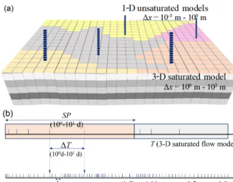
Coupling models at different scales requires consistency in their spatial and temporal scales at the interface (Downer and Ogden, 2004; Rybak et al., 2015). A space- and time-splitting strategy (see Fig. 1) is adopted to separate sub-models at dif-ferent scales. That is, the soil-water models are established by 1z=10−3–100m and1t=10−5–100 days, while for the saturated model, the grid sizes are1x=100–103m, and time-step sizes are1t=100–101days. Water balance at one side of the interface is conserved by scale matching of bound-ary conditions provided by the sub-model on the other side. For unsaturated flow, Richards’ equation requires fine dis-cretization of space and time (Miller et al., 2006; Vogel and Ippisch, 2008), while for saturated flow, coarse spatial and temporal grids produce adequate solutions at a large scale (Mehl and Hill, 2004; Zeng et al., 2017). To approximate the upper boundary flux of the groundwater flow model, a multi-scale water balance analysis is conducted within each step of the large-scale saturated flow model. At small spatial and temporal scales, e.g., within a macro-time step1T =

TJ+1−TJ and at a local area of interest (with thickness of

Bech-Figure 1. Schematic of the space- and time-splitting strategy for coupling models at two independent scales. For a groundwater model, spatial discretization is expected to be large (1x=100– 103m), while for soil-water models, it is small (1x=10−3– 100m). Multiple levels of temporal discretization are common for regional problems. For the groundwater model, the stress periods (SP) and macro-time-step sizes (1T) appear in months and days (100–101days). For soil-water models, the time-step sizes are about 10−5–100days.

told, 2016),

e

Sy=

h

w(TJ+1)−w(TJ)+θs·1zt

i

/1zt+µs·M, (8) wherew(L) is the amount of unsaturated water in the mov-ing balancmov-ing domain (see Fig. 2b), w(t )=Rzs

zt(t )θ (t, z)dz;

1zt= N

P

j=1

dzj_t =zt(TJ+1)−zt(TJ)is the total fluctuation of

the phreatic surface during1T = N

P

j=1

dtj=TJ+1−TJ, and the subscript t inzthere means the groundwater table; andθs is the saturated soil-water content. Approaching a transient state at timet, the water balance in a moving water balanc-ing domain (seez∈(zt, zs) in Fig. 2b) during a small-scale time step dt(defined in Fig. 1b) is given by

[qtop+l·dzt/2−qbot] ·dt=w(t )−w(t−dt )+θs·dzt, (9) where qtop(t ) and qbot(t ) (L T−1) are the nodal fluxes into and out of the moving balancing do-main at a fixed top boundary (zs) and a moving bot-tom boundary (zb=min(zt(t ), zt(t−dt ))), i.e., qtop=

K(h)·∂(h+z)/∂z|_z=z

s andqbot=K(h)·∂(h+z)/∂z|z=zb

(positive into the balancing domain and negative outside); dzt=zt(t )−zt(t−dt ) is the transient fluctuation of the phreatic surface during dt; andl(T−1) is the saturated lateral flux into the balancing domain at timet(see Fig. 2b). Taking

0as the lateral boundary of a sub-domain, the lateral fluxl=

R R R

x,y,z∈

h ∂ ∂x K ∂H ∂x + ∂ ∂y

K∂H_∂y

i

dxdydz/ R R R x,y,z∈

dxdydz

is supposed to be constant during1T;is the volume of the saturated domain controlled by a soil column, which is horizontally projected into5. Temporally integrating Eq. (9) from timeTJ toTJ+1produces

Rtop+εl−Rbot=w(TJ+1)−w(TJ)+θs·1zt, (10) whereRtop (L) is the cumulative water flux at zs, Rtop=

RTJ+1

TJ qtop(t )dt. Note that Rtop equals Ftop in Eq. (A3) (Sect. A2).Rbot(L) is the cumulative water flux out of the moving balancing domain,Rbot=

RTJ+1

TJ qbot(t )dt.εl (L) is the cumulative lateral input water into the moving balancing domain,

εl= 1 2l·

N

X

j=1

dtjdzj_t ε0_l=1

2l·1T ·1zt, (11) whereNis the number of time steps for the small-scale soil-water model within a macro-time step1T, andε0_lis the non-trivial saturated later flux produced by a stationary-boundary method (Seo et al., 2007; Xu et al., 2012). By takingRtopas the specific recharge atzs, the small-scale specific yieldeSyis derived from Eqs. (8) and (10) as

eSy= Rtop+εl−Rbot/1zt+µs·M. (12) Supposing that zt is linearly fluctuating in time, i.e., zt=

a·t+ b (where a and b are constants), we get the water-table change during a small-scale step (dt) by dzt=a·dt; thus,εl=o(dt2), which means that linearly refining the lo-cal time-step size (dt) in the soil-water model brings about at least quadratic approximation ofεl towards zero. Thusεl can be neglected from the small-scale mass balance analysis. In the developed model, the large-scale specific yield,Syin Eq. (A3), represents the water release in the phreatic aquifer, while the small-scaleeSyin Eq. (12) denotes the dynamically changing water yield caused by the fluctuation of the wa-ter table. The upper boundary fluxFtopin the phreatic flow equation (Eq. A3) is therefore corrected to

Ftop=

Rtop+(Sy−eSy)1zt

/1T . (13)

Differing from previous studies (Seo et al., 2007; Shen and Phanikumar, 2010; Xu et al., 2012), a scale-separation strat-egy is employed in Eq. (13). The specific yields at two differ-ent scales are explicitly linked inFtop. The large-scale prop-erties in the groundwater model (MODFLOW) are thus fully maintained.

3 Numerical experiments

Figure 2.The Dirichlet–Neumann coupling of the soil-water and groundwater flow models at different scales. (a) Linear or step-wise prediction of Dirichlet lower boundary for the soil-water flow model. (b) Water balance analysis based on a balancing domain with moving lower boundary. Blue dashed line is the linearly extrap-olated groundwater table as an alternative for prediction of Dirichlet lower boundary.J(orj),T(ort), and1T(or dt) are the time level, time, and time-step size at coarse (or fine) scale. At any of the tran-sient states (t), the balancing domain is bounded by a user-specified top elevation (zs) and the moving phreatic surface (zt). At a tran-sient timet(orTJ), the total mass volume in the moving balancing domain is indicated byw(t )(orw(TJ)). The saturated lateral flux of the moving domain is indicated byl(t ), while the unsaturated lat-eral flux is neglected as the assumption of quasi-3-D models. The water flux into and out of the balancing domain is indicated byqtop andq_bot.

solutions are obtained from the fully 3-D variably saturated flow (VSF; Thoms et al., 2006) model. At the regional scale, a synthetic case study suggested by Twarakavi et al. (2008) is reproduced. The codes are run on a personal computer with a 16 GB RAM and 3.6 GHz Intel Core (i3-4160). A maximal number of feedback iterations is set at 20. Soil parameters for the van Genuchten model (van Genuchten, 1980) are given in Table 1. The root-mean-square error (RMSE) of the solution

ψat timetis given by

RMSE(ψ, t )=

(

1

N

N

X

i=1

ψ_iref(x, t )−ψi(x, t )

2 )1/2

, (14)

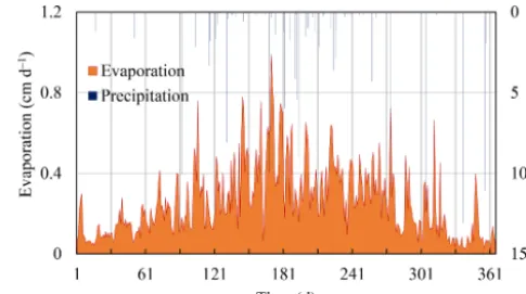
Figure 3.Rapidly changing atmospheric upper boundary conditions for scenario 2, case 1.

whereψis the numerical solution of either the pressure head or water content,ψref is the corresponding reference solu-tion, and subscripti is the number of nodes,i=1, 2, . . . ,

N.

3.1 Case 1: rapidly changing atmospheric boundaries The 1-D case is used to investigate the benefit brought by switching Richards’ equation in the unsaturated zone. A soil column is initialized with a hydrostatic water-table depth of 800 cm. That is,h(t=0, z)=200−zcm, withz=0 at the bottom and z=1000 cm on the top. The lower boundary is set to non-flux to avoid the extra computational burden caused by variation of the groundwater model. Two scenar-ios from literature are reproduced with rapidly changing up-per boundaries, as well as extreme flow interactions between the unsaturated and saturated zones.

Miller et al.’s problem (Miller et al., 1998) is reproduced in scenario 1. A dry sandy soil column (see soil no. 1 in Ta-ble 1) experiences a large constant flux infiltration at the soil surface ofqtop=30 cm days−1, which ceases att=4 days.

In scenario 2, Hills et al.’s problem (Hills et al., 1989) is considered. The soils no. 2 and no. 3 from Table 1 are alterna-tively layered with a thickness of 20 cm within the first 80 cm of depth. Below 80 cm (z=0–920 cm) is soil no. 2, with a non-flux bottom boundary. The atmospheric upper bound-ary conditions, rainfall and evaporation, change rapidly with time (see Fig. 3), over 365 days.

The coupled unsaturated model is discretized into a fine grid with1z=1 cm, while the saturated model is discretized into two layers with thickness of 500 cm. The impact of dif-ferent numbers of feedback iteration, closure criteria, and different forms of the 1-D Richards’ equation are investi-gated. Solutions obtained from the HYDRUS-1D model with

Table 1.Soil parameters used in the test cases.

no. soil θr θs α n ks

(cm3cm−3) (cm3cm−3) (cm−1) (cm days−1)

1 Sand 0.093 0.301 0.0547 4.264 504

2 Berino loamy fine sand 0.029 0.366 0.028 2.239 541 3 Glendale clay loam 0.106 0.469 0.010 1.395 13.1

4 Loam 0.078 0.430 0.036 1.560 24.96

5 Sandy loam 0.065 0.410 0.075 1.890 106.1

Figure 4.Schematic of the cross section for test case 2. Two pump-ing wells with screens ofz=0–200 cm are located atx=2500 and 5000 cm. The pumping rates per unit width at well no. 1 and no. 2 are 2×104and 1×104cm2days−1, respectively.

3.2 Case 2: dynamic groundwater flow

A 2-D case is analyzed with sharp groundwater flow (see Fig. 4). To minimize the unsaturated lateral flow, the soil surface is set with a non-flux boundary. The bottom and lateral boundaries are also non-flux. Two pumping stresses are applied to the cross-sectional field withx×z= 5000 cm×1000 cm. Well no. 1 is located at x=2500 cm, with a pumping screen at z=0–200 cm, while well no. 2 is atx=5000 cm, with a pumping screen ofz=0–200 cm. Pumping rates for wells no. 1 and no. 2 respectively are 2×104and 1×104cm2 days−1per unit width. The initial hydrostatic head of the cross section is h0(x, z)=700 cm. Soil no. 4 in Table 1 fills the entire cross section. The to-tal simulation lasts 50 days. For the coupled saturated sub-model, as well as the reference model (VSF Thoms et al., 2006), the cross section is discretized horizontally into uni-form segments with a width 1x=50 cm, while vertically (bottom up) refined into segments with thicknesses 1z= 200 cm(×1), 100 cm(×2), 50 cm(×2), 25 cm(×2), 12.5 cm(×4), and 5 cm(×200), where the subscripts hereinafter (×N) are the numbers of discretized segments. The 1-D soil-water models are discretized with a segmental thickness of1z= 1 cm. The fully 2-D unsaturated–saturated solutions from the VSF model are taken as the truth.

Table 2.The precipitation, evaporation, and pumping rates in 12 stress periods.

Stress period Precipitation Evaporation Pumping rate (mm days)−1 (mm days)−1 (m3days−1)

1 0.21 1.32 4078

2 1.69 1.32 4078

3 2.11 1.32 2039

4 4.21 1.32 2039

5 1.05 1.32 6116

6 2.11 1.32 0

7 0.63 1.32 4078

8 1.05 1.32 0

9 0.63 1.32 2039

10 0.42 1.32 0

11 0.21 1.32 6116

12 0.21 1.32 0

3.3 Case 3: pumping and irrigation

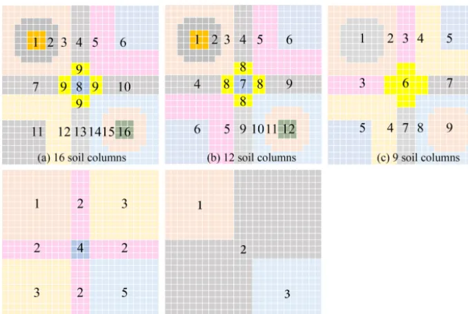
Figure 5.Different number of subzones partitioned for the quasi-3-D simulations in case 3. The vadose zone is partitioned into 16, 12, 9, 5, and 3 subzones.

3.4 Case 4: synthetic regional case study

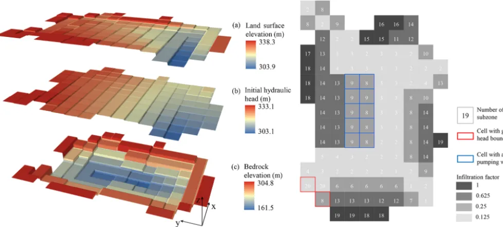
A hypothetical test case from literature (Niswonger et al., 2006; Prudic et al., 2004; Twarakavi et al., 2008) for a large-scale simulation is reproduced here. The overall alluvial basin is divided into uniform grids with1x=1y=1524 m. The coupled saturated model is conceptualized into a single layer. The initial head, as well as the elevations of land sur-face and bedrock, are presented in Fig. 6a, b, and c. The pre-cipitation, evaporation, and pumping rates for 12 stress peri-ods, each lasting 1/12 of 365 days, are given in Table 2. The infiltration factors (see Fig. 6d) are used to approximate the spatial variability of precipitation. The initial head in the va-dose zone is set with hydrostatic status. Twenty soil columns, coinciding with the subzones in Fig. 6d, are discretized sep-arately with a range of gradually refined segments with a thickness (1z) from 30.48 to 0.3048 cm (bottom up). A com-parative analysis is conducted with the solutions obtained from the original HYDRUS package for MODFLOW (taken as HPM for short; Seo et al., 2007).

4 Results and discussion

4.1 Reducing the complexity of a feedback coupling system

The numerical difficulty in a coupled unsaturated–saturated flow system originates from the nonlinearity of the soil-water models, heterogeneity of the parameters, and the variabil-ity of the hydrologic stresses (Krabbenhøft, 2007; Zha et al., 2017). In our work, the overall complexity of an iteratively

coupled quasi-3-D model could be lowered by (1) taking full advantage of theh- andθ-form REs to reduce the nonlinear-ity in the soil-water models and (2) smoothing the variabilnonlinear-ity in the exchanged interfacial messages.

Figure 6.Input of the synthetic regional problem including(a)land surface elevation,(b)initial head,(c)bedrock elevation of the aquifer, and(d)the subzones and boundaries.

with the switching scheme, while it was solved 10 925 times for the HYDRUS-1D code. The switched governing equa-tions contribute toward cutting the computational cost by half for problems with rapidly changing upper boundary condi-tions. Here, the threshold for choosing an appropriate form of RE was non-sensitive to the numerical efficiency. A wide range of Secrit[0.3, 0.9] was suggested according to sub-stantial trial-and-error tests.

Reducing the complexity of a coupling system can also be attained by smoothing the exchanged information in space and time. As suggested by Stoppelenburg et al. (2005), a time-varying specific yield calculated by the small-scale soil-water models,eSyin Eq. (12), introduced significant variabil-ity to the large-scale groundwater model, thus caused extra iterations. A large-scale Sy reduced the nonlinearity of the storage term in the groundwater equation. In case 1, using an

Sy of 0.1–0.2 in the groundwater model produced best nu-merical stability for the sandy soil with dramatically upris-ing water table. With a large-scaleSy, the nonlinearity intro-duced by the small-scale soil-water models could be quickly smoothed, as shown in Eq. (12).

4.2 Multi-scale water balance analysis

The traditional non-iterative feedback coupling methods can-not maintain sound mass balance near the phreatic surface, especially for problems with drastic flow interactions.

One reason is that, to launch a new step of a sub-model at either side of the phreatic interface, the non-iterative feedback methods usually employed a predicted interfacial boundary without correction, which inevitably introduced coupling errors. In traditional non-iterative methods (Seo et

al., 2007; Xu et al., 2012), such shortcomings could be al-leviated by refining the macro-time-step size (1T). How-ever, the Dirichlet head predicted for the soil columns with a stepwise extension method (see Fig. 2a) was easy to im-plement but tended to suffer from significant coupling error. In this work, we proposed a linear extrapolation method for the lower boundary head prediction for the soil-water mod-els (see Eq. A2). Here, we used niter to indicate the max-imal number of feedback iteration. Compared with a tra-ditional stepwise method, the solution obtained by a linear method, either iteratively (with niter=3) or non-iteratively (niter=0), was easier for approaching the truth (see Fig. 9). Even with refined macro-time-step sizes (1T from 0.2 to 0.005 days), the stepwise method made a thorough effort to minimize the coupling errors. Notably, three feedback iter-ations (niter=3) were sufficient for reducing the coupling error significantly. Such a one-dimensional case with con-stant upper boundary flux, avoiding interference from lat-eral fluxes, illustrated the importance of a temporal scale-matching analysis for coupling the soil-water and groundwa-ter models.

Figure 7. The time-step sizes through the simulation of (a)sudden infiltration into a dry sandy soil column and(b)rapidly changing atmospheric upper boundary conditions with a layered soil column.

Figure 8. Comparison of soil moisture content atz=0, 50, and 200 cm for the layered soil column with rapidly changing upper boundary conditions (scenario 2, case 1). Taking the HYDRUS-1D solution as the truth, RMSEs of solution of the developed model are provided at different soil depths.

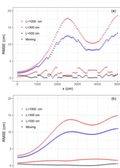
vertically distributed fine-scale source and sink terms for the soil columns, an extra downscaling approach is needed to en-sure their accuracy. Here we carried out a multi-scale water balance analysis above the phreatic surface. The fine-scale saturated lateral flows were thus excluded from Eq. (10). The benefits of the moving-boundary approach can be seen in case 2, which produces significant saturated lateral flux. We carried out a comparative analysis against the traditional stationary-boundary methods (Seo et al., 2007; Xu et al., 2012). The 2-D solution of VSF was taken as the truth. Fig-ure 10 presents the effectiveness of the moving-boundary method. Five stationary soil columns with three different lengths (L=1000, 500, and 300 cm) were compared with an adaptively moving soil column within the iterative feedback coupling scheme. The cross-sectional RMSE of the phreatic surface and the head at the bottom layer (z=0) are presented in Fig. 10a and b. The soil columns with bottom nodes fixed deeply into the aquifer, instead of moving with the phreatic surface, introduced large coupling errors. This was caused

by the nontrivial saturated lateral fluxes between the ad-jacent soil columns. With a traditional stationary-boundary method, such problems can be alleviated by avoiding large saturated lateral fluxes between the soil columns. However, for some spatiotemporally varying local events in a regional aquifer (e.g., pumping or flooding irrigation), such problems increased the burden for subzone partitioning. A moving-boundary method, instead, was numerically more efficient in minimizing the size of the matrix equation and reducing the coupling errors.

4.3 Regulating the feedback iterations

In coupling two complicated modeling systems, a common agreement has been reached that; feedback coupling, either iteratively (Markstrom et al., 2008; Mehl and Hill, 2013; Stoppelenburg et al., 2005; Xie et al., 2012) or non-iteratively (Seo et al., 2007; Shen and Phanikumar, 2010; Xu et al., 2012), is numerically more rigorous than the one-way cou-pling scheme. The main difference between the above two methods lies in the ability to conserve mass within a single step for back-and-forth information exchange. In an iterative method, the head and/or flux boundaries are iteratively ex-changed. There is a cost–benefit tradeoff for obtaining higher numerical efficiency.

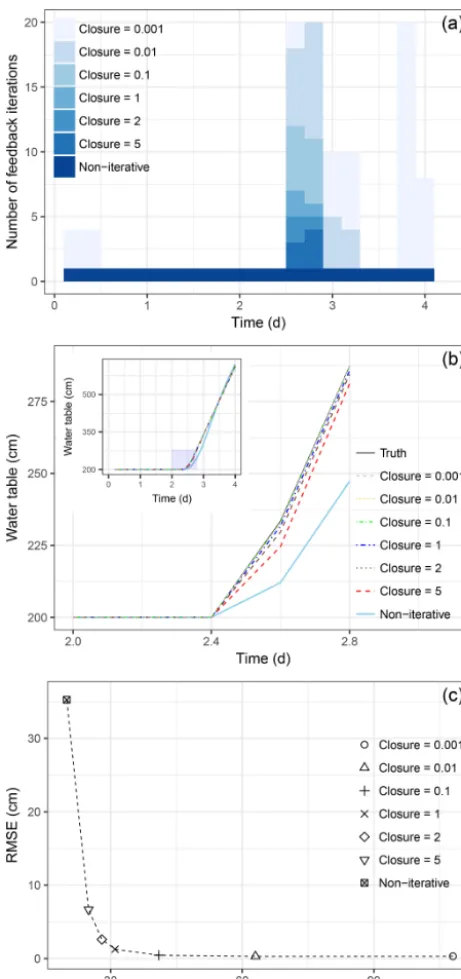
During the late stages of the recharge in scenario 1 of case 1, the groundwater table rises quickly, which increases the burden on the coupling scheme. In our work, feedback iter-ation was conducted to eliminate the coupling error within the back-and-forth boundary exchange. To investigate how the feedback iteration influences the numerical accuracy as well as computational cost, solutions were compared with different closure criteria, instead of different maximal num-bers of feedback iterations. For this purpose, scenario 1 in case 1 is tested with a range of closure criteria indicated by closure=0.001, 0.01, 0.1, 1, 5, and 20. Specifically, clo-sure=20 (i.e.,εH=20 cm) is too large to regulate any feed-back iteration and is thus replaced by “non-iterative”. The

feed-Figure 9.Water table changing with time for different macro-time-step sizes (1T=0.005, 0.05, 0.1, and 0.2 days), in scenario 1, case 1. The HYDRUS-1D solution is taken as the truth. Compared with the stepwise extended method (Seo et al., 2007), the coupling error is significantly reduced by a linear prediction.

Figure 10.Comparison of RMSE of(a)the phreatic surface and

(b)the head solution (atz=0) between the moving-boundary and the stationary-boundary methods. Three different lengths of the sta-tionary soil columns,L=1000, 500, and 300 cm, are considered.

back iteration, is usually related to the phreatic Darcian flux. To avoid its impact on the discussion below, we assume that

εF= +∞, which means no regulation from the flux bound-ary exchange. Due to less dynamic in the groundwater sub-model, the empirical relaxation factors were both set by 1.0

to have a straightforward update of the interfacial boundaries, i.e.,ztandFtop.

When the wetting front approached the phreatic surface (at

t=2.4 days), the number of feedback iterations increased dramatically (see Fig. 11a). This was caused by the inten-sive rise of the water table within each macro-time step1T. The head and/or flux interfacial boundaries were thus not easy to approximate the truth. With several attempts to ex-change the head and/or flux boundaries, the head solution was effectively drawn towards the truth, (see Fig. 11b). With closure<2, i.e.,εH<2 cm, the coupling errors were signifi-cantly reduced (see Fig. 11c). The cost–benefit curve, which was quantified by the number of feedback iteration and the RMSE, was indicative of problems at larger scales and higher dimensionalities.

4.4 Parsimonious decision-making

The feedback coupling schemes, either iteratively or non-iteratively, increase the degree of freedom of the users to manage the sub-models with different governing equations, numerical algorithms, and the heterogeneities in parameters and variabilities in hydrologic stresses. For practical pur-poses, a significant concern is how to efficiently handle the complicated and scale-disparate systems.

Figure 11. (a)The number of feedback iterations and(b)phreatic surface solutions changing with different closure criteria. In the leg-end, “closure=0.001” means thatεH=0.001 cm is used to regu-late the feedback iteration. The HYDRUS-1D solution is taken as truth. Tested in scenario 1, case 1.

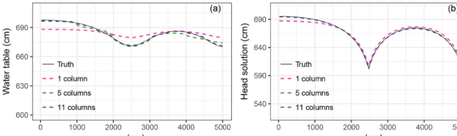
In case 3, a simple pumped and irrigated region was sim-ulated with different numbers of soil columns. A range of tests with total numbers of 16, 12, 9, 5, and 3 soil columns were carried out to obtain a cost–benefit curve, shown in Fig. 13c. When partitioning the vadose zone into more than 12 soil columns, there was a slight reduction in solution er-rors (RMSE) and a significant increase in the computational

cost caused by solving more 1-D soil-water models. Al-though parallelled computation could further reduce the nu-merical cost, representing the vadose zone with three sequen-tially calculated soil-water models achieved acceptable accu-racy, as presented in Fig. 13a and b. The computational cost for obtaining the fully 3-D solution with VSF was 15.561 s, which was more than 11 times larger than an iterative feed-back coupling method with soil-water models sequentially solved. Problems in more complicated real-world situations can thus be simplified to achieve higher numerical efficiency. 4.5 Regional application

Prudic et al.’s problem was originally designed to validate a streamflow routing package (Prudic et al., 2004). Stressed by soil surface infiltration, pumping wells, and the general head boundary, the synthetic case was used to evaluate sev-eral unsaturated flow packages for MODFLOW (Twarakavi et al., 2008). Based on their studies, in case 4, we compared the developed iterative feedback coupling method with HPM. The hydraulic conductivity, as well as its heterogeneity, was forced to be consistent within the saturated and unsaturated zones, which is different from the case in Twarakavi et al. (2008). Figure 14a gives the contours for the final phreatic head solutions, indicating a good match of the phreatic sur-face with the HYDRUS package. Figure 14b–e present the absolute head difference of the method developed here and the HYDRUS package at the end of stress periods 3, 6, 9, and 12. The dark color blocks indicated the largest differ-ence in the head solution. According to Fig. 6d, the satu-rated grid cells controlled by the soil columns of no. 3, no. 9, no. 10, no. 15, and no. 19 were suffering from the largest deviation, although with the same horizontal partitioning of the unsaturated zone. The strict iteratively two-way coupling contributes to such an accuracy improvement.

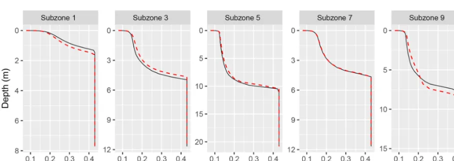
For unsaturated–saturated flow situations, the vadose zone flow is important. Figure 15 presents the water content pro-files at subzones 1, 3, 5, 7, and 9 as examples. The solution obtained from the developed model matched well with the original HPM solution. For practical purposes, the manually controlled stress periods for the unsaturated sub-models are no longer constrained. In our method, the soil-water models run at disparate numerical scales, which makes it possible to handle daily or hourly observed information rather than a stress period lasting 2 or more days in traditional coupled models.

5 Summary and conclusions

Figure 12.Comparison of(a)water table and(b)head solution (atz=0) that are changing by the number of soil columns. Solutions obtained with a moving-boundary method in case 2.

Figure 13. (a)Comparison of contours of the phreatic surface solution obtained with the fully 3-D and quasi-3-D methods.(b)Comparison of the phreatic surface at A–A’ cross section;(c)computational cost and RMSE changing by the number of total soil columns.

problem. Such a simplification brings about computational cost saving and flexibility for better manipulation of the sub-models. However, the nonlinearity in the soil-water reten-tion curve, as well as the variability in realistic boundary stresses of the vadose and saturated zones, usually results in the scale-mismatching problems when attempting numer-ical coupling. In this work, the soil-water and groundwater models were coupled with an iterative feedback (two-way) coupling scheme. Three concerns about the multi-scale water balance at the phreatic interface are addressed using a range of numerical cases in multiple dimensionalities. We conclude with the following:

1. A new HYDRUS package for MODFLOW was devel-oped by switching theθandhforms of Richards’ equa-tion (RE) at each numerical node. The switching RE cir-cumvents the disadvantages of theh- andθ-form REs to achieve higher numerical stability and computational efficiency. The one-dimensional switching RE was

em-ployed to simulate the rapid infiltration into a dry sandy soil, and the swiftly altering atmospheric upper bound-aries in a layered soil column. Compared with theh -form RE, the switching RE used a 105times larger min-imal time-step size (1tmin) and conserved mass better. Lowering the nonlinearity of soil-water models with this switching scheme was promising for coupling complex flow modeling systems at the regional scale.

soil-Figure 14. (a)Comparison of elevation of the water table calculated by the HYDRUS package for MODFLOW (Seo et al., 2007) and the developed method (t=365 days).(b)The absolute head difference of the phreatic head solution by the method developed here and HYDRUS package at the end of stress periods 3, 6, 9, and 12 (case 4).

Figure 15.Comparison of water content profiles obtained from the HYDRUS package for MODFLOW (Seo et al., 2007) and the developed iterative feedback coupling method. Subzones 1, 3, 5, 7, and 9 are shown as an example. (t=365 days in case 4).

water and groundwater interactions, the coupling errors were significantly reduced by using an iterative feed-back coupling scheme. The multi-scale water balance analysis mathematically maintained numerical stabili-ties in the sub-models at disparate scales.

3. When a moving phreatic boundary was assigned to the soil columns during the phreatic water balance analy-sis, it avoided the coupling errors originating from the saturated lateral fluxes. In practical applications for re-gional problems, the fluxes into and out of the saturated parts of the soil columns differed, which added to the

complexity and phreatic water balance error of the cou-pling scheme. With a moving Dirichlet lower boundary, the saturated regions of the soil-water models were re-moved. The coupling error was significantly reduced for problems with major groundwater flow. Extra cost sav-ing was achieved by minimizsav-ing the matrix sizes of the soil-water models.

will be coupled in an object-oriented modeling system. The RS- and GIS-based data class can then be used to handle more complicated large-scale problems.

Appendix A

A1 The moving Dirichlet lower boundary

The bottom node of a soil column is adaptively located at the phreatic surface, which makes it an area-averaged moving Dirichlet boundary:

zt(T )=

Z

s∈5

H (T )ds/

Z

s∈5

ds, (A1)

wherezt(T )(L) is the elevation of the water table;5is the control domain of a soil column;H (T )(L) is potentiometric head solution, as well as the elevation of the phreatic surface, which is obtained by solving the groundwater model; ands

is the horizontal area.

To simulate the multi-scale flow process within a macro-time step1TJ+1=TJ+1−TJ, the lower boundary head of a soil column is temporally predicted either by stepwise exten-sion ofzt(TJ)(Seo et al., 2007; Shen and Phanikumar, 2010; Xu et al., 2012) or by linear extrapolation fromzt(TJ+1)and

zt(TJ). In Fig. 2a, the stepwise extension method (z0t(TJ)) potentially causes large deviation from the truth. In our study, the linear extrapolation is resorted to for reducing the cou-pling errors and accelerating the convergence of the feed-back iteration. The small-scale lower boundary head at time

t (TJ< t≤TJ+1) is given by

zt(t )=

(t−TJ−1)·zt(TJ)−(t−TJ)·zt(TJ−1)

TJ_−TJ−1 . (A2)

A2 The Neumann upper boundary

The moving Dirichlet boundary introduces the need for water balance of a moving balancing domain above the water table (see Fig. 2b), which is bounded by a specific elevation above the phreatic surface, zs (L), and the dynamically changing phreatic surface,zt(t )(L).

Assuming that the activated top layer in a three-dimensional groundwater model is conceptualized into a phreatic aquifer, the governing equation for this layer is given by

Sy

∂H

∂t = ∂

∂x

KM∂H ∂x

+ ∂ ∂y

KM∂H ∂y

+Ftop−Fbase, (A3) where M (L) is the thickness of the phreatic layer, which is numerically defined as the layer below the vadose zone,

M=zs−z0;z0 is the bottom elevation of the top phreatic layer, z0zs; Ftop (L T−1) is the groundwater recharge into the activated top layer of the phreatic aquifer, Ftop=

(K·∂H /∂z)_z=zs; andFbaseis the leakage into an underlying

numerical layer, Fbase=(K·∂H /∂z)z=z0 (positive

down-ward, likeFtop). The long-term regional-scale parameter in-dicating the water yield caused by the fluctuation of the water table (Nachabe, 2002),Sy, (–), is calculated by

Sy=Vw/(A·1H ), (A4)

Figure A1.Flowchart of the relaxed iterative feedback coupling scheme. The relaxation is conducted at the interfacial Dirichlet– Neumann boundaries during the feedback iterations (except for the timeTJ).

whereVw(L3) is the amount of water release caused by fluc-tuation of the phreatic surface (1H (L)), andA(L2) is the area of interest.

A3 The relaxed iterative feedback coupling

The relaxed feedback iteration method (Funaro et al., 1988; Mehl and Hill, 2013) is used to improve the convergence of head and/or flux at the phreatic surface (see Fig. A1). The Dirichlet lower boundary head for the soil columns, zt, as well as the Neumann upper boundary flux for the phreatic surface,Ftop, are updated within each iterative step (niter):

zupdated_t =λh·znewt +(1−λh)·zoldt , (A5)

F_topupdated=λf ·Ftopnew+(1−λf)·Ftopold, (A6) where superscripts old (or new) indicate the previous (or newly calculated) head and/or flux boundaries at the coupling interface, andλhandλf are the empirical relaxation factors for head and/or flux boundaries respectively. Their values are suggested to be within 0< λ≤1. The iteration ends when agreements are reached at

z

updated t −zoldt

≤εHand F

updated top −Ftopold

≤εF, (A7)

Author contributions. JZ, YZ, and JY developed the new package for soil-water movement based on a switching Richards’ equation; JZ and YZ developed the coupling methods for efficiently joining the sub-models. JZ, YZ, JY, and LS made non-negligible efforts in preparing the paper.

Competing interests. The authors declare that they have no conflict of interest.

Acknowledgements. This work was funded by the Chinese Na-tional Natural Science Foundation (no. 51479143 and 51609173). The authors would thank Ian White and Wenzhi Zeng for their laborious revisions and helpful suggestions for the paper as well as the editorial team for the HESS Journal.

Edited by: Bob Su

Reviewed by: two anonymous referees

References

Bailey, R. T., Morway, E. D., Niswonger, R. G., and Gates, T. K.: Modeling variably saturated multispecies reactive groundwater solute transport with MODFLOW-UZF and RT3D, Groundwater, 51, 752–761, https://doi.org/10.1111/j.1745-6584.2012.01009.x, 2013.

Celia, M. A., Bouloutas, E. T., and Zarba, R. L.: A gen-eral mass-conservative numerical solution for the unsatu-rated flow equation, Water Resour. Res., 26, 1483–1496, https://doi.org/10.1029/WR026i007p01483, 1990.

Crevoisier, D., Chanzy, A., and Voltz, M.: Evaluation of the Ross fast solution of Richards’ equation in unfavourable conditions for standard finite element methods, Adv. Water Resour., 32, 936– 947, https://doi.org/10.1016/j.advwatres.2009.03.008, 2009. Dettmann, U. and Bechtold, M.: One-dimensional

expres-sion to calculate specific yield for shallow groundwater systems with microrelief, Hydrol. Process., 30, 334–340, https://doi.org/10.1002/hyp.10637, 2016.

Diersch, H. J. G. and Perrochet, P.: On the primary variable switch-ing technique for simulatswitch-ing unsaturated-saturated flows, Adv. Water Resour., 23, 271–301, https://doi.org/10.1016/S0309-1708(98)00057-8, 1999.

Downer, C. W. and Ogden, F. L.: Appropriate vertical dis-cretization of Richards’ equation for two-dimensional watershed-scale modelling, Hydrol. Process., 18, 1–22, https://doi.org/10.1002/hyp.1306, 2004.

Edwards, M. G.: Elimination of Adaptive Grid Interface Errors in the Discrete Cell Centered Pressure Equation, J. Comput. Phys., 126, 356–372, https://doi.org/10.1006/jcph.1996.0143, 1996. Forsyth, P. A., Wu, Y. S., and Pruess, K.: Robust numerical

methods for saturated-unsaturated flow with dry initial condi-tions in heterogeneous media, Adv. Water Resour., 18, 25–38, https://doi.org/10.1016/0309-1708(95)00020-J, 1995.

Funaro, D., Quarteroni, A., and Zanolli, P.: An iterative procedure with interface relaxation for domain decompo-sition methods, Siam J. Numer. Anal., 25, 1213–1236, https://doi.org/10.1137/0725069, 1988.

Grygoruk, M., Batelaan, O., Mirosław- ´Swiltek, D., Szatyłowicz, J., and Okruszko, T.: Evapotranspiration of bush encroachments on a temperate mire meadow – A nonlinear function of landscape composition and groundwater flow, Ecol. Eng., 73, 598–609, https://doi.org/10.1016/j.ecoleng.2014.09.041, 2014.

Gunduz, O. and Aral, M. M.: River networks and groundwater flow: A simultaneous solution of a coupled system, J. Hydrol., 301, 216–234, https://doi.org/10.1016/j.jhydrol.2004.06.034, 2005. Hao, X., Zhang, R., and Kravchenko, A.: A

mass-conservative switching method for simulating saturated-unsaturated flow, J. Hydrol., 301, 254–265, https://doi.org/10.1016/j.jhydrol.2005.01.019, 2005.

Harbaugh, A. W.: MODFLOW-2005, the U.S. Geological Survey modular ground-water model: The ground-water flow process, US Department of the Interior, US Geological Survey Reston, VA, USA, 2005.

Hills, R. G., Porro, I., Hudson, D. B., and Wierenga, P. J.: Model-ing one-dimensional infiltration into very dry soils: 1. Model de-velopment and evaluation, Water Resour. Res., 25, 1259–1269, https://doi.org/10.1029/WR025i006p01259, 1989.

Krabbenhøft, K.: An alternative to primary variable switching in saturated-unsaturated flow computations, Adv. Water Resour., 30, 483–492, https://doi.org/10.1016/j.advwatres.2006.04.009, 2007.

Kumar, M., Duffy, C. J., and Salvage, K. M.: A Second-Order Accurate, Finite Volume-Based, Integrated Hydro-logic Modeling (FIHM) Framework for Simulation of Sur-face and SubsurSur-face Flow, Vadose Zone J., 8, 873–890, https://doi.org/10.2136/vzj2009.0014, 2009.

Kuznetsov, M., Yakirevich, A., Pachepsky, Y. A., Sorek, S., and Weisbrod, N.: Quasi 3D modeling of water flow in va-dose zone and groundwater, J. Hydrol., 450–451, 140–149, https://doi.org/10.1016/j.jhydrol.2012.05.025, 2012.

Langevin, C. D., Hughes, J. D., Banta, E. R., Provost, A. M., Nis-wonger, R. G., and Panday, S.: MODFLOW 6 Groundwater Flow (GWF) Model Beta version 0.9.03, U.S. Geol. Surv. Provisional Softw. Release, https://doi.org/10.5066/F76Q1VQV, 2017. Leake, S. A. and Claar, D. V: Procedures and computer

pro-grams for telescopic mesh refinement using MODFLOW, Cite-seer, available at: http://az.water.usgs.gov/MODTMR/tmr.html (last access: 29 January 2019), 1999.

Lin, L., Yang, J.-Z., Zhang, B., and Zhu, Y.: A simpli-fied numerical model of 3-D groundwater and solute trans-port at large scale area, J. Hydrodyn. Ser. B, 22, 319–328, https://doi.org/10.1016/S1001-6058(09)60061-5, 2010. Liu, Z., Zha, Y., Yang, W., Kuo, Y., and Yang, J.:

Large-Scale Modeling of Unsaturated Flow by a Stochastic Perturbation Approach, Vadose Zone J., 15, https://doi.org/10.2136/vzj2015.07.0103, 2016.

Markstrom, S. L., Niswonger, R. G., Regan, R. S., Prudic, D. E., and Barlow, P. M.: GSFLOW – Coupled Ground-Water and Surface-Water Flow Model Based on the Integration of the Precipitation-Runoff Modeling System (PRMS) and the Modu-lar Ground-Water Flow Model (MODFLOW-2005), Geological Survey (US), available at: https://pubs.usgs.gov/tm/tm6d1/ (last access: 29 January 2019), 2008.

McDonald, M. G. and Harbaugh, A. W.: A modular three-dimensional finite-difference ground-water flow model, avail-able at: http://pubs.er.usgs.gov/publication/twri06A1 (last ac-cess: 29 January 2019), 1988.

Mehl, S. and Hill, M. C.: Three-dimensional local grid refinement for block-centered finite-difference groundwater models using iteratively coupled shared nodes: a new method of interpola-tion and analysis of errors, Adv. Water Resour., 27, 899–912, https://doi.org/10.1016/j.advwatres.2004.06.004, 2004. Mehl, S. and Hill, M. C.: MODFLOW–LGR – Documentation

of ghost node local grid refinement (LGR2) for multiple areas and the boundary flow and head (BFH2) package, 2013th ed., available at: https://pubs.usgs.gov/tm/6a44 (last access: 29 Jan-uary 2019), 2013.

Miller, C. T., Williams, G. A., Kelley, C. T., and Tocci, M. D.: Robust solution of Richards’ equation for nonuni-form porous media, Water Resour. Res., 34, 2599–2610, https://doi.org/10.1029/98WR01673, 1998.

Miller, C. T., Abhishek, C., and Farthing, M. W.: A spatially and temporally adaptive solution of Richards’ equation, Adv. Water Resour., 29, 525–545, https://doi.org/10.1016/j.advwatres.2005.06.008, 2006. Nachabe, M. H.: Analytical expressions for transient specific yield

and shallow water table drainage, Water Resour. Res., 38, 11-1– 11-7, https://doi.org/10.1029/2001WR001071, 2002.

Niswonger, R. G., Prudic, D. E., and Regan, S. R.: Documentation of the Unsaturated-Zone Flow (UZF1) Package for Modeling Unsaturated Flow Between the Land Surface and the Water Table with MODFLOW-2005, US Department of the Interior, US Geo-logical Survey, available at: https://pubs.er.usgs.gov/publication/ tm6A19 (last access: 29 January 2019), 2006.

Niswonger, R. G., Panday, S., and Ibaraki, M.: MODFLOW-NWT, a Newton formulation for MODFLOW-2005, US Geol. Surv. Tech. Methods, 6, A37, available from: https://pubs.usgs.gov/tm/ tm6a37 (last access: 29 January 2019), 2011.

Panday, S. and Huyakorn, P. S.: A fully coupled physically-based spatially-distributed model for evaluating sur-face/subsurface flow, Adv. Water Resour., 27, 361–382, https://doi.org/10.1016/j.advwatres.2004.02.016, 2004. Panday, S., Langevin, C. D., Niswonger, R. G., Ibaraki, M.,

and Hughes, J. D.: MODFLOW–USG version 1: An un-structured grid version of MODFLOW for simulating ground-water flow and tightly coupled processes using a control volume finite-difference formulation, US Geological Survey, https://doi.org/10.3133/tm6A45, 2013.

Paulus, R., Dewals, B. J., Erpicum, S., Pirotton, M., and Ar-chambeau, P.: Innovative modelling of 3D unsaturated flow in porous media by coupling independent models for verti-cal and lateral flows, J. Comput. Appl. Math., 246, 38–51, https://doi.org/10.1016/j.cam.2012.07.032, 2013.

Prudic, D. E., Konikow, L. F., and Banta, E. R.: A New Streamflow-Routing (SFR1) Package to Simulate Stream-Aquifer Interac-tion with MODFLOW-2000, available at: http://pubs.er.usgs. gov/publication/ofr20041042 (last access: 29 January 2019), 2004.

Richards, L. A.: Capillary conduction of liquids through porous mediums, J. Appl. Phys., 1, 318–333, https://doi.org/10.1063/1.1745010, 1931.

Rybak, I., Magiera, J., Helmig, R., and Rohde, C.: Multi-rate time integration for coupled satuMulti-rated/unsatuMulti-rated porous medium and free flow systems, Comput. Geosci., 19, 299–309, https://doi.org/10.1007/s10596-015-9469-8, 2015.

Seo, H. S., Šim˚unek, J., and Poeter, E. P.: Documentation of the HY-DRUS Package for MODFLOW-2000, the U.S. Geological Sur-vey Modular Ground-Water Model, GWMI 2007-01, Int. Ground Water Modeling Center, Colorado School of Mines, Golden, CO, 96 pp., 2007.

Shen, C. and Phanikumar, M. S.: A process-based, distributed hydrologic model based on a large-scale method for surface-subsurface coupling, Adv. Water Resour., 33, 1524–1541, https://doi.org/10.1016/j.advwatres.2010.09.002, 2010. Šim˚unek, J., Sejna, M., Saito, H., Sakai, M., and van Genuchten,

M. T.: The HYDRUS-1D software package for simulating the one-dimensional movement of water, heat, and multiple solutes in variably-saturated media, Version 4.08, 2009.

Šim˚unek, J., Van Genuchten, M. T., and Šejna, M.: Re-cent Developments and Applications of the HYDRUS Computer Software Packages, Vadose Zone J., 15, https://doi.org/10.2136/vzj2016.04.0033, 2016.

Stoppelenburg, F. J., Kovar, K., Pastoors, M. J. H., and Tiktak, A.: Modelling the interactions between transient saturated and unsat-urated groundwater flow. Off-line coupling of LGM and SWAP, RIVM Rep., 500026001, 70, 2005.

Thoms, R. B., Johnson, R. L., and Healy, R. W.: User’s guide to the variably saturated flow (VSF) process to MODFLOW, avail-able at: http://pubs.er.usgs.gov/publication/tm6A18 (last access: 29 January 2019), 2006.

Twarakavi, N. K. C., Šim˚unek, J., and Seo, S.: Evaluating In-teractions between Groundwater and Vadose Zone Using the HYDRUS-Based Flow Package for MODFLOW, Vadose Zone J., 7, 757–768, https://doi.org/10.2136/vzj2007.0082, 2008. van Dam, J. C., Groenendijk, P., Hendriks, R. F. A., and

Kroes, J. G.: Advances of Modeling Water Flow in Vari-ably Saturated Soils with SWAP, Vadose Zone J., 7, 640–653, https://doi.org/10.2136/vzj2007.0060, 2008.

van Genuchten, M. T.: A Closed-form Equation for Predicting the Hydraulic Conductivity of Unsatu-rated Soils, Soil Sci. Soc. Am. J., 44, 892–898, https://doi.org/10.2136/sssaj1980.03615995004400050002x, 1980.

Vogel, H.-J. and Ippisch, O.: Estimation of a Critical Spa-tial Discretization Limit for Solving Richards’ Equa-tion at Large Scales, Vadose Zone J., 7, 112–114, https://doi.org/10.2136/vzj2006.0182, 2008.

Warrick, A. W.: Numerical approximations of darcian flow through unsaturated soil, Water Resour. Res., 27, 1215–1222, https://doi.org/10.1029/91WR00093, 1991.

Xie, Z., Di, Z., Luo, Z., and Ma, Q.: A Quasi-Three-Dimensional Variably Saturated Groundwater Flow Model for Climate Model-ing, J. Hydrometeorol., 13, 27–46, https://doi.org/10.1175/JHM-D-10-05019.1, 2012.

Xu, X., Huang, G., Zhan, H., Qu, Z., and Huang, Q.: Integration of SWAP and MODFLOW-2000 for modeling groundwater dynam-ics in shallow water table areas, J. Hydrol., 412–413, 170–181, https://doi.org/10.1016/j.jhydrol.2011.07.002, 2012.

and saturated zones: 1. Implementation of the quasi two-dimensional case, Adv. Water Resour., 21, 679–689, https://doi.org/10.1016/S0309-1708(97)00031-6, 1998. Zadeh, K. S.: A mass-conservative switching algorithm for

mod-eling fluid flow in variably saturated porous media, J. Comput. Phys, 230, 664–679, https://doi.org/10.1016/j.jcp.2010.10.011, 2011.

Zeng, J., Zha, Y., Zhang, Y., Shi, L., Zhu, Y., and Yang, J.: On the sub-model errors of a generalized one-way coupling scheme for linking models at different scales, Adv. Water Resour., 109, 69– 83, https://doi.org/10.1016/j.advwatres.2017.09.005, 2017. Zeng, J., Zha, Y., and Yang, J.: Switching the Richards’

equation for modeling soil water movement under unfavorable conditions, J. Hydrol., 563, 942–949, https://doi.org/10.1016/j.jhydrol.2018.06.069, 2018.

Zha, Y., Shi, L., Ye, M., and Yang, J.: A generalized Ross method for two- and three-dimensional vari-ably saturated flow, Adv. Water Resour., 54, 67–77, https://doi.org/10.1016/j.advwatres.2013.01.002, 2013a.

Zha, Y., Yang, J., Shi, L., and Song, X.: Simulating One-Dimensional Unsaturated Flow in Heterogeneous Soils with Water Content-Based Richards Equation, Vadose Zone J., 12, https://doi.org/10.2136/vzj2012.0109, 2013b.

Zha, Y., Yang, J., Yin, L., Zhang, Y., Zeng, W., and Shi, L.: A mod-ified Picard iteration scheme for overcoming numerical difficul-ties of simulating infiltration into dry soil, J. Hydrol., 551, 56–69, https://doi.org/10.1016/j.jhydrol.2017.05.053, 2017.