R E S E A R C H
Open Access
Iterative process for solving a multiple-set
split feasibility problem
Yazheng Dang
1,2*†and Zhonghui Xue
3†*Correspondence: [email protected] 1School of Management, University
of Shanghai for Science and Technology, Shanghai, 200093, China
2College of Computer Science and
Technology, Henan Polytechnic University, Jiaozuo, Henan 454000, China
†Equal contributors
Full list of author information is available at the end of the article
Abstract
This paper deals with a variant relaxed CQ algorithm by using a new searching direction, which is not the gradient of a corresponding function. The strategy is to intend to improve the convergence. Its convergence is proved under some suitable conditions. Numerical results illustrate that our variant relaxed CQ algorithm converges more quickly than the existing algorithms.
MSC: 47H05; 47J05; 47J25
Keywords: multiple-set split feasibility problem; subgradient; accelerated iterative algorithm; convergence
1 Introduction
The multiple-set split feasibility problem (MSSFP) is to find a point contained in the in-tersection of a family of closed convex sets in one space such that its image under a linear transformation is contained in the intersection of another family of closed convex sets in the image space. Formally, given nonempty closed convex setsCi⊆ N,i= , , . . . ,t,
in theN-dimensional Euclidean spaceN and nonempty closed convex setsQj⊆ M, j= , , . . . ,r, and anM×Nreal matrixA, the MSSFP is to find a pointxsuch that
x∈C=
t
i=
Ci, Ax∈Q= r
j=
Qj. (.)
Such MSSFP, formulated in [], arises in the field of intensity-modulated radiation therapy (IMRT) when one attempts to describe physical dose constrains and equivalent uniform dose (EUD) constraints within a single model, see [, ]. Specially, whent=r= , the problem reduces to the two-set split feasibility problem (abbreviated as SFP), which is to find a pointx∈Csuch thatAx∈Q(see [–]).
For solving the MSSFP, Censoret al.in [] introduced a proximity functionp(x) to mea-sure the aggregate distance of a point to all sets. The functionp(x) is defined as
p(x) :=
t
i=
αix–PCi(x)
+
r
j=
βjAx–PQj(Ax)
,
whereαi> ,βj> for alliandj, respectively, and t
i=αi+ r
j=βj= . Then they
pro-posed a projection algorithm as follows:
xk+=Pxk–γ∇pxk,
where ⊂ N is an auxiliary set, xk is the current iterative point. <γ < /L with L=ti=αi+ρ(ATA)
r
j=βj andρ(ATA) is the spectral radius of ATA. Subsequently,
many methods have been developed for solving the MSSFP [–], while most of these algorithms aimed at minimizing the proximity functionp(x) and used its gradient∇p.
Different from most of the existing methods, in this paper, we construct a new searching direction, which is not the gradient∇p. And this difference causes a very different way of analysis. Moreover, some preliminary numerical experiments show that our new method converges faster than most existing methods.
The paper is organized as follows. Section reviews some preliminaries. Section gives a variant relaxed projection algorithm and shows its convergence. Section gives some numerical experiments. Some conclusions are drawn in Section .
2 Preliminaries
Throughout the rest of the paper,Idenotes the identity operator,Fix(T) denotes the set of the fixed points of an operatorT,i.e.,Fix(T) :={x|x=T(x)}.
LetT be a mapping fromℵ ⊆ N intoN.T is called co-coercive onℵwith modulus
μ> if
T(x) –T(y),x–y ≥μT(x) –T(y), ∀x,y∈ ℵ;
it is called Lipschitz continuous onℵfor constantL> if
T(x) –T(y)≤Lx–y, x,y∈ ℵ;
it is called monotone onℵif
T(x) –T(y),x–y ≥, ∀x,y∈ ℵ.
It is obvious that the co-coercivity (with modulusμ) implies the Lipschitz continuity (with constant /μ) and monotonicity.
LetSbe a nonempty closed convex subset ofN. Denote byP
Sthe orthogonal projection
ontoS; that is,
PS(x) =arg min y∈Nx–y,
over allx∈S.
It is well known that the orthogonal projection operatorPS, for anyx,y∈ N and any z∈S, is characterized by the inequalities []
and
PS(x) –z
≤ x–z–PS(x) –x
. (.)
Recall the notion of the subdifferential for an appropriate convex function.
Definition . Letf :N→ be convex. The subdifferential off atxis defined as
∂f(x) =ξ∈ N|f(y)≥f(x) +ξ,y–x,∀y∈ N. (.)
Evidently, an element of∂f(x) is said to be a subgradient.
Lemma .[] An operator T is co-coercive with modulusif and only if the operator I–T is co-coercive with modulus,where I denotes the identity operator.
It is easy to see from the above lemmas that the orthogonal projection operators are monotone, co-coercive with modulus , and the operatorI–PQis also co-coercive with
modulus .
3 Algorithm and its convergence
3.1 The variant relaxed-CQ algorithm
As in [], we suppose that the following conditions are satisfied:
() The solution set of the MSSFP is nonempty. () The setsCi,i= , , . . . ,t, are denoted as
Ci=
x∈ N|ci(x)≤
, (.)
whereci:N→ ,i= , , . . . ,t, are appropriately convex andCi,i= , , . . . ,t, are nonempty.
The setQj,j= , , . . . ,r, is denoted as
Qj=
y∈ M|qj(y)≤
, (.)
where qj :M → , j= , , . . . ,r, are appropriately convex and Qj, j = , , . . . ,r, are
nonempty.
() For anyx∈ N, at least one subgradientξ
i∈∂ci(x)can be calculated.
For anyy∈ M, at least one subgradientηj∈∂qj(y) can be computed.
Now, we define the following half-spaces at pointxk:
Cik=x∈ N|ci
xk+ξik,x–xk ≤, (.)
whereξikis an element in∂ci(xk) fori= , , . . . ,t, and
Qkj =y∈ M|qj
Axk+ηkj,y–Axk ≤, (.)
By the definition of subgradient, it is clear that the half-spacesCik andQkj containCi
andQj,i= , , . . . ,r;j= , , . . . ,t, respectively. Due to the specific form ofCki andQkj,
the orthogonal projections ontoCk
i andQkj,i= , , . . . ,r;j= , , . . . ,t, may be computed
directly, see [].
Now, we give the variant relaxed CQ algorithm.
Algorithm . Givenαi> andβj≥ such that t
i=αi= , r
j=βj= ,γ ∈(,ρ(ATA)),
tk∈(, ).
For an arbitrary initial point,x∈ nis the current point. Define a mappingF
k:N → N as
Fk(x) = r
j=
βjAT(I–PQk
j)Ax. (.)
Fork= , , , . . . , compute
yk=
t
i=
αiPCik
xk–γFk
xk. (.)
Let
dk=xk–yk+γFk
yk–Fk
xk. (.)
Set
xk+=xk–tkdk. (.)
In this algorithm, we can takedk<εfor some given precision as the stopping
cri-terion. And we applyykandF
k to construct the searching directiondk. The choice of a
new searching direction leads to quite different in establishing the convergence result of Algorithm ..
By Lemma . in [], the operatorAT(I–P
Qkj)Ais /ρ(ATA)-inverse strongly
mono-tone (/ρ(ATA)-ism) or co-coercive with modulus /ρ(ATA) and Lipschitz continuous
withρ(ATA).
3.2 Convergence of the variant relaxed-CQ algorithm
In this subsection, we establish the convergence of Algorithm ..
The following results will be needed in convergence analysis of the proposed algorithm.
Lemma .[, ] Suppose that f :N → is convex.Then its subdifferential is uni-formly bounded on any bounded subsets ofN.
Lemma . Assume that z is an arbitrary solution of the MSSFP(i.e.,z∈SOL(MSSFP))
and u∈ N,it holds that
Fk(u),u–z ≥ r
j=
βj(I–PQkj)(Au)
Proof Ifz∈SOL(MSSFP), thenAz∈Qj⊂Qkj for allj= , . . . ,r, thus Fk(z) = , we have
known that the mappingsI–PQk
j are co-coercive with modulus , it follows that
Fk(u),u–z =
Fk(u) –Fk(z),u–z
=
r
j=
βj
(AT(I–PQk j)Au–A
T(I–P
Qkj)Az,u–z
=
r
j=
βj
(I–PQk
j)Au– (I–PQkj)Az,Au–Az
≥ r
j=
βj(I–PQkj)Au– (I–PQkj)Az
=
r
j=
βj(I–PQkj)Au
.
Now, we state the convergence of Algorithm ..
Theorem . Assume that the set of solutions of the constrained multiple-set split feasibil-ity problem is nonempty.Then any sequence{xk}∞
k=generated by Algorithm.converges to a solution of the multiple-set split feasibility problem.
Proof Letzbe a solution of MSSFP. SinceCi⊂Ci,k,Qj⊂Qkj, thenz=PCiz=PCi,kzand
Az=PQjAz=PQj,kAzfor alliandjand thereforeFk(z) = . By Algorithm ., we have
xk+–z=xk–tkdk–z
=xk–z– tk
dk,xk–z +tkdk,
hence
xk+–z=xk–z– t k
dk,yk–z – t k
dk,xk–yk +t kdk
. (.)
By (.) we have
dk,yk–z =xk–γFk
xk–yk,yk–z +γFk
yk,yk–z. (.)
From Lemma ., we obtain
Fk
yk,yk–z ≥ r
j=
βj(I–PQkj)Ay k
≥. (.)
Letzk=xk–γF
k(xk). For that t
i=αi= , we obtain from (.) that
xk–γFk
xk–yk,yk–z =zk–yk,yk–z
=
t
i=
αi
zk–PCk i
zk,
t
i=
αiPCk i
zk–z
=
t
i= t
h=
αiαh
zk–PCk i
zk,PCk
h
Ifi=h, thenzk–P
Cki(zk),PCkh(zk) –z ≥, sincez∈Ci⊂C k
i by Lemma .. Otherwise, if i=h, we have
αiαh
zk–PCk i
zk,PCk
h
zk–z +αhαi
zk–PCk h
zk,PCk
i
zk–z
=αiαh
zk–PCk i
zk,PCk
i
zk–z +zk–PCk i
zk,PCk
h
zk–PCk i
zk
+αhαi
zk–PCk h
zk,PCk
h
zk–z +zk–PCk h
zk,PCk
i
zk–PCk h
zk
≥αiαhPCki
zk–P Ckh
zk.
It means
xk–γ
kFk
xk–yk,yk–z ≥ i<h
αiαhPCki
zk–P Chk
zk≥. (.)
By combining (.) and (.) with (.), we obtain
dk,yk–z ≥ i<h
αiαhPCk i
zk–PCk h
zk+γ
r
j=
βj(I–PQk j)Ay
k≥
. (.)
On the other hand, by definition ofdkin (.), we have
dk,xk–yk =dk,xk–yk+γFk
yk–γkFk
xk +γdk,Fk
xk–Fk
yk
=dk+γxk–yk+γFk
yk–γFk
xk,Fk
xk–Fk
yk
=dk+γxk–yk,Fk
xk–Fk
yk –γFk
xk–Fk
yk.
From Lemma ., we arrive atxk–yk,F
k(xk) –Fk(yk) ≥/ρ(ATA)Fk(xk) –Fk(yk)for
allk, hence
dk,xk–yk ≥dk+γ –γρATAxk–yk,Fk
xk–Fk
yk
=dk+γ –γρATA r
j=
βj
Axk–Ayk,
(I–PQk j)Ax
k– (I–P Qkj)Ay
k.
Furthermore, from the -co-coercivity ofI–PQk
j, we have
dk,xk–yk ≥dk+γ –γρATA r
j=
βj(I–PQkj)Ax
k– (I–P Qkj)Ay
k
. (.)
From (.), (.) and (.), we have
xk+–z =xk–z– tk
dk,yk–z – tk
dk,xk–yk +tkdk
,
– tkγ( –γρ
ATA r
j=
βj(I–PQk j)Ax
k– (I–P Qkj)Ay
k
– tk
i<h
αiαhPCki
zk–PCk h
zk
+γ
r
j=
βj(I–PQk j)Ay
k
. (.)
Sincetk∈(, ),γ ∈(,ρ(ATA)) in the algorithm, we conclude that the sequence{xk–
z}is monotonously nonincreasing and convergent and{xk}is bounded. We have shown that the sequence {xk–z}is monotonically decreasing and bounded, therefore there
exists the limit
lim k→∞
xk–z=d, (.)
which combined with (.)-(.), (.) implies
lim k→∞d
k= lim k→∞x
k–yk+γF k
yk–Fk
xk= , (.)
lim
k→∞(I–PQkj)Ax
k– (I–P Qkj)Ayk
= , ∀j, (.)
lim k→∞
PCk i
zk–PCk h
zk= , ∀i=h, (.)
lim k→∞
(I–PQk j)Ay
k= , ∀j. (.)
Since the sequence{xk}is bounded, there exist a subsequence{xkl}of{xk}converging
to a pointx∗and a corresponding subsequence{Axkl}of{Axk}converging to a pointAx∗.
Now we will show that x∗∈SOL(MSFP), namely we will showlimkl→∞ci(x
kl)≤ and
limkl→∞qi(x
kl)≤ for alliandj.
First, sinceP Qklj ∈Q
kl
j , we have
qj
Axkl+ηkl
j ,PQkl
j
Axkl–Axkl ≤.
We know from Lemma . that the subgradient sequence{ηjk}is bounded. By (.) we getP
Qklj (Ax
kl) –Axkl→. Thus, we havelim
kl→∞qi(x
kl)≤ for all andj.
Second, noting thatP Cikl∈C
kl
i , we have
ci
xkl+ξkl
i ,PCkl
i
xkl–xkl ≤.
Since{xk}is bounded, by Lemma . the sequence{ξk
i}is also bounded. Then all we need
is to show that P Cikl –x
kl →. We know from (.) and (.) that F
kl(y
kl)→ and
Fkl(xkl)→. It follows thatzkl =xkl –γFkl(xkl)→x∗, and then by (.),ykl →x∗.
Com-biningykl=t
i=αiPCkl i
(xkl–γF
kl(x
kl)) withF
kl(x
kl)→ andP
Ckli (x kl) –P
Cklh(x
∀i=hby (.), we conclude thatykl –P
Ckli (x
kl)→ sincet
i=αi= . This leads to P
Cikl(x
kl) –xkl→, and therebylim
kl→∞ci(x
kl)≤ fori= , , . . . ,t.
Replacingzbyx∗in (.), we have
lim k→∞
xk–x∗=d,
furthermore
lim k→∞
Axk–Ax∗=Ad,
on the other hand,
lim l→∞
xkl–x∗= lim
l→∞
Axkl–Ax∗= .
Thus, limk→∞xk–x∗=liml→∞Axk –Ax∗= . The proof of Theorem . is
com-plete.
4 Numerical experiments
In the numerical results listed in Tables and , ‘Iter.’, ‘Sec.’ denote the number of iter-ations and the cpu time in seconds, respectively. We denote e= (, , . . . , )∈ N and e= (, , . . . , )∈ N. In the both numerical experiments, we take the weights /(r+t) for both Algorithm . and Censor’s algorithm. The stopping criterion isd<ε= –.
Example . The MSFP with
A=
⎡ ⎢ ⎢ ⎢ ⎣
–
–
– –
⎤ ⎥ ⎥ ⎥ ⎦;
C=x∈ |x+ x+x+x≤;
C=x∈ |x+ x+ x≤
and
Q=y∈ |y+y≤;
Q=y∈ |y+ y≤;
Q=
y∈ |y+ y≤
.
Consider the following three cases:
Table 1 The numerical results of Example 4.1
Case Censor
γ= 1
Algo. 3.1
γ= 1 tk= 0.1
Censor
γ= 0.6
Algo. 3.1
γ= 0.6 tk= 0.1
Censor
γ= 1.8
Algo. 3.1
γ= 1.8 tk= 0.1
I Iter. = 1,051
Sec. = 1.043
Iter. = 146
Sec. = 0.401
Iter. = 1,867
Sec. = 1.480
Iter. = 224
Sec. = 0.334
Iter. = 832
Sec. = 0.700
Iter. = 89
Sec. = 0.062
II Iter. = 197
Sec. = 0.320
Iter. = 28
Sec. = 0.017
Iter. = 289
Sec. = 0.466
Iter. = 62
Sec. = 0.0751
Iter. = 87
Sec. = 0.068
Iter. = 9
Sec. = 0.010
III Iter. = 207
Sec. = 0.360
Iter. = 62
Sec. = 0.049
Iter. = 362
Sec. = 0.551
Iter. = 67
Sec. = 0.0728
Iter. = 139
Sec. = 0.217
Iter. = 17
Sec. = 0.020
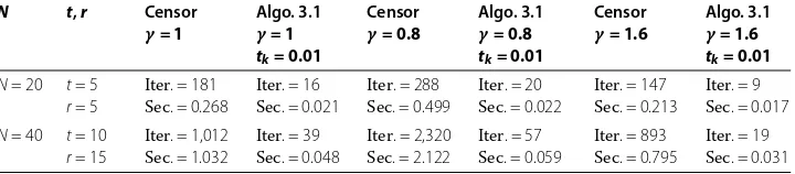
Table 2 The numerical results of Example 4.2
N t,r Censor
γ= 1
Algo. 3.1
γ= 1 tk= 0.01
Censor
γ= 0.8
Algo. 3.1
γ= 0.8 tk= 0.01
Censor
γ= 1.6
Algo. 3.1
γ= 1.6 tk= 0.01
N= 20 t= 5
r= 5
Iter. = 181
Sec. = 0.268
Iter. = 16
Sec. = 0.021
Iter. = 288
Sec. = 0.499
Iter. = 20
Sec. = 0.022
Iter. = 147
Sec. = 0.213
Iter. = 9
Sec. = 0.017
N= 40 t= 10
r= 15
Iter. = 1,012
Sec. = 1.032
Iter. = 39
Sec. = 0.048
Iter. = 2,320
Sec. = 2.122
Iter. = 57
Sec. = 0.059
Iter. = 893
Sec. = 0.795
Iter. = 19
Sec. = 0.031
Example .[] In this example, because the step is related toρ(ATA), for easy control of the spectral radius, we take diagonal matricesAandaii∈(, ) generated randomly
Ci=
x∈ N| x–di≤ri
, i= , , . . . ,t;
Qj=
x∈ N |Lj≤y≤Uj
, j= , , . . . ,r;
wherediis thecenter of the ballCi,e≤di≤e, andri∈(, ) is the radius,diandri
are all generated randomly.LjandUjare the boundary of the boxQjand are also generated
randomly, satisfying e≤Lj≤e, e≤Uj≤e. In this test, we takeeas the
initial point.
In Tables -, the results showed that for most of the initial point, the number of iter-ative steps and the CPU time of Algorithm . are obviously less than those of Censoret al.’s algorithm. Moreover, when we takeN= ,, the number of iteration steps of Algo-rithm . is only hundreds of times. The numerical results also show that for large scale problems Algorithm . converges faster than Censor’s algorithm.
5 Conclusion
The multiple-set split feasibility problem arises in many practical applications in the real world. This paper constructed a new searching direction, which is not the gradient of a corresponding function. This different direction results in a very different way of analysis. And preliminary numerical results show that our new method converges faster, and this becomes more obvious while the dimension is increasing. Finally, the theoretically analysis is based on the assumption that the solution set of the MSSFP is nonempty.
Competing interests
The authors declare that they have no competing interests.
Authors’ contributions
[image:9.595.119.479.235.314.2]Author details
1School of Management, University of Shanghai for Science and Technology, Shanghai, 200093, China.2College of
Computer Science and Technology, Henan Polytechnic University, Jiaozuo, Henan 454000, China. 3School of Physics and Chemistry, Henan Polytechnic University, Shiji Road, Jiaozuo, Henan 454000, China.
Acknowledgements
This work was supported by Natural Science Foundation of Shanghai (14ZR1429200), National Science Foundation of China (11171221), National Natural Science Foundation of China (61403255), Shanghai Leading Academic Discipline Project under Grant XTKX2012, Innovation Program of Shanghai Municipal Education Commission under Grant 14YZ094, Doctoral Program Foundation of Institutions of Higher Education of China under Grant 20123120110004, Doctoral Starting Projection of the University of Shanghai for Science and Technology under Grant ID-10-303-002, and Young Teacher Training Projection Program of Shanghai for Science and Technology.
Received: 2 November 2014 Accepted: 26 January 2015
References
1. Censor, Y, Elfving, T, Kopf, N, Bortfeld, T: The multiple-sets split feasibility problem and its applications for inverse problems. Inverse Problems21, 2071-2084 (2005)
2. Censor, Y, Elfving, T: A multiprojection algorithm using Bregman projections in a product space. Numer. Algorithms8, 221-239 (1994)
3. Censor, Y, Bortfel, D, Martin, B, Trofimov, A: A unified approach for inversion problems in intensity-modulated radiation therapy. Phys. Med. Biol.51, 2353-2365 (2006)
4. Byrne, C: Iterative oblique projection onto convex sets and the split feasibility problem. Inverse Probl.18, 441-453 (2002)
5. Dang, Y, Gao, Y: The strong convergence of a KM-CQ-like algorithm for split feasibility problem. Inverse Problems27, 015007 (2011)
6. Dang, Y, Gao, Y: A perturbed projection algorithm with inertial technique for split feasibility problem. J. Appl. Math. (2012). doi:10.1155/2012/207323
7. Dang, Y, Gao, Y: An extrapolated iterative algorithm for multiple-set split feasibility problem. Abstr. Appl. Anal.2012, Article ID 149508 (2012)
8. Yang, Q: The relaxed CQ algorithm solving the split feasibility problem. Inverse Problems20, 1261-1266 (2004) 9. Xu, H: A variable Krasnosel’skii-Mann algorithm and the multiple-set split feasibility problem. Inverse Problems22,
2021-2034 (2006)
10. Masad, E, Reich, S: A note on the multiple-set split convex feasibility problem in Hilbert space. J. Nonlinear Convex Anal.8, 367-371 (2007)
11. Censor, Y, Alexander, S: On string-averaging for sparse problems and on the split common fixed point problem. Contemp. Math.513, 125-142 (2010)
12. Censor, Y, Alexander, S: The split common fixed point problem for directed operators. J. Convex Anal.16, 587-600 (2009)
13. Censor, Y, Motova, A, Segal, A: Perturbed projections and subgradient projections for the multiple-sets split feasibility problem. J. Math. Anal. Appl.327, 1244-1256 (2007)
14. Gao, Y: Piecewise smooth Lyapunov function for a nonlinear dynamical system. J. Convex Anal.19, 1009-1016 (2012) 15. Bauschke, HH, Jonathan, MB: On projection algorithms for solving convex feasibility problems. SIAM Rev.38, 367-426
(1996)
16. Bauschke, HH, Combettes, PL: Convex Analysis and Monotone Operator Theory in Hilbert Spaces. Springer, Berlin (2011)
17. Byne, C: An unified treatment of some iterative algorithms in signal processing and image reconstruction. Inverse Probl.20, 103-120 (2004)