FACTORS AFFECTING IS SUCCESS AND TECHNOLOGY ACCEPTANCE: A CASE STUDY

ISSN: 1992-8645 www.jatit.org E-ISSN: 1817-3195

6842

MODELING OF STOCK MANAGEMENT BY PARAMETRIC

MODELS ARX, ARMAX, BJ AND OE

1_{HICHAM FOURAIJI,} 2_{BANAYAD NSIRI,} 3_{BAHLOUL BENSASSI}

1, 3 _{GITIL laboratory, faculty of sciences Ain Chock Hassan II University, Casablanca Morocco}

2_{Departement of Applied Mathematics and informatics, Ecole Normale Supérieure de l’Enseignement}

Technique Mohamed V University, Rabat, Morocco

E-mail: 1_{[email protected]}

_,

ABSTRACT

In this paper, we propose a new approach to the modeling of storage systems. This method is based on the knowledge of the automatic domain, in order to construct a mathematical model that accurately formalizes the behavior of the system studied. The approach adopted for this study is the parametric identification of ARX, ARMAX, Box Jenkins and OE linear systems. The logistic system studied will be considered as a black box, which means that the input and output data of the system will be used to identify internal system parameters and propose a mathematical model.

Keywords: Warehousing system, Modeling, Identification, ARX, ARMAX, OE, BJ

1. INTRODUCTION

During last decades, the industrial companies are confronted with great changes in their environment, a world competition, a dubious market, and increasingly demanding customers. These various constraints impose a reactivity and flexibility of the companies with an aim of adapting the capacity of the systems of production to the changes of the request and the internal and/or external risks of the line productions. What requires a thorough knowledge of the characteristics of the supply chain.

Difficult to control, these systems continue to pose serious problems of design, modeling and control. Indeed, the logistic study of the systems, like any type of dynamic system, proves to be a task very difficult to realize, and very often requires that one has mathematical models of these systems. These models can be deduced directly from the physical laws which govern the behavior of the system, but it is often impossible to obtain a knowledge a priori supplements and precise of all the parameters of the model.

In this case, to refine and specify this knowledge, one resorts to a behavioral model

estimated starting from the input-outputs observed of the system. This refers to the identification approach, which is the set of methodologies for the mathematical modeling of systems, based to real measurements from the process [1].

6843 realized a simulation platform and they also proposed pilotage principles of integrated logistics chain [4]. BROHEE and al. used hybrid Petri networks to offer an offline simulation approach that supports multiple constraints (control change, time among developments, friction ....). The originality of their work lies in the fact that they proposed a simulation of continuous part production and the study of interactions between the continuous model and discrete data exchanged with the control part. This approach allows simulating and controlling the system without using the actual operative part, these contributions are based on a schematic modeling, without interested to the internal parameters of the system studied [5]. H.SARIR and al. presented a modeling approach and regulatory work in progress stocks in the macroscopic analogy of production lines with the control model of a hydraulic tank. They used the concepts of automatic control for monitoring and mastering of in-process inventories [6]. H.SARIR and al. who also presented a model of a production line using the behavioral identification in discrete time by the transfer functions, they used the PEM algorithm for the construction of models and the simulation was performed on the graphical interface (IDENT) in MATLAB© [7]. K.TAMANI and al. proposed a process for controlling product flow, where they broke down the system studied as basic production modules. They proposed thereafter, the control of flow through each output module and supervision which was based on fuzzy logic [8].

This literature study, we show that the logistics systems today are a focus for scientific research in the field of modeling.

Modeling approaches are many and varied, but it appears that the methods of analysis and production system design combining different approaches are preferred. Indeed the latter bring an ease of analysis or increased use or opportunities to put in simplified work.

We found that modeling logistics systems, based on parametric models is rarely used, and that much of the work focuses on the schematic or analytical modeling (Petri nets, UML ....), while parametric and behavioral modeling is rarely discussed.

This article propose a method for modeling logistics systems based on parametric models.

2. IDENTIFICATION METHOD

The purpose of any modeling system is to build a model, that is to say, a mathematical representation of its operation. Dynamical systems, we are

interested in this work, are at the heart of the supply chain (storage system and storage). It is often necessary to build a model to understand, simulate, controlled and steered these systems.

When modeling a process, two approaches are possible:

The first is to build a knowledge model. Designing knowledge models stems from a physical analysis of phenomena involved in the system; when necessary, the system is broken down into simpler components studied, for which already has a proven knowledge model. Experimental data are then used, first to numerically estimate the values of model parameters, then obtained to validate the model. In particular, scientific research essential purpose the construction of models of this type, which allow not only to understand but also to extrapolate the behavior of any system.

The second approach is to build a model type "black box". Specifically, the aim is a mathematical expression that reflects faithfully the behavior "input-output" system studied in an area of operation defined use. The parameters usually have no physical meaning. The numerical estimation of these parameters based primarily on a set of experimental observations that are available on the system; The models 'black box' is usually in times of economic calculation. Their validity is limited to an operating range determined by the set of measured input-output, while that of knowledge models is determined by the accuracy of assumptions and relevance of the approximations made in the physical analysis of phenomena and equation of their layout. As part of the design of "black box" models of dynamic system, the parametric models are an excellent candidate that is typically used to approximate the dynamic behavior of the system in a satisfactory manner.

In this work, we focus on the development of models of the type "black box" of dynamical systems. We only consider the case of stationary systems, that is to say, such as the laws that govern their behavior does not change over time. The models we consider are discrete-time models.

ISSN: 1992-8645 www.jatit.org E-ISSN: 1817-3195

6844 calculations quickly. In addition, their design is closely related to the particular process that is desired to be modeled, and the knowledge available on the physical thereof.

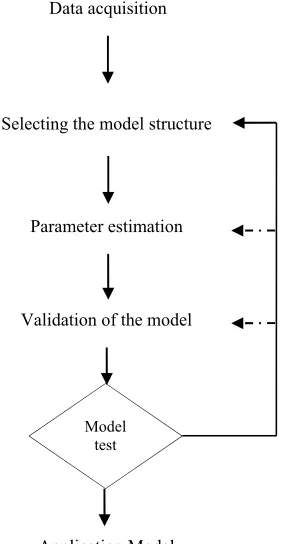
A mathematical model is always an approximation of the real system. In practice, system complexity, limited prior knowledge of the system and incomplete observed data prevents an accurate mathematical description of the system. However, even if we have a complete knowledge of the system and enough data, an accurate description often is not desirable because the model would become too complex to be used in an application. Therefore, identification of the system is regarded as an approximate model for a specific application on the basis of the observed data and knowledge of the prior system. The identification procedure in order to reach an appropriate mathematical model of the system, is described in detail in Figure 1.

2.1 The acquisition of Data set

The first step in the identification process is the acquisition of data, this step is very important, why we must choose the data that will be used to model the system, for that must use data covering the entire range system operating in normal conditions.

the input and output data should be divided into two data sets, the first data portion to estimate while the second part of data validation purposes.

2.2 Choosing the model structure

The parametric model describes a system in terms of differential transfer function. There are few models of structures that can be used to represent certain system. In general, the structure of the parametric model used is based on the equation (1) [9].

𝑦 𝑡 𝑞 𝐺 𝑞 𝑢 𝑡 𝐻 𝑞 𝑒 𝑡

Where q G q u t represents the output without disturbance, and H q e t designates the disturbance [1]. q is the argument of G q and

H q , it is the offset operator, which is equivalent to q represented by q and can be demonstrated by q x t x t 1 , nk is the delay time in the sampling time between the input and the output of the process. In modeling process, always nk 1 to ensure causality [2].

Four linear models are considered in this study. These models are ARX, ARMAX, BJ, and OE model. In this article, the studied system is a multi inputs single-output (MISO).

2.2.1 ARX model

The structure of the ARX model is given by:

y t a y t 1 . . . a y t n b u t 1 …

b u t n n 1 e t

when n and n are the orders of the ARX model, (n is the number of poles and n is the number of zeros plus 1), n is the delay (number of samples of the input that occur before the input affects the output, also called the dead time in the system), y t is output as a function of time, u t is the input of system, is function of time, and e t is the term that represents the disturbance in the form of white noise.

We present this function with compact form as (1) :

y t q u t e t

The polynomials A q and B q are given by :

A q 1 a q . . . a q B q b b q . . . b q

A q and B q represent the dynamic system,

q is the delay operator, this description of q is equivalent to the transformed z [10].

Data acquisition

Validation of the model Parameter estimation

Application Model Selecting the model structure

Model test

Figure 1 : identification process

(1)

(2)

(3)

(4)

6845

a … … a and b … … b are the parameters of the polynomials. The flow of the signal can be represented by the following figure:

2.2.2 ARMAX model

The structure of the ARMAX model is given by:

y t a y t 1 … a y t n b u t n … b u t n n 1 c e t 1 . . . c e t n e t

when n and n are the orders of the ARMAX model, (n is the number of poles and n is the number of zeros plus 1), n is the number of zeroes of disturbance term. n is the delay (number of samples of the input that occur before the input affects the output, also called the dead time in the system), y t is output as a function of time, u t is the input of system, is function of time, and e t is the term that represents the disturbance in the form of white noise.

y t q u t e t

The polynomialsA q , B q and C q are given by:

A q 1 a q . . . a q B q b b q . . . b q C q 1 c q . . . c q

A q and B q represent the dynamic system,

C q represent the model of distrubance, q is the delay operator, this description of q is equivalent to the transformed z

[10], a … … a b … … b and c … … c are the parameters of the polynomials. The flow of the signal can be represented by the following figure:

2.2.3 OE model

The structure of the OE model is given by:

y t f y t 1 … f y t n b u t n …

b u t n n 1 v t

when n and n are the orders of the OE model, (n is the number of poles and n is the number of zeros plus 1. n is the delay (number of samples of the input that occur before the input affects the output, also called the dead time in the system),

y t is output as a function of time, u t is the input of system, is function of time, and v t is the term that represents the disturbance.

y t q u t v t

The polynomials F q and B q are given by :

F q 1 f q . . . f q

Figure.2: The ARX model structure

𝐵

𝐴 𝑦 𝑡

𝑢 𝑡

𝑒 𝑡

𝑢 𝑡 𝐵

𝐴

1 𝐴

Figure.3: the ARMAX model structure

𝐵

𝐴 𝑦 𝑡

𝑢 𝑡

𝑒 𝑡

𝑢 𝑡 𝐵

𝐴

𝐶 𝐴

Figure.4: the OE model structure

𝐵

𝐹 𝑦 𝑡

𝑢 𝑡

𝑣 𝑡

𝑢 𝑡 𝐵

𝐹 (6)

(7)

(8)

(10)

ISSN: 1992-8645 www.jatit.org E-ISSN: 1817-3195

6846 (13)

(14)

(16)

(17)

B q b b q . . . b q

F q and B q represent the dynamic system,

q is the delay operator, this description of q is equivalent to the transformed z [10], f … … f and

b … … b are the parameters of the polynomials. The flow of the signal can be represented by the following figure:

2.2.4 Box Jenkins model

BJ model belongs to the class of output error models, it is a model OE with additional degrees of freedom for the noise model while the OE model assumes a white additive disturbance at the output of the process, allows the BJ modeling of any disturbance. It can be generated by filtering white noise through a linear filter with numerator and

denominator arbitrary.

BJ model is illustrated in Figure 5 by:

y t q B q F q u t

C q D q v t

The polynomials F q and B q are given by:

F q 1 f q . . . f q B q b b q . . . b q C q 1 c q . . . c q D q 1 df q . . . d q

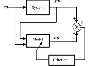
2.3 parameter estimation

It is choosing an estimation algorithm or a criterion to be minimized. For parametric models, we use least squares algorithm to minimize prediction error Ɛ between the estimated output

𝑦 𝑡 and real output y t Figure 2 illustrate the estimation model adopted for this study.

Parameter estimation by least squares (MC) is the approach most commonly used for identification systems [10]. Introducing a vector regressionφ k , equation (1) can be rewritten as a linear regression:

y k φ k θ ε k

Where φ k is the observation vector:

φ k y k 1 , … , y k na , u k nk , … , u k nk nb 1 (15)

The criterion function used for the least squares estimation is given by:

V θ 1

N y k φ k θ ²

Minimizing the function of the test, we can get an estimate of θ:

θ argmin V θ

Once a series of input-output information is given, the model parameters are estimated using the least square method. In addition, the recursive modeling technique is a fast technique for estimating the model parameters, after each sampling of a data set. Thus, in this study, the least squares method and the recursive algorithm with forgetting factor used for the identification of line parameters of the model presented in (9).

This method gives an estimate of parameter model studied minimizing recursively (MC) defined by the criterion (14).

2.4 Model validation

Model validation is the final step is an obligatory step in deciding whether the identified model is accepted or not. The purpose of model validation is

- u(t)

y(t)

x(t)

+ Ɛ

System

Model

Criterion

Figure 6: Identification principle based on the prediction error

Figure.5: The Box Jenkins model structure

𝐵

𝐹 𝑦 𝑡

𝑢 𝑡

𝑣 𝑡

𝑢 𝑡 𝐵

𝐹

𝐶 𝐷

6847 (18)

(19) to check whether the model identified meet the requirement of modeling for a particular application. In achieving good estimated model, it is necessary to distinguish between the lack of fit between the model and the data due to random processes and, due to the lack of model complexity. In most statistical tools, measuring the fit of a model is determined by the coefficient of determination R2 _[12].

The R2 _{is given by:}

R 1

0 R 1

The RMSE (root mean square error) is used to evaluate the performance prediction of a preacher, like the prediction accuracy increases, the mean square error decreases [12].

RMSE 1

N ỹ y

3. STUDY CASE

To better understand this method of identification and verify its effectiveness, we propose to model the stock level of a distribution company, that stock is divided into two families, high turnover and average rotation, for items low rotation, are not a focus for this study.

The warehouse of this company is managed according to a procurement policy, receptions are based on estimates prepared by the purchase and supply department, while orders are random (according to customer demand), which requires good management stock never dropped out or have a costly overstock. The procurement method followed for the management of this warehouse is an anticipation of demand (forecasts are not included in this study).

The stock will be considered a MIMO (multiple input, single output) or entries are the receipts and shipments while the output is the stock level for this study were asked a few assumptions:

We have considered the stock as an invariant system in time (the stock characteristics do not change over time).

We took the time unit equal to one day.

After receiving the items are entered into the management system and immediately appear on the system.

In the first place we consider the stock as a black box with two inputs and one output (entries are: corresponds to the currently tuned merchandise, and represents the daily flow of shipping, while the output is the level of stock holding ).

Figure.7: representation of the system as "black box"

The input and output data were extracted from the warehouse information system. These data are used to model the stock by comparing models of structures ARX, ARMAX, OE and Box Jenkins [12].

The data is divided into two parts. The first part is used to determine the model of the system and the second is applied for the purpose of validating the model.

3.1. FOR FAST MOVING PRODUCTS:

Figure.8 :representation of inputs and outputs

Stock

u t

y t

u t

0 20 40 60 80 100 120 140 160 180

-2000 -1000 0 1000 2000 3000 4000

N

iv

eau

de

st

ock

la variation du niveau de stock en fonction des réceptions

0 20 40 60 80 100 120 140 160 180

Time -2000

-1000 0 1000 2000 3000 4000

le

s

ré

cept

ions

0 20 40 60 80 100 120 140 160 180 200

-2000 -1000 0 1000 2000 3000 4000

n

iv

eau

d

e

st

ock

la variation du niveau de stock en fonction des expéditions

0 20 40 60 80 100 120 140 160 180 200

Time

-100 -50 0 50 100 150 200

le

s

exp

éd

iti

on

ISSN: 1992-8645 www.jatit.org E-ISSN: 1817-3195

6848 Figure 8 shows the change in the level of stock based on monthly shipments and receptions for a product with high rotation.

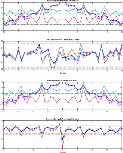
Figures 9, 10, 11, 12 representing simulation models found with parametric models, we find that the OE and BJ models give satisfactory results; the best fit is that of the OE model (fewer parameters and the best fit)

At the end of ensuring the results found previously, we conducted a correlation test for the 4 models, these results confirm that the best model for items with a high turnover is the OE.

The table below shows the settings and information for each model (the number of parameters, the percentage adjustment and FPE).

0 20 40 60 80 100 120 140 160 180 200

Time(days) -2000

-1500 -1000 -500 0 500 1000 1500 2000

2500 Measured and simulated model output

OE model : 93,11%

real data

-20 -15 -10 -5 0 5 10 15 20

-0.4 -0.2 0 0.2 0.4

0.6 Autocorrelation of residuals for output y1

-20 -15 -10 -5 0 5 10 15 20

Samples

-0.2 -0.1 0 0.1

0.2 Cross corr for input u2 and output y1 resids

-20 -15 -10 -5 0 5 10 15 20

-0.4 -0.2 0 0.2 0.4

0.6 Autocorrelation of residuals for output y1

-20 -15 -10 -5 0 5 10 15 20

Samples

-1 -0.5 0

0.5 Cross corr for input u1 and output y1 resids

0 20 40 60 80 100 120 140 160 180 200

Time (days) -2000

-1500 -1000 -500 0 500 1000 1500 2000

2500 Measured and simulated model output

ARX Model 80,32% real data

Figure 9: the comparison of the actual stock level and the estimated stock level for the ARX model

0 20 40 60 80 100 120 140 160 180 200

Time(days) -2000

-1500 -1000 -500 0 500 1000 1500 2000

2500 Measured and simulated model output

ARMAX model 72,54% real data

Figure 10: the comparison of the actual stock level and the estimated stock level for the ARMAX model

Figure 11: the comparison of the actual stock level and the estimated stock level for the OE model

0 20 40 60 80 100 120 140 160 180 200

Time(days) -2000

-1500 -1000 -500 0 500 1000 1500 2000

2500 Measured and simulated model output

BJ model : 88,43%

real data

Figure 12: the comparison of the actual stock level and the estimated stock level for the BJ model

6849

Model Best fit % FPE Polynomial equation

ARX 80,32% 2255

A z 1 1,003Z 0,01241Z 0,001952Z

B z 0,2954Z

B z 0,9856

ARMA

X 72,54% 2356

A z 1 1,509Z 0,04706Z 0,552Z 0,00639Z

B z 0,2786Z 0,5027Z 0,007711Z

B z 0,9842 0,4906Z 0,5725Z

C z 1 1,19Z 0,1903Z

OE 93,11% 2081

B z 0,3264Z 0,3748Z 0,1426Z

B z 0,9982 0,9306Z

F z 1 0,008749Z 0,9447Z

F z 1 1,931Z 0,9314Z

BJ 88,43% 2056

B z 0,3433Z 0,4435Z 0,1853Z

B z 0,9881 0,8789Z

C z 1 1,137Z 0,179Z

D z 1 0,4123Z 0,3263Z

F z 1 1,88Z 0,8898Z

F z 1 1,891Z 0,8935Z

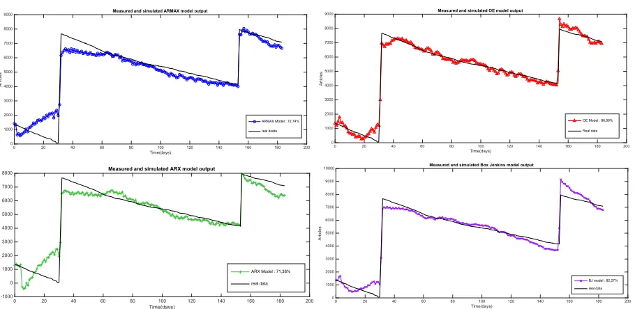
3.2 For medium rotation products:

Figures 14 shows the change in the level of stock based on monthly shipments and receptions for a product with high rotation.

Figures 15 representing simulation models found with parametric models, we find that the OE and BJ models give satisfactory results, the best fit is that of the OE model (fewer parameters and the best fit).

0 20 40 60 80 100 120 140 160 180

0

2000 4000 6000 8000

in

ve

n

to

ry

le

ve

l

Input and output signals

0 20 40 60 80 100 120 140 160 180

Time(days) 0

50 100 150

or

der

s

hi

pped

0 20 40 60 80 100 120 140 160 180 200

0

2000 4000 6000 8000

in

vent

or

y

le

ve

l

Input and output signals

0 20 40 60 80 100 120 140 160 180 200

Time(days) 0

1000 2000 3000 4000

re

ce

pt

io

n

ISSN: 1992-8645 www.jatit.org E-ISSN: 1817-3195

6850 To ensure the results found previously, we conducted a correlation test for the 4 models, these results confirm that the best model for items to medium rotation is the OE.

The table below shows the settings and information for each model (the number of parameters, the percentage adjustment and FPE).

-20 -15 -10 -5 0 5 10 15 20

-0.5

0 0.5

1 Autocorrelation of residuals for output y1

-20 -15 -10 -5 0 5 10 15 20

Samples -0.2

-0.1 0 0.1

0.2 Cross corr for input u2 and output y1 resids

-20 -15 -10 -5 0 5 10 15 20

-0.5

0 0.5

1 Autocorrelation of residuals for output y1

-20 -15 -10 -5 0 5 10 15 20

Samples -0.2

0 0.2 0.4 0.6

0.8 Cross corr for input u1 and output y1 resids

Figure 16: result of the correlation tests of the four models

0 20 40 60 80 100 120 140 160 180 200

Time(days) -1000

0 1000 2000 3000 4000 5000 6000 7000 8000

art

ic

les

Measured and simulated ARX model output

ARX Model : 71,38%

real data

0 20 40 60 80 100 120 140 160 180 200

Time(days) 0

1000 2000 3000 4000 5000 6000 7000 8000 9000

Ar

tic

le

s

Measured and simulated ARMAX model output

ARMAX Model : 72,74% real dsata

0 20 40 60 80 100 120 140 160 180 200

Time(days) 0

1000 2000 3000 4000 5000 6000 7000 8000 9000

Ar

tic

le

s

Measured and simulated OE model output

OE Model : 86,89%

Real data

0 20 40 60 80 100 120 140 160 180 200

Time(days) 0

1000 2000 3000 4000 5000 6000 7000 8000 9000 10000

Arti

cl

es

Measured and simulated Box Jenkins model output

BJ model : 82,27% real data

6851

Model Best fit % FPE Polynomial equation

ARX 71,38% 6897.104

A z 1 1,102Z 0,1436Z 0,02692Z 0,123Z

0,1096Z 0,03473Z

B z 09795Z 0,08847Z

B z 4,133Z 6,349Z 3,324Z 0,4717Z

4,732Z

ARMAX 72,74% 2356

A z 1 0,9235Z 0,1506Z ,089Z

B z 0,957Z 0,09434Z

B z 4,244Z 6,226Z

C z 1 0,2277Z 0,1233Z 0,2191Z

OE 88,89% 2081

B z 0,3264Z 0,3748Z 0,1426Z

B z 0,9982 0,9306Z

F z 1 0,008749Z 0,9447Z

F z 1 1,931Z 0,9314Z

BJ 82,89% 2056

B z 0,3433Z 0,4435Z 0,1853Z

B z 0,9881 0,8789Z

C z 1 1,137Z 0,179Z

D z 1 0,4123Z 0,3263Z

F z 1 1,88Z 0,8898Z

F z 1 1,891Z 0,8935Z

4. CONCLUSION

ISSN: 1992-8645 www.jatit.org E-ISSN: 1817-3195

6852

REFRENCES:

[1] L. Ljung, System Identification: Theory for the User, 2nd Ed. New Jersey: Prentice Hall PTR, 1999

[2] Karim Labadi and al. “Modeling and performance evaluation of supply chains using batch deterministic and stochastic Petri nets”, IEEE Transactions on Automation Science and Engineering, 11 April, 2005, pp. 132-144. [3] N.Smata, C.Tolba, D.Boudebous,

S.Benmansour, J. Boukachour, “ Modélisation de la chaîne logistique en utilisant les réseaux de Pétri continus ”, 9e Congrès International de Génie Industriel, Canada, October, 2011. [4] F. Petitjean, P. Charpentier, J-Y. Bron , A.

Villeminot, Modélisation globale de la chaine logistique d’un con structeur automobile, "eSTA" :La Revue électronique Sciences et Technologies de l’Automatique, N1 Spécial JD -JNMACS’ 07 2ème partie, 2008.

[5] B. Rohee, B. Riera, V. Carre-Menetrier, JM. Roussel, outil d’aide à l’élaboration de modèle hybride de simulation pour les systèmes manufacturier, "Journées doctorales du GDR MACS (JD-MACS'07), Reims, France , 2007. [6] H.Sarir, L’intégration d’un module d’a ide à la

décision (contrôle de flux entrée-sortie) basé sur le modèle régulation de niveau dans le système MES (Manufacturing Execution System, Colloque SIL–Concours GIL Award, (Déc. 2011).

[7] H. Sarir, B.Bensassi, Modélisation d’une ligne de fabrication d’un sous ensemble de l’inverseur de pousse par la méthode d’identification, IJAIEM : international journal of application or innovation in engineering and management, ISSN 2319 – 4847 Volume 2, Issue 6, (Juin 2013).

[8] K.Tamani, Développement d’une méthodologie de pilotage intelligent par régulation de flux adaptée aux systèmes de production, thèse de doctorat, université de Savoie, France, (Déc.2008).

[9] Z.M.Yusoff, Z.Muhammad, M.H.F. Rahiman, M.N. Taib, ARX Modeling for Down-Flowing Steam Distillation System, IEEE 8th International Colloquium on Signal Processing and its Application, 2012.

[10] Z.Muhammad, Z.M.Yusoff, M.H.F. Rahiman, M.N. Taib, Modeling of Steam Distillation Pot with ARX Model, IEEE 8th International

Colloquium on Signal Processing and its Application, 2012.

[11] K. Ramesh, N. Aziz and S.R. Abd Shukor, “Nonlinear Identification of Wavenet Based Hammerstein Model – Case Study on High P urity Distillation Column”, Journal of Applied Sciences Research, 3(11): 1500-1508, 2007. [12] H. Akaike, “A new look at the st atistical model

identification”, [13] IEEE Transactions on Automatic Control 19 (1974) 716– 723.