An Analysis of Convolutional Neural Networks for Image Recognition

2017 2nd International Conference on Computational Modeling, Simulation and Applied Mathematics (CMSAM 2017) ISBN: 978-1-60595-499-8

An Analysis of Convolutional Neural Networks for Image Recognition

Jun HE

, Yue LIU, Shuai LI and Jin-ming SHEN

College of Information & Engineering, Nanchang University, Nanchang, China *Corresponding author

Keywords: Convolution neural network, Local receptive fields, Image recognition.

Abstract. At present, Convolution Neural Network (CNN) has been widely applied to image recognition. Most of the researches focus on the CNN algorithm research, but there are few studies on the impact of the CNN’s parameters. In view of this situation, this paper focuses on the influence of each parameter on the experimental results. Through a series of Handwritten-Font-Recognition experiments using Convolution Neural Network, the relations between these parameters (e.g. the depths of CNN, the step sizes) in these modes and the influence of different parameter setting are preliminary grasped, which provides a reference for the study of CNN. We aim to help readers understand the relevant work methods and ideas by these experiments.

Introduction

At present, there are many algorithms used for image recognition, e.g. Gabor filter, support vector machine (SVM), genetic algorithm, neural network algorithm. In the traditional image recognition, it is mainly to extract the feature points from the image, and then use the feature to identify the image, but the process is more complicated and easily lead to the accumulation of error. In recent years, the focus of image recognition has begun to shift to deep learning.

In 2006, Hinton et al. [1] presented the concept of "deep learning" in "Science". The main points are as follows: (1) The artificial neural network with multiple hidden layers has excellent characteristic learning ability. (2) Depth neural network can solve the problem of training effectively through greedy layer-wise pre training [8]. Recently, with the emergence of large-scale database and the rapid development of computer hardware, this makes it possible for deep neural networks to obtain high-level features and large data processing, and greatly improves the accuracy of the experiment. CNN is a kind of artificial neural network, which has become a hotspot in the field of speech analysis and image recognition [2, 3, 4], which has a good recognition effect for translational, scaled, skew, or altogether deformed images. It can take the original image as input, which avoids the complicated feature extraction and data reconstruction process in the traditional recognition algorithm. LeNet ⁃5 is a type of traditional convolutional neural network proposed by Yann Lecun et al [4]. It combines feature extraction and recognition to select and optimize features through continuous back propagation, transforming feature extraction into a self-learning process, and finding the best performance of classification by this method. The main idea of CNN is local receptive fields, shared weights, BP algorithms[4, 5, 6].The structure consists of the input layer, convolution layers, pooling layers and the full connection layer.

This paper focuses on LeNet's theory, and uses LeNet-5 for handwritten font experiments to analyze the effect of parameters on CNN.

Theoretical Analysis

Main Idea

hidden layer, with a same weight parameter W. The local perception fields will move from left to right, from top to bottom and each move distance is called step size. This map from the input layer to the hidden layer is called feature map.

Shared weights: Each neuron in the hidden layer is connected to a 5 x 5 local image, so there are 25 weight parameters. In order to reduce the amount of data calculations, according to the relevance of the characteristics, we let the remaining neurons share these 25 weight parameters, that is, regardless of the number of hidden neurons at this time, the parameters that we need to train are just 25 weight parameters. The weight of the feature map is called shared weight. The Shared-weights method reduces the complexity of the network model, reducing the number of weights.

Back Propagation: CNN also uses the back propagation algorithm to update the parameters of each layer, including the weight of each layer, and the offset parameters, which is also widely used in deep learning network [7]. Unlike standard BP algorithm [11], the neurons of two adjacent layers are not fully connected, but partly connected. In the back propagation process, the weight matrix is adjusted by gradient descent, and the parameters of each layer that have been initialized will be update according to the difference between the actual output and the corresponding ideal output.

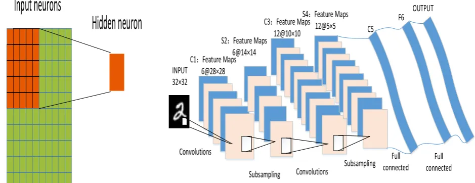
Input neurons

Hidden neuron

INPUT 32×32

C1：Feature Maps 6@28×28

C3：Feature Maps 12@10×10 S2：Feature Maps

6@14×14

S4：Feature Maps

12@5×5 F6

OUTPUT

Convolutions Subsampling

Full connected Full

connected C5

Convolutions

Subsampling

Figure 1. Local receptive fields (Left) and the LeNet-5 structure (Right).

The Structure of LeNet-5

Experiments were performed using LeNet-5 and the number of convolutions and pooled layers of the network was changed for handwritten font experiments. In this section, we will briefly introduce the structure of LeNet-5 as shown in Fig. 1(Right).

Convolution Layer

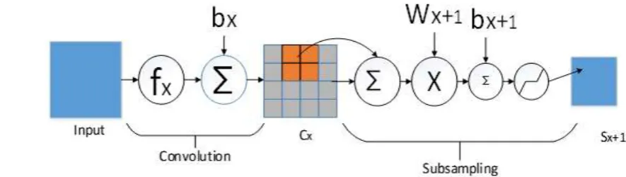
The convolution layers are the feature extraction layers. Each convolution layer is composed of multiple feature maps, which is composed of many neurons. CNN's convolution layer extracts the different characteristics of the input by convolution kernel that is a weight matrix (such as a 3 × 3 or 5 × 5 matrix for a two-dimensional image). The first layer of the convolution layer extracts lower-level features such as edges, lines, corners, and the higher layer of the convolution layer to extract more advanced features. Convolution process is shown in Fig. 2. We can calculate the size of the output feature [4] by

N = (W − F + 2P)/S+1 (1)

Figure 2. Convolution and subsampling process.

Pooling Layer

The pooling layer uses the image local correlation to sub-sample the image, which can reduce the amount of data processing while preserving useful information. The pooling process is shown in Fig.2. A new pixels that is obtained by summing the 4 pixels (2 × 2) of each field of input maps. We can get Sx + 1 as Eq.2 [4] show

. (2) is the feature map of l-1 layer, pool（*） is the pooling function, is the weight of

pooling layer(l), is the bias of pooling layer(l).

The pooling types (pooling function) include mean-pooling, max-pooling. Mean-pooling takes the mean value of each sub-region as the result, and max-pooling takes the maximum value of each sub-region as the result. Boureau et al. [9] compared the two methods. It was found that when the classifier uses a linear classifier such as linear SVM, the maximum pooling method achieves a better classification than the mean pool performance. In addition, there are random pool, mixed pool, space pyramid pool, pooling and other pooling methods [8].

Full connection Layer

In full connection layer, all the two-dimensional image of the feature map will be converted into a one-dimensional feature as a fully connected network input. The output will be sent to classifier, which can be obtained by summing the input weight and passing the activation function [4, 9].

xl=f(wlxl-1+bl). (4)

xlis the feature map of l layer, f（*） is the activation function, xl-1 is the feature map of l layer,

wl is the weight of pooling layer(l), bl is the bias of layer(l).

Experiments and Analysis

In this paper, the effects of different parameters on the results are discussed by contrast experiments. We ran these experiments by using Matlab R2016a under Windows7 platform.

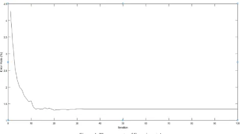
In experiment A, we use MNIST dataset [12] and LeNet-5 as shown in Fig.1. There are 60000 samples for training, and 1000 samples for test, whose size is 28 × 28. To adapt to LeNet-5, all data normalized to 32 ×32. Although the partial data is transformed by translation, rotation, scale, and skew of the original image, the experiment can still have a good recognition rate. Due to the large amount of data, we carried out batch training method, and the number of each batch is 50. The number of iterations is 100, and the activation function is Sigmoid. As shown in Fig.4, when the iterations reaches about 10 times, the error rate tends to be stable. In other experiments in addition to variable and iteration number (20times), the rest has the same parameters as experiment A.

Figure 4. The error rate of Experiment A.

As shown in Table 1, we set five groups of learning rates respectively and observed its error rate on the experiment B. We can see a suitable learning rate can reduce the error rate. The size of batches also has some effect on the experiment C. It shows that the smaller the error rate of each batch.

Table 1. The error rate (%) of experiments B and C.

It can be seen from Table 2 that too few convolution and pooling layers can lead to low recognition rates, too much is not significantly improved to recognition rate.

Table 2. The error rate based on different number of layers.

Case Convolution layer Pooling layers Iteration Time (s)

Error rate (%) Number Size Number Size

1 2 5 ×5 1 2 ×2 20 519 6.14

2(LeNet-5) 3 5 ×5 2 2 ×2 20 8147 1.31

3 4 5 ×5 3 2 ×2 20 23241 1.15

Iteration Learning Rate Batch Size

Conclusion

After a series of experiments, we can infer that the improper parameters include learning rates, the number of layer and the size of the batches will result in a lower recognition rate or more time-consuming. We can also get the excellent characteristics of CNN in image recognition. First, experiments fully show CNN has some degree of translation invariance to the input local transform. Second, the whole classification process is automatic, and CNN can take the original image as the input of network directly, avoiding the manual extraction of features that would lead to the accumulation of errors. Third, using weight sharing to reduce the amount of data, this makes it possible that the experiment was carried out under poor hardware. Finally, the deeper the depth, the better the performance of the model, the more time-consuming.

Now CNN still has a lot of work to be further improved: Future work should likely include looking at the combination of other visual recognition models and the optimal network structure. For a particular task, the parameters of network structure, such as the optimal receptive field size, the number of convolution layers and the number of learning rates, are still difficult to determine.

Acknowledgement

This research was financially supported by the National Science Foundation of China (grant No. 61463034).

References

[1] Hinton, G. E., & Salakhutdinov, R. R. (2006). Reducing the dimensionality of data with neural networks, J. Science, 313(5786), 504.

[2] He, Kaiming, et al. "Deep Residual Learning for Image Recognition." Computer Vision and Pattern Recognition IEEE, 2016:770-778.

[3] Bouvrie, Jake. "Notes on Convolutional Neural Networks." J. Neural Nets (2006).

[4] Lécun, Yann, et al. "Gradient-based learning applied to document recognition." Proceedings of the IEEE 86.11(1998):2278-2324.

[5] Erhan D, Bengio Y, Courville A, et al. Why does unsupervised pre-training help deep learning? J. Journal of Machine Learning Research, 2010, 11(3):625-650.

[6] Bengio, Yoshua, et al. "Greedy layer-wise training of deep networks." International Conference on Neural Information Processing Systems MIT Press, 2006:153-160.

[7] Bengio Y. Learning deep architectures for AI. J. Foundations and Trends in Machine Learning, 2009, 2( 1) :1 -127.

[8] Boureau, Y Lan, J. Ponce, and Y. Lecun. "A Theoretical Analysis of Feature Pooling in Visual Recognition." International Conference on Machine Learning DBLP, 2010:111-118.

[9] Zhou, Fei Yan, L. P. Jin, and J. Dong. "Review of Convolutional Neural Network." J. Chinese Journal of Computers (2017).

[10] Chu, Joseph Lin, and A. Krzyżak. "Analysis of Feature Maps Selection in Supervised Learning Using Convolutional Neural Networks." Canadian Conference on Artificial Intelligence Springer International Publishing, 2014:59-70.

[11] Duda R O, Hart P E, Stork D G[Author], Li Hong-Dong, Yao Tian-Xiang [Translator]. Pattern Classification. Beijing: China Machine Press, 2003.