A Growth Perspective on Foreign Reserve Accumulation

Munich Personal RePEc Archive

A Growth Perspective on Foreign

Reserve Accumulation

Cheng, Gong

Banque de France, Sciences Po

9 December 2011

Online at

https://mpra.ub.uni-muenchen.de/46668/

A Growth Perspective on Foreign Reserve

Accumulation

Gong Cheng

March 2013

Abstract

Based on a dynamic open-economy macroeconomic model, this paper aims at un-derstanding the contribution of domestic financial under-development to foreign reserve accumulation in some emerging market economies, especially in China. It is argued that foreign reserve accumulation is a consequence of a growth strategy induced by strong capital investment in a financially constrained economy. It is further proved using a Ramsey problem that purchasing international reserves is a welfare-improving policy in terms of production efficiency gains when the domes-tic economy faces two sources of frictions: credit constraint and capital controls. In fact, when domestic firms are occasionally credit-constrained and they do not have a direct access to international financial market, they need domestic saving instruments to increase their retained earnings so that they can sufficiently invest in capital. The central bank/government plays the role of financial intermediary and provides domestic firms with a liquid public bond, thus relaxing the domestic credit constraint. The proceeds of domestic public bonds are then invested abroad due to the limited scope of domestic financial market and a depressed domestic interest rate, leading to foreign reserve stockpiling. The speed of foreign reserve accumula-tion will slow down with the domestic financial deepening and the development of the domestic financial market.

JEL Classification: F41, F43

Keywords: Foreign reserves, capital controls, credit constraints, domestic savings, capital investment, economic growth, Chinese economy

∗_{Sciences Po and Banque de France. [email protected]}

†_{I thank Philippe Martin for his decisive guidance and supervision. I am grateful to Barry Eichengreen,}

1

Introduction

1.1

Research background

Over the last decade, we observe a surge in foreign reserve accumulation throughout

the world and in particular in emerging market economies. The latter became the main

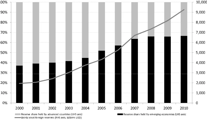
reserve holders, taking over the place of advanced countries around 2005. As Figure

1 shows, the share of foreign reserves held by emerging and developing economies has

doubled in eight years since 2000, rising from 33% to 67% of total foreign reserves in the

world.

Figure 1: Evolution of the world reserves

Facing this trend of rapid accumulation of foreign reserves in the last decade, a renewed

literature revived the debate regarding the determinants of the demand for foreign assets

and the reserve adequacy ratio. Since very recently, there seems to be a consensus deeming

that the motives of holding foreign reserves can be time-varying and specific to individual

countries or country groups. An empirical paper by Ghosh et al. (2012) and a report of

the Independent Evaluation Office (IEO) of the International Monetary Fund (IMF)

confirmed this broad view.

Evidence has shown that countries accumulate reserves for many reasons that

evolve over time. Reserve adequacy assessments and advice therefore need to

rely on a broad range of indicators which should be adjusted when

circum-stances change (IEO (2012)).

In this paper, I propose a general equilibrium model to analyze a particular factor,the

under-development of the domestic financial market, which may motivate a central bank

to purchase foreign assets. Despite the extensive academic and policy debates with regard

to international reserves, a theoretical model on the relationship between financial market

under-development and reserve accumulation remains elusive. My analysis is based on

three facts that we observe in the data.

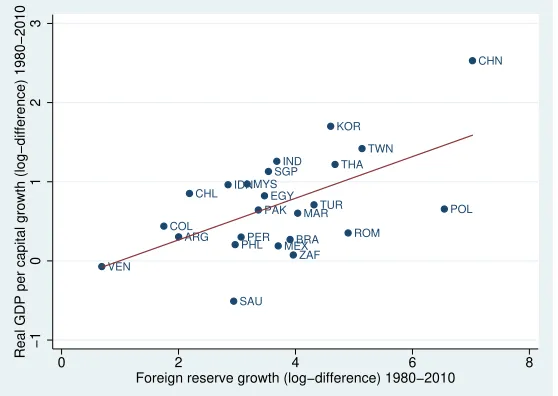
Fact 1 Emerging market economies which have accumulated a large stock of foreign

assets are those which have experienced a fast economic growth.

Figure 2 shows a clear positive relationship between the average growth rate of real

GDP per capita and that of foreign reserve stocks between 1980 and 2010 for 24 emerging

economies. ARG BRA CHL CHN COL EGY IND IDN KOR MYS MEX MAR PAK PER PHL POL ROM SAU SGP ZAF TWN THA TUR VEN −1 0 1 2 3

Real GDP per capital growth (log−difference) 1980−2010

0 2 4 6 8

Foreign reserve growth (log−difference) 1980−2010

Figure 2: Foreign reserve accumulation vs. real GDP growth Data source: the World Bank

WDI database for the real GDP series and the IMF IFS database for the foreign reserves series (Total Reserves Minus Gold, line 1 l.)

Indeed, most foreign reserve holders are middle income countries 1 _{(upper and lower}

middle income countries all combined according the the World Bank’s classification). We

1_{14 out of the 20 biggest countries in terms of the foreign reserves to GDP ratio (average between}

can think that they are in the phase of fast economic catch-up. The positive relationship

between real economic growth rate and demand for foreign reserves suggests that holding

reserves may be part of economic catch-up strategies.

Fact 2 Among the middle income countries which have accumulated foreign reserves

in the past decades, many have a relatively under-developed domestic private financial

market.

In some developing and emerging economies, bank loans constitute the major source

of corporate financing, as the scope of the domestic equity and bond market is limited and

domestic financial assets are thus scarce. Therefore, some domestic firms have to rely on

retained earnings to finance their production activities. Figure3illustrates the public and

private bond to GDP ratios compared with the foreign reserves to GDP ratio in selected

countries. It seems like the lower the supply of domestic private bond and the higher the

supply of domestic public bond, the more important is the level of foreign reserves. One

natural conjecture about this is that the public bond constitutes an important source of

domestic financing when the private market is very constrained. With a limited scope of

the domestic financial market, public bond proceeds are highly likely invested abroad in

the form of foreign reserves.

Fact 3 In some reserve holding countries, we observe a persistent - and sometimes

increasingly large - gap between gross domestic savings and gross domestic loans.

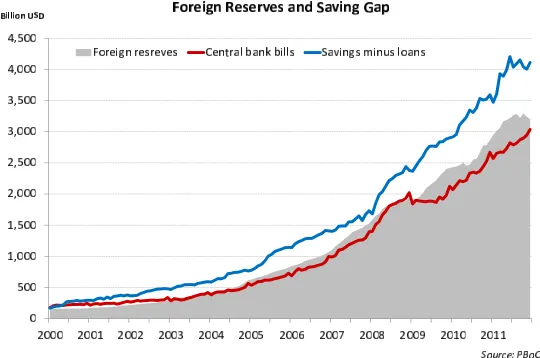
The gap between gross domestic savings and gross domestic loans signals some degrees

of credit frictions in these countries. The credit borrowing channel being constrained, the

need to save cannot be satisfied without the intervention of the public sector. We illustrate

this point using Chinese data (see Figure 4). As long as the wedge between domestic

savings and loans exists, the domestic financial market is repressed and the domestic real

interest rate is lower than the world interest rate. From here, we ponder whether there

exist some domestic structural deficiencies which caused domestic excess savings, leading

to a current account surplus and foreign reserve stockpiling.

(a) China

0

10

20

30

40

50

Pencentage point

1995 2000 2005 2010

year

reserves/GDP Private bond/GDP Public bond/GDP

(b) India

0

10

20

30

Pencentage point

1995 2000 2005 2010

year

reserves/GDP Private bond/GDP Public bond/GDP

(c) Indonesia

0

10

20

30

Pencentage point

1995 2000 2005 2010

year

reserves/GDP Private bond/GDP Public bond/GDP

(d) Philippines

0

10

20

30

40

Pencentage point

1995 2000 2005 2010

year

reserves/GDP Private bond/GDP Public bond/GDP

repression is Pareto sub-optimal for fast-growing emerging market economies with credit

constraints. As some domestic firms heavily rely on retained earnings for financing their

production, a repressed domestic interest rate would dampen firms’ retained earnings. 2)

Purchasing foreign reserve assets constitutes a second-best growth strategy in an economy

where the domestic financial market is under-developed (both for the lack of domestic

financial assets and for the existence of credit constraints) on the one hand and where

there are controls on capital flows.

It is worthwhile emphasizing the importance of capital controls to trigger foreign

reserve holding. In fact, capital controls constitute a way to discriminate public and

private capital flows, so that public capital outflows (i.e. purchasing foreign assets)

would not be entirely offset by private capital inflows (i.e. private external borrowing).

This imperfect substitutability can also appear by setting an ad-hoc external borrowing

constraint of domestic firms based on the asymmetric information facing international

investors (such as in Benigno and Fornaro (2012)). With this regard, China constitutes

an interesting illustration for my analysis, as in this country both financial market frictions

and capital controls are present. Therefore, in the subsequent sections, I will mainly focus

on the example of China.

Figure 4: Foreign reserves and gap between savings and loans in China

In the scope of this paper, I rule out the aspect of international trade and exchange

rate policies. This choice is explained by the need to focus on the relationship between

there is no consensus in academia on the (reverse) causality between foreign reserve

holding and exchange rate stability. We do not know whether keeping the domestic

currency undervalued is the objective of foreign reserve accumulation or both of them are

side effects of some other macroeconomic consideration.

1.2

A growth story of foreign reserve accumulation

Through which channel do foreign reserves affect economic growth? I argue that

the effect of foreign reserve accumulation goes through the fixed capital formation and

production efficiency gains.

Many academic works show that domestic capital accumulation remains the main

driver of economic catch-up in emerging economies - especially in East Asia - as the

neo-classical growth theory predicts. Based on this viewpoint, even the Chinese spectacular

growth rate is not a ‘miracle’; the contribution of fixed capital formation looms large (Yu

(1998), Nelson and Pack (1999), Song et al. (2011)).

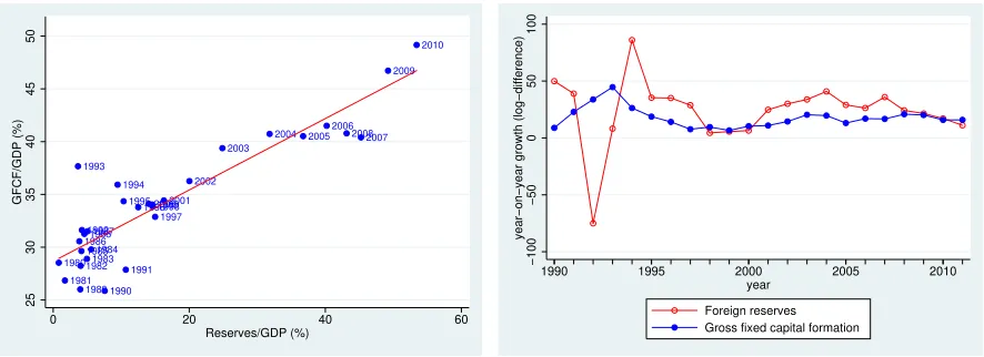
Figure 5 shows a clear positive relationship between foreign reserves to GDP ratio

and gross fixed capital formation to GDP ratio in China from 1980 to 2010. Figure 6

illustrates that the year-on-year growth rate of foreign reserves and that of gross fixed

capital formation coincide very closely since the mid-1990s in China. If we further test the

Granger causality of these two variables, we find that the growth rate of foreign reserves

leads that of gross fixed capital formation.

1980 1981 19821983 1984 1985 1986 1987 1988 1989 1990 1991 1992 1993 1994 1995 1996 1997 1998 1999 20002001 2002 2003 2004 2005 2006 2007 2008 2009 2010 25 30 35 40 45 50 GFCF/GDP (%)

0 20 40 60

Reserves/GDP (%)

Figure 5: Foreign reserves vs. GFCF (%GDP)

−100

−50

0

50

100

year−on−year growth (log−difference)

1990 1995 2000 2005 2010

year

Foreign reserves Gross fixed capital formation

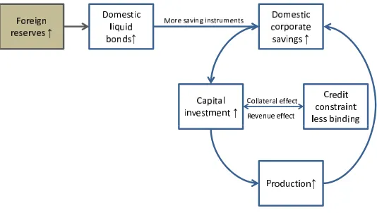
As illustrated in Figure 7, the story I tell in this paper is as follows: in a

financial-ly constrained economy, entrepreneurs need to make precautionary savings when they

harvest an output in order to overcome the credit constraint when they face investment

opportunities. In an fully open economy, this leads to a gap between domestic savings

and investment, thus current account surplus. However, if in addition there were capital

controls, entrepreneurs would not have direct access to international financial market in

order to make precautionary savings. In this case, the central bank can play the role

of financial intermediary and provide a domestic liquid bond with which domestic

en-trepreneurs can save. By issuing domestic liquid bonds, the central bank alleviates the

credit constraint facing investing entrepreneurs because firms can save more with the

pub-lic bond (volume increases) and domestic interest rate is less repressed (price increases).

As the domestic financial market is limited in its scope, the central bank can only invest

its bond proceeds abroad, in the form of foreign reserve assets. A further motivation for

the central bank to invest the bond proceeds abroad is that the world interest rate is

higher than the domestic interest rate as long as the domestic financial market is

con-strained and the domestic interest rate depressed. With the provision of domestic liquid

bonds, entrepreneurs will have higher retained earnings with which they can invest more

in capital regardless to the institutional credit constraint. Interestingly, capital plays a

dual role in this economy: it is not only the input for production, it is the collateral

for credit borrowing as well. With higher capital accumulation, the credit constraint is

further relaxed, all pushing the economy to achieve the first best level. There is indeed a

‘financial accelerator’ effect in the model.

As we can see in subsequent sections, foreign reserve accumulation constitutes a

second-best strategy during economic transition in the presence of credit and capital

account constraints. With this regard, the level of foreign reserves will increase until

the capital deepening is strong enough and/or the domestic private financial market is

Figure 7: Storyline

1.3

Review of the literature

This paper is related to two broad strands of literature: the motives of foreign reserve

accumulation, especially from a domestic structural viewpoint on the one hand and the

economic growth in the presence of credit constraints on the other hand.

A country may accumulate foreign reserves for reasons of different nature: to

consti-tute a buffer stock for the sake of crisis prevention or/and crisis management (

precau-tionary approach2_{,Bianchi et al.(2012)), to intervene in the foreign exchange market for}

the defense of a fixed exchange rate or for preventing the domestic currency from

appre-ciation (mercantilist approach3_{), or to hold foreign reserves due to domestic structural}

deficiencies (structural approach). My work is related in particular to the last approach.

According to this strand of literature, countries accumulate foreign assets as a

natural consequence of the wedge between domestic savings and investment. As

Gourinchas and Jeanne (2007) put it, ’the allocation puzzle is a saving puzzle.’

Accord-ing to this paper, the distortions in the domestic financial sector may induce domestic

precautionary savings. The distortions can be understood either in terms of the

capac-ity of a country to supply safe assets (Caballero et al. (2008)) or in terms of the credit

constraint facing domestic firms. In the presence domestic credit constraint, the

econo-my in its whole needs to make precautionary savings, generating a positive gap between

domestic savings and investment, source of capital outflows. Bacchetta and Benhima

2_{See Aizenman and Lee (2007),Aizenman and Hutchison (2010), Jeanne and Ranci`ere (2011),}

Benigno and Fornaro(2012)

(2010), Wen (2011) and Song et al. (2011) are the most relevant references with this

regard. Based on an open economy with a credit constraint facing firms which invest,

Bacchetta and Benhima (2010) show that the demand for foreign bonds is a complement

to domestic investment rather than a substitute. The reason behind is that foreign bonds

constitute supplementary corporate saving assets for credit-constrained firms. The

re-tained earnings can be used to invest in capital even if firms’ borrowing capacity can be

constrained. Therefore, in a fast growing economy, the demand for foreign bonds

increas-es with domincreas-estic capital formation. In the same vein, Song et al. (2011) shed light on

how a constrained access to bank loans of private firms compared to state-owned firms

can lead to a large level of corporate precautionary savings, thus to a persistent current

account surplus. As there is a gradual transformation of state-owned firms into private

ones, the overall precautionary savings increase, so do foreign reserves. Finally, Wen

(2011) tries to ‘make sense of China’s excessive foreign reserves’ by looking at household

savings. He argues that a large uninsured risk (e.g. the lack of a sound social safety net),

severe borrowing constraints, and rapid income growth can create an excessive level of

high household saving rates and large current account surpluses for emerging economies.

Therefore, foreign reserve accumulation is a natural consequence of a country’s fast

e-conomic catch-up with an inefficient financial system. As all the three papers look at

the demand for foreign assets in a small open economy setting with no capital controls,

the government/central bank is absent. The public and private capital flows are thus

perfect substitutes. What they examine is rather the change in a country’s net foreign

assets rather than the central bank’s foreign reserves per se. My current work differs from

theirs by targeting to the central bank’s reserve assets. Moreover, foreign reserves are

only a residual of private precautionary savings in these models while in my paper I argue

that the social planner may have an optimal policy to boost domestic capital investment

through purchasing foreign reserves.

In parallel, there is a strand of literature examining how policies of the

governmen-t/central bank help alleviate domestic credit constraint. A seminal paper by Woodford

capital investment in the presence of credit constraints. This paper is based on a financial

autarky setting.

One contribution of my current work is to combine the above-mentioned two

approach-es and the featurapproach-es of both a small open economy and a closed economy setting. To put it

in a different way, I examine the relationship between the demand for foreign assets and

domestic capital formation in an economy with capital controls; only the public sector,

e.g. the central bank, has a full access to international financial market. Private firms are

forbidden to borrow/lend abroad directly. The imperfect substitutability thus requires

the introduction of a central bank in the model. The model I present below will allow

us to examine whether accumulating foreign reserves constitutes an optimal policy for

the central bank. This paper is however not the first one which introduces a social

plan-ner (e.g. government or central bank) to discriminate public and private capital flows.

Bacchetta et al.(2012) and Benigno and Fornaro(2012) also examine the foreign reserve

accumulation in the presence of capital controls (Bacchetta et al.(2012)) or when private

flows are not perfectly substitutable to public flows based on their respective credibility

(Benigno and Fornaro (2012)).

My paper differs from Bacchetta et al. (2012) as I choose to use a production model

so that I can focus on the contribution of reserves to domestic capital formation,

driv-er of economic catch-up in emdriv-erging market economies. The introduction of capital is

very important for two reasons. First, by introducing domestic capital formation, I add

production efficiency gains when examining the optimal policy of foreign reserve

accumu-lation in the presence of credit constraint and capital controls, in addition to redistributive

effects and consumption smoothing gains. According to the literature of growth theory,

the gains from production efficiency have a much more persistent and stronger impact on

growth than that from pure consumption smoothing. This is thus a major contribution of

my paper compared to Bacchetta et al. (2012) who only focus on consumption

smooth-ing gains. Secondly, the introduction of capital formation makes my model settsmooth-ing more

relevant for countries with large stock of foreign reserves, such as China, as in my model,

My paper differs from Benigno and Fornaro (2012) as I model in a different manner

the imperfect substitutability between public and private capital flows on the one hand

and I consider a different motive of foreign reserve accumulation from their paper. While

Benigno and Fornaro(2012) study the precautionary and mercantilist motives of foreign

reserve accumulation, I focus on the imperfection of domestic financial market.

This paper is organized as follows. Section 2 describes the model setting. Section

3 analyzes the reserve accumulation and capital formation in a decentralized economy.

Section4introduces the optimal policy of the central bank. Section5presents a numerical

2

Model setting

Using a general equilibrium model with heterogeneous agents, the baseline model

economy is a small economy with a single consumption good. There are three types of

agents in the economy. Two symmetric entrepreneurs, a ‘hand-to-month’ labor and an

active central bank. We describe their behaviors as follows.

2.1

Entrepreneurs and their optimal behavior

Two symmetric infinitely lived entrepreneurs produce and consume in this economy

and they are occasionally constrained for credit borrowing every two periods when they

face productive investment opportunities. In fact, each entrepreneur changes status every

two periods, alternating between a ‘saving period (denoted S)’ and an ‘investing period

(denoted I)’, according to the following Markov chain.

   It+1 St+1   =M

   St It   =    0 1 1 0       St It   

Entrepreneurs’ budget constraints

A typical entrepreneur in his saving period receives the output from production

(cap-ital is chosen a period ahead) but does not have immediate productive investment plan

available and thus chooses to save part of the revenue for future investment. On the other

hand, in the investing period, an entrepreneur has immediate productive plans but does

not have sufficient funding to invest, therefore it needs to borrow to invest in physical

capital stock.

A typical entrepreneur who starts at timetwith a saving period will have the following

budget constraints every two periods.

At t :Πt−rtLt=cSt +St+1 (1)

That is, the saving entrepreneur uses his disposable income Πt to reimburse loans

subscribed a period ahead rtLt. It consumes cS

t and makes savings St+1 (in the form of

lending to the investing entrepreneur or of central bank bonds). In the next period, there

is a productive plan available, a saving entrepreneur becomes an investing entrepreneur

and uses his retained earnings to consume cI

t and to invest in capital stockKt+2. rt is the

domestic gross interest rate (rt >1, for all t). As the revenue during investing stage is

limited (no output available), the investing entrepreneur needs to make a loanLt+2 from

the other entrepreneur who is in his saving period (due to symmetry).

The other symmetric entrepreneur who starts at time t with an investing period will

have two reversed budget constraints as compared with above.

At t :rtSt+Lt+1 =cIt +Kt+1

At t+1 :Πt+1−rt+1Lt+1 =cSt+1 +St+2

Πt denotes the wealth of the entrepreneur at the beginning of his saving period t. It

comprises the production that the entrepreneur harvests using the capital stock invested

a period ahead and the labor hired at the current period, net of labor cost.

Πt =F(At, Kt, Nt)−wtNt (3)

At,Kt,Nt and wt denote respectively the labor-enhanced productivity, capital stock,

labor force and per capita wage.

The production function F(Kt, At, Nt) is a standard neoclassical production function:

increasing in all arguments, concave and homogeneous of degree one. We use FK,t and

FN,t to denote the marginal product of capital and of labor respectively.

Moreover, we introduce a passive fiscal policy (out of the hands of the central bank)

in the model by allowing distortionary taxes on capital and labor. Denote τK,t and τN,t

marginal rate of tax on capital and labor. Then we can express the after-tax marginal

˜

FK,t =FK,t−τK,t (4)

˜

FN,t =FN,t−τN,t (5)

Therefore, based on the chapter 15 of Ljungqvist and Sargent (2004), we can rewrite

the production function before and after tax payment in terms of the inputs and their

(after-tax) marginal products:

F(At, Kt, Nt) =FK,tKt+FN,tNt (6)

˜

F(At, Kt, Nt) = ˜FK,tKt+ ˜FN,tNt (7)

The advantage of doing so, as underlined by Ljungqvist and Sargent (2004), is that

we can treat ˜FK,t as a new variable independent from FK,t, similarly for ˜FN,t and FN,t.

Entrepreneurs’ program

Entrepreneurs maximize the intertemporal utility function:

∞

X

t=0

βt_U(cS

t) +βU(cIt+1)

(8)

As the two entrepreneurs are perfectly symmetric, we only need to look at the program

of the entrepreneur who starts with a saving period at time t.

Notice that one of the market failure of the model economy is that there is a credit

constraint facing the entrepreneur in his investing stage. This constraint is motivated

by the classic argument of the asymmetric information. Namely, as the lender (the

entrepreneur in his saving period) cannot guarantee the repayment of his debtor, he

requires a collateral when making loans.

This credit constraint in some emerging market economies are institutional in nature.

loans because of their status. The biggest Chinese banks are state-owned and prefer to

lend money to state-owned firms, as Song et al. (2011) details.

Following this argument, we model the credit constraint as below:

Lt+2 ≤

ψΠt+2

rt+2

(9)

The maximum loan that an investing entrepreneur can get is conditional on the

dis-counted value of the disposable income that the entrepreneur will obtain next period

when he harvest an output. ψ denotes the tightness of credit constraint, ψ ∈[0,1]. The

smaller is ψ, the tighter the constraint is.

To obtain the optimal behavior of an entrepreneur in a decentralized economy, we

maximize the equation (8) subject to (1), (2) and (9). And we obtain the following first

order conditions. Note thatλt+2u′(cSt+2) denotes the Lagrange multiplier associated with

the credit constraint at time t+ 2.

(1 +ψλt) ˜FK,t=rt(1 +λt) (10)

˜

FN,t =wt (11)

u′(cSt) = βrt+1u′(cIt+1) (12)

u′(cIt+1) =βrt+2u′(cSt+2)(1 +λt+2) (13)

Equation (10) tells us that the after-tax marginal product of capital is equal to the cost

of capital rt augmented by a coefficient 1+λt

1+ψλt, which is related to the credit constraint.

Equation (11) equalizes the after-tax marginal product of labor with unit wage. Equations

(12) and (13) are Euler equations. The Euler equation (13) which relates the marginal

utility of the consumption of an entrepreneur in investing state to that of the same

entrepreneur in saving stage depends clearly on the tightness of the credit constraint.

According to the Kuhn-Tucker conditions, the Lagrangian multiplier with respect to

λt+2u′(cSt+2)(rt+2Lt+2−ψΠt+2) = 0

Therefore, the credit constraint may be binding (rt+2Lt+2 = ψΠt+2) or non binding

(λt+2 = 0).

Notice that, when the credit constraint is binding, the investing entrepreneur at each

period cannot borrow as much as they would like to do, therefore they cannot absorb all

the funding the saving entrepreneur is willing to provide. This leads to a gap between

saving and loans in each period. The central bank can thus play a role in order to close

this gap. The strategy of the central bank is described later on.

2.2

Labor market

For simplicity, we assume that the labor supply is perfectly inelastic, namelyNtsupply=

1.

On the demand side, from the first order condition (11), we know that the marginal

product of labor, ˜FN,t, which is equal to wage w, is decreasing in labor demand Ndemand

t .

Therefore, we obtain a conventional decreasing labor demand function.

For a given level of technology At and capital stockKt, the labor demand and supply

functions uniquely pin down the wage and the equilibrium labor on the labor market.

Therefore, we are allowed to use this result from the labor market equilibrium

Ntsupply=Ntdemand= 1 henceforth.

Using this result and equation (11), we can rewrite the after-tax operational income

of family companies:

Πt = ˜FK,tKt+ ˜FL,tNt−wtNt (14)

= ˜FK,tKt (15)

Note that as the labor is inelastic in the model, the marginal tax on labor does not

lump-sum tax (transfer) to the labor force which is out of our scrutiny.

2.3

The central bank’s Behavior

The hallmark of this paper is that we explicitly model the behavior of the central bank

in the model economy. We argue that the central bank can provide a liquid central bank

bond, which is used as a supplementary saving instrument for the saving entrepreneur.

As we will show later on, this may be a second-best strategy of the central bank when

the domestic financial market is under-developed.

General setting

Several characteristics about the central bank in our model needs to be underlined.

First of all, the central bank is a consortium of the monetary authority and the commercial

banks. This setting is plausible as in China the banking system is mainly state-owned.

In fact, according toWalter and Howie (2012), more than 90 percent of total commercial

banking assets is state-controlled in China.

Secondly, the central bank is the only player which has access to international financial

market in our model economy. This situation is dubbed by Bacchetta et al. (2012) as

a ‘semi-open’ economy. This way of modeling corresponds to what we observe about

China’s capital account management. In fact, China not only accumulates foreign reserves

but also closely control capital inflows and outflows. The private sector does not have

a full access to the international financial market. Within the scope of the paper, we

assume that the capital controls which make domestic private capital flows and public

capital flows imperfectly substitutable are institutional in nature and cannot be removed

in the short-run. To our understanding, the need of setting capital controls are closely

related to the under-development of the domestic financial market which is the focus of

our analysis.

Thirdly, the central bank does not control fiscal policy which is in the hands of the

government. As the State is the ultimate shareholder of the central bank, we argue

intertemporal budget constraint.

Finally, the central bank is forbidden to finance the government debt by law. Namely,

the central bank cannot purchase any government bonds.

The central bank’s flow budget constraint is described as follows:

rt∗Bt∗+Bt+1+Tt

| {z }

resources

=rtBt+Bt∗+1+ Φ

2 B

∗

t+1−Bt∗

2

| {z }

expenses

(16)

, where Tt=τK,tKt+τN,t

The central bank receives tax revenue Tt from entrepreneurs as well as returns on

foreign reserve holdings r∗

tBt∗ from abroad and domestic liquid bond proceeds Bt+1. On

the side of expenses, the central bank needs to pay back the liquid bond issued a period

ahead rtBt and to decide the amount of foreign reserves to purchase B∗

t+1. Notice that

accumulating foreign reserves is not costless. A quadratic adjustment cost B∗

t+1−B∗t

2

is introduced to take into account the costs of foreign reserve holding and to

preven-t explosive solupreven-tion in small open economy model (following Schmitt-Grohe and Uribe

(2003)). We further assume that the central bank does not consume.

Interaction between the private sector and the central bank

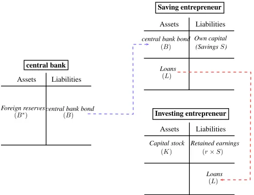
What is the role played by the central bank in our model economy. We present below

the balance sheets of the central bank and of the private sector for illustration.

In fact, by providing a liquid central bank bond, the saving entrepreneur can save up

to first-best level with this supplementary saving instrument. Therefore the retained

earn-ings of this entrepreneur in the investing period will increase, allowing the entrepreneur

to invest more in capital stock.

The central bank’s choice of purchasing foreign reserve assets

The use of public debt, e.g. government or central bank bonds, has proved to be

a welfare-improving strategy to raise domestic capital formation, as Woodford (1990)

central bank bond Foreign reserves

Assets Liabilities

(B) (B∗₎

Own capital

Assets Liabilities

(SavingsS) central bank bond

(B)

Loans

(L)

Retained earnings

Assets Liabilities

(r×S)

Capital stock

(K)

Loans

(L)

Saving entrepreneur

Investing entrepreneur central bank

Figure 8: Balance sheet of the central bank and the private sector

the central bank needs to invest the bond proceeds abroad. There are not available

alternatives. As a result, massive foreign reserve accumulation is a natural consequence

of a growth strategy aiming at promoting domestic capital formation.

Based on the experience of China, several arguments can be advanced to explain why

the central bank has to invest bond proceeds in foreign assets. First, the domestic financial

market is very shallow in scope; as a result the domestic investment opportunities are

limited. According to Walter and Howie (2012), in China ‘the banks are the financial

system’ and ‘it is bank lending and [public] bond issuance that keep the engine of Chinas

state-owned economy revving at high speed.’ Besides the bank deposits and loans (which

are integrated into the private sector in our model), the private bond market and equity

markets are very small. For example, in 2007 which was a record year for Chinese equity

financing, more than 123 billion of U.S. dollar was raised on the equity market, but in the

same year, banks extended new loans totaling 530 billion of dollars and total debt issues

in the bond market accounted for another 355 billion. Now, if we look at more carefully at

the Chinese bond market, we observe that this market is dominated by public obligations,

i.e. government debt, central bank bond and policy bank bond issuance. Corporate and

commercial papers are very recent financial products and their weight on domestic bond

market is negligible (around 5%) compared to the public issuance (Figure 9).

Figure 9: Public bonds vs. private bonds

by the Law of the People’s Bank of China of 1995 and its amendment in 2003. The

proportion of the central bank bonds has steadily increased from 2002 to 2010, a period

when Chinese foreign reserves have rapidly increased and the government’s capacity of

issuing new debts was limited.

Figure 10: Decomposition of the Chinese bond market

Finally, the domestic financial system is mainly state-owned. If the central bank

The central bank’s policy

In order to promote domestic economic growth, the central bank has mainly three

instruments: domestic interest rate, liquid bond issuance and foreign reserve purchasing,

as indicated in the table below.

Table 1: Different variables

Central Bank policy Market variables Exogenous fiscal policy

rt+1 cSt, cIt τK,t, τN,t

Bt Kt+1

B∗

t St+1,Lt+1

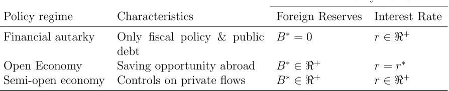
The usefulness of the instruments depends on the policy regime that a country has.

We will below compare several policy regimes in order to see whether accumulating foreign

reserves consists of an optimal policy for the central bank. Different policy regimes are

defined as follows, according to Bacchetta et al. (2012).

Table 2: Policy regimes

Policy Instruments

Policy regime Characteristics Foreign Reserves Interest Rate

Financial autarky Only fiscal policy & public

debt

B∗ _{= 0 r∈ ℜ}+

Open Economy Saving opportunity abroad B∗ _{∈ ℜ}+ _r=r∗

Semi-open economy Controls on private flows B∗ _{∈ ℜ}+ _{r∈ ℜ}+

Notice that in this model, the financial intermediary is absent in this model. However,

the results that I derive in the subsequent sections will not change if a perfectly

competi-tive banking sector is introduced. Therefore, to keep the model tractable, I decide to put

2.4

Market clearing

On the financial market

The amount of the liquid bonds that the central bank provides is equal to the difference

between the savings of the saving entrepreneur and the loans asked by the investing

entrepreneur at each period, namely,

Bt

|{z}

supply of liquid bonds

= St−Lt

| {z }

demand for liquid bonds

(17)

A positive Bt is motivated by the fact that the investing entrepreneur is financially

constrained. Otherwise, the borrowing need Ltoughts to absorb all the savings St on the

financial market, leading to Bt= 0.

On the good market

Output produced by the saving entrepreneur is consumed by both entrepreneurs and

the labor force, to invest in capital investment or to buy foreign reserves. We thus have

the following aggregate clearing condition:

F(At, Kt) = cS t +c

I

t+wt+Kt+1−(r∗t−1)Bt∗+ Bt∗+1 −Bt∗

| {z }

current account balance

+Φ

2 B

∗

t+1−Bt∗

3

Market equilibrium without public intervention

In this section, I present some fundamental characteristics of the model which can

be analytically derived in a decentralized market equilibrium. I can show the saving

entrepreneur tends to make precautionary savings, knowing that he will be constrained

for borrowing next period in his investment stage. Moreover, I demonstrate that when the

financial constraint is strong enough (ψ < 1₂), in steady state, the constraint is binding

and the constrained steady state is uniquely determined. Finally, I will show how the

central bank policy can ameliorate the capital formation in the model economy. In

order to derive analytical results, I use log-utility and Cobb-Douglas production function

henceforth, namely U(ci

t) =log(cit), i∈(S, I) and F(Kt, At) =KtαA1t−α.

Definition 1 A perfect foresight market equilibrium in a decentralized economy is a

se-quence of prices {wt, rt} and an allocation {cS

t, cIt, Kt+1, St+1, Lt+1}, for a given policy

set{B∗

t, Bt, τK,t, τN,t}(t= 0,1,2, ...), and for given initial conditions{K0, L0, S0, B0, B0∗},

such that for all t≥0:

1. Given prices and the government policy, {cS

t, cIt, Kt+1, St+1, Lt+1} satisfy the first

order conditions (10) to (13)

2. Government budget constraint is verified (16)

3. Financial and good markets are cleared: (17) and (18)

Notice that depending on the economic policy regime, the central bank can use all or

part of its policy instruments {rt, Bt∗, Bt}.

With the log-utility and equations (1), (2),(12), (13), we can show that the optimal

consumption derived from each entrepreneur’s utility maximization program represents

a constant share of the entrepreneur’s initial wealth at the beginning of the period (See

cS

t = (1−β)(Πt−rtLt) (19)

cIt = (1−β)rtSt (20)

Then, we obtain:

St+1 =β(Πt−rtLt) (21)

Kt+2−Lt+2 =βrt+1St+1 (22)

3.1

Entrepreneurs’ precautionary savings

We can first show a common result as the literature of domestic financial

under-development is used to present: due to the credit constraint entrepreneurs save more

than in a perfect market without credit frictions. This extra savings correspond to the

‘precautionary savings’ of the saving entrepreneur who anticipates the credit constraint

that he will face a period later when there will be a productive investment plan.

Indeed, when the credit constraint is binding, the savings made by the saving

en-trepreneur is determined using (1), (2) and the optimal intertemporal allocation from the

saving stage to the investing stage 12:

St+1 = 1

1 +β

 

β(1−ψ) ˜FK,tKt | {z }

predetermined

+Kt+2

rt+1

−Lt+2

rt+1

 

 (23)

As the credit constraint is binding, Lt+2 ≤ L∗t+2, L∗t+2 being the level of borrowing

when the credit constraint is absent. Therefore, St+1 ≥ St∗+1, St∗+1 being the private

savings in the absence of any credit constraint. The saving entrepreneur saves thus more

3.2

Capital formation

How does the capital stock evolve over time? From (22), the capital accumulation

consistent with optimal consumptions satisfies:

Kt+2 = βrt+1St+1

| {z }

retained earnings

+Lt+2

|{z}

loans

(24)

=β2rt+1(1−ψ) ˜FK,tKt+ψFK,t˜ +2Kt+2

rt+2

(25)

Notice that the retained earnings and the loans are reversely affected by interest

rates. An increase in domestic interest rate raises the retained earnings of the saving

entrepreneur (revenue effect) but reduces the loans that the investing entrepreneur may

make (price effect). Therefore, for any entrepreneur, the stock of capital is affected by

two-period interest rates. Whether the capital stock increases or decreases depends on

which effect dominates.

We also observe a financial accelerator effect in equation (25). An initial positive

shock on the retained earnings (either an increase in rt+1 or an increase in initial capital

stock ˜FK,tKt) will lead to an increase in capital formation at tt+2, which in turn drives

up loans. As a result, contemporary capital formation further increases, generating a

virtuous cycle.

From (25), one can easily show that ceteris paribus

∂Kt+2

∂rt+1

>0

∂Kt+2

∂rt+2

<0

3.3

Steady state

I now study the steady state of the decentralized economy. I normalize all policy

variables by the disposable income Π = ˜FKK. Namely we define b∗ ₌ B∗

Π, b =

B

Π and

˜

τ = T

From the central bank’s budget constraint (16), we know that

(r∗−1)b∗+ ˜τ = (r−1)b (26)

Given international and domestic interest rates, we observe from the equation above

that if the central bank wants to provide liquid assets in the domestic economy, it can

achieve this objective either by raising distortionary taxes or by purchasing foreign

re-serves. The foreign reserve purchasing allows the central bank to provide liquid assets

without distorting the economy.

Uniqueness of the binding steady state

Now, we show that the steady state is uniquely determined.

From (12) and (13), we know that in steady state

• the credit constraint is binding when r < _β1 (βr)2 ₌ 1

1+λ <1

• the credit constraint is unbinding when r = _β1

Proposition 1 The financially constrained steady state is uniquely determined if 0 ≤

b < β(1−2ψ).

Proof. See Appendix B

From Proposition 1, we can conclude that the credit constraint is not binding when

b ≥ β(1−2ψ); the central bank can achieve this goal by raising b∗ _{or ˜τ. The credit}

constraint is binding when 0 < b < β(1−2ψ). We also observe that with the credit

constraint, the domestic interest rate is repressed and lower than the world interest rate

1

β. When the central bank provides liquid bonds which were scarce in the economy, it

lowers the price of the liquid bonds and pushes the domestic interest rate up to the world

interest rate level. r is indeed increasing in b: r = _β(1−ψ_ψ)−b

We can further prove that the coefficient of the tightness of the credit constraint is

important for whether the credit constraint is binding in the steady state. When ψ ≥ 1₂,

the credit constraint is unbinding in the steady state. Whenψ < 1₂, the credit constraint

We can further look at the different steady states in different policy regimes described

in Table 2.

Financial autarky In a closed economy whereB∗ _{= 0, ifψ ≥1/2, the credit constraint}

does not bind in the steady state. In this case,βr= 1, namely, the domestic interest rate

is equal to the world interest rate (assuming the same time preference). K =A(αβ)1−1α,

capital stock achieves its first-best level, assuming that there is no distortionary tax

τK = 0. And the consumptions are perfectly smoothed, namely the consumptions in the

saving stage and the investing stage are equalized cI _=cS_.

If ψ < 1/2, the credit constraint binds in the steady state. The Lagrange multiplier

associated with the credit constraint is thus positive, λ = 1

β2_r2 −1 > 0. We have the

domestic interest rate less than the world interest rate, namely βr = ₁₋ψ_ψ < 1. Capital

stock cannot achieve the first-best level, K = Ahα (1−ψ)β2_{r +} ψ

r

i1−1α

. As for the

consumptions, that of the investing stage is always smaller than that of the saving stage,

cI

cS =

ψ

1−ψ <1.

In fact, in a financial autarky, with the productivity growth, the more capital the

bet-ter. There is thus a strong demand for liquid assets. However, investors are constrained

and the central bank does not have sufficient resources to provide domestic assets

with-out distorting the domestic economy. Therefore, the economy may be constrained if the

credit constraint is very tight.

Open economy One big difference compared to the financial autarky is that the

domes-tic interest rate is always equal to the world interest rate in the steady state, r=r∗ ₌ 1

β.

In this case the credit constraint in never binding, leading to b = b∗ _{= β(1−2ψ), in}

the absence of distortionary taxes. In an open economy, both the central bank and th

saving entrepreneur have access to international financial market, therefore, the saving

entrepreneur can make deposits abroad. In aggregate, there are sufficient foreign assets

to increase saving revenues of domestic entrepreneurs. Therefore, in steady state, the

Table 3: Decentralized economy

Economic Structure Steady State ψ

Financial autarky constrained ψ < 1

2

unconstrained ψ ≥ 1₂

Open Economy unconstrained ∀ψ

The capital formation in the steady state

In the steady state, how the capital stock evolves over time with policy variables?

Previously we demonstrate that the capital stock is composed of retained earnings and

borrowing and that retained earnings are increasing in the interest rate while borrowing

is decreasing in the interest rate. The capital stock thus depends on both the revenue

effect and of the price effect of interest rates.

Proposition 2 The capital stock represents a U-shape curve as a function of βr.

Pur-chasing foreign reserves, which leads to a higher supply of domestic liquid assets and thus

a higher interest rate, helps increase the capital stock and raise the production in the

economy.

Proof. See Appendix D

For simplicity, we ignore distortionary taxes which will only shift the U-shape curve

in Figure 11vertically but do not change the shape of the curve.

From Figure11, we observe that the capital stock achieves its first-best level ifβr= 1

(i.e. when the credit constraint is not binding) or if βr = ₁₋ψ_ψ. In the first case where

βr = 1, the economy is in the steady state with an unconstrained credit constraint (i.e.

either in a full open economy or in a financial autarky with ψ ≥ 1

2). In the second case

where βr = ₁₋ψ_ψ, the economy is in a financially autarkic steady state where the central

bank does not provide any liquidy saving instruments.

When ₁₋ψ_ψ ≤ βr ≤ q₁₋ψ_ψ, the curve is decreasing. when the central bank starts

to provide liquid bonds, this raises the interest rate, leading to a more stringent credit

constraint and thus a lower level of borrowing. At the same time, as the financial market

βr

K A

1−α

1 ψ

1−ψ

q ψ

1−ψ αβ

Unconstrained Steady State Constrained Steady State w/o Liquid Bonds

Figure 11: U-shape capital stock

sufficient saving instruments on the market. Therefore, on this part of the curve, the

price effect of the interest rate dominates the revenue effect, leading to a decrease in the

capital stock.

When q₁₋ψ_ψ ≤βr≤1, the curve is increasing. This is because when the central bank

provides more and more liquid assets, the price of these assets further decrease and raise

even more the interest rate, any entrepreneur in his saving stage can save up to the

first-best level and the retained earnings increase with the interest rate. Bear in mind that the

retained earnings are used for capital investment a period later when the entrepreneur

faces investment opportunities. The revenue effect dominates the price effect on this part

of the curve.

We can gain a more precise insight of how capital formation evolves with the interest

rate by examining the following equation (derived in Appendix D):

˜

FK = r

(βr)2_{+ψ[1−(βr)}2_] (27)

We identify three effects which affect the capital stock in the economy:

• Opportunity cost of capital,r

• Revenue effect, (βr)2 ₌ 1

1+λ

The first effect, opportunity cost of capital, is standard: the higher is r, the higher

is the cost of investing in capital stock compare to buying bonds, the less capital is

demanded. The other two effects are particular in our model.

The second term (βr)2 _{is related to the credit constraint in the economy. As}

en-trepreneurs are occasionally credit-constrained, they have incentives to partly rely on

retained earnings (precautionary savings) in order to be able to invest in capital even

they are constrained. As the retained earnings are increasing in interest rate, this

ef-fect has a positive impact on capital stock (i.e. revenue efef-fect). Notice that the square

appears as the capital is invested every two periods. In an extreme case, when ψ = 0

(the constraint extremely binding), the second effect clearly dominates the first one. As

a result, a higher supply of the liquid bonds leads to a higher domestic interest rate,

unambiguously increasing the capital stock.

The third effect stems from the fact that the loans that an investing entrepreneur can

make is conditional on the discounted valued of the future production. An increase in r

decreases the borrowing capacity of investing entrepreneurs, as it lowers the discounted

value of the collateral. The interest rate has thus a negative price effect on capital

stock. As described above, the price effect dominates the revenue effect when the supply

of liquidity is very low, as in this case the collateral value of capital becomes so large

that it dominates the other effects. However, the capital formation has a feedback loop

effect on the credit constraint. Namely, more capital invested provides stronger collateral

in the next period, allowing investing entrepreneurs to borrow more money during the

investing stage and leading to a looser credit constraint. As the credit constraint becomes

less stringent, this third effect becomes less important and is dominated by the revenue

effect. The tightness of the credit constraint can also dampen the collateral effect on

capital, making the revenue effect stronger than the price effect.

As long as the central bank provides liquid bonds B by purchasing foreign reserves

B∗_{, it can push up domestic interest rate to the world interest rate and to push domestic}

4

The central bank’s optimal policy

Until now we have analyzed the fundamental characteristics of our model and its

steady states, both when the credit constraint is binding or unbinding. We have also

examined two policy regimes - financial autarky and open economy. In the first case,

the central bank, along with a latent government setting tax rates, uses public bond and

interest rate to adjust the economy. In the second case, when the economy is fully open,

the private sector has a direct access to international financial market to eliminate the

domestic credit constraint. As a result, the central bank is somewhat bypassed by the

private sector.

Now we examine the central bank’s policy in a semi-open economy, namely when the

central bank is the only one which can borrow or lend abroad. In such a policy setting,

can the public intervention of the central bank improve the welfare of the economy? We

use here the Ramsey problem presented in Chapter 15 ofLjungqvist and Sargent(2004).

4.1

General setting

We assume that the central bank optimizes the consumptions of contemporaneous

en-trepreneurs in their different stages as well as the labor income, according to the following

objective function. Remember that in a semi-open economy, the central bank can decide

both the amount of foreign assets to purchase, B∗

t+1, and the domestic interest rate rt+1.

max

{St+1,Lt+1,Bt∗+1,Kt+1,cSt,cIt,wt,rt+1,λt+1}

∞

X

t=0

βt

(

u(cSt) +u(c I

t) +ωu(wt)

)

(28)

Definition 2 (Ramsey problem) The central bank’s optimal policy consists of

choos-ing a sequence of policy variables {Bt∗+1, Bt+1, rt+1}∞0 such that:

• The corresponding competitive equilibrium allocation (10) to (13) maximizes the

welfare function (28)

• Individual entrepreneurs’ budget constraints, (1) and (2), are verified

• Bond market (17) is cleared

The way to solve the Ramsey problem follows the “Primal Approach” described by

Erosa and Gervais(2001).

The full Ramsey problem is presented below. Equation (11) is used to substitute ˜FN,t

by wt.

max

{St+1,Lt+1,B∗t+1,Kt+1,cSt,cIt,wt,rt+1,λt+1}

∞

X

t=0

βt

(

u(cSt) +u(c I

t) +ωu(wt)

+ηtS

h

˜

FK,tKt−rtLt−cSt −St+1

i

+ηI t

rtSt+Lt+1−cIt −Kt+1

+ηtG

FK,tKt+FN,t−cSt −c I

t −wt−Kt+1−Bt∗+1+rt∗Bt∗−

Φ

2 B

∗

t+1 −Bt∗

2

+θSt

1

cS t

−βrt+1 1

cI t+1

+θIt

1

cI t

−βrt+1(1 +λt+1) 1

cS t+1

+ρth(1 +ψλt) ˜FK,t−rt(1 +λt)i

+Λt

h

ψFK,tKt˜ −rtLti

)

F OC(St+1) :ηS

t =βrt+1ηIt+1 (29)

F OC(Lt+1) :ηtI =βrt+1 ηtS+1+ Λt+1

(30)

F OC(B_t∗₊₁) :ηG t

h

1 + Φ(B∗_t+1−B_t∗)i =βr_t∗₊₁ηG t+1

h

1 + Φ(B

∗

t+2−Bt∗+1)

r∗

t+1

i

(31)

F OC(Kt+1) :βηtS+1FK,t˜ +1−ηIt −η G t +βη

G

t+1FK,t+1+βψΛt+1FK,t˜ +1 = 0 (32)

F OC(cS t) :

1

cS t

−ηS t −η

G t −

θS t

(cS t)2

+ θ

I

t−1rt(1 +λt) (cS

t)2

= 0 (33)

F OC(cIt) :

1

cI t

−ηIt −η G t −

θI t

(cI t)2

+ θ

S t−1rt (cI

t)2

= 0 (34)

F OC(rt+1) :βηtI+1St+1−β ηSt+1+ Λt+1

Lt+1−β

θS t cI

t+1

−βθI t

(1 +λt+1)

cS t+1

−βρt+1(1 +λt+1) = 0

(35)

F OC(λt+1) : −θ

I tβrt+1 cS

t+1

+βρt+1

ψFk,t˜ +1−rt+1

= 0 (36)

We can also derive the first order conditions with respect to ˜FK,t+1 or/and ˜FN,t+1(wt),

if we allow the central bank to set tax rates as well.

F OC( ˜FK,t) :ηS

t+1Kt+1+ρt+1ψλt+1+ Λt+1ψKt+1 (37)

F OC(wt) : ω

wt −η G

t = 0 (38)

4.2

Steady state

When the central bank actively uses its policy instruments{Bt+1, Bt∗+1, rr+1}to adjust

the economy, what is the steady state it can achieve?

Financial autarky

In the financial autarky, the first order condition (31) is no longer relevant, B∗ _{= 0.}

Whether the steady state is financially constrained depends thus on, as in the

Proposition 3 The central bank can achieve the steady state with an unconstrained credit

constraint when the coefficient of the tightness of the credit constraint ψ ≥ 1₂. That is,

λ= Λ = 0, βr= 1 and cS _=cI_{. When ψ <} 1

2, the steady state with the Ramsey policy is

constrained. That is, λ >0, Λ >0, βr <1 and cI _{< c}S_.

Open economy

Proposition 4 The central bank can achieve the steady state with an unconstrained credit

constraint in an open economy by using an optimal policy `a la Ramsey. That is, the

central bank can achieve the same steady state as the decentralized economy does in an

open economy.

Proof. See Appendix E

4.3

Economic transition in a semi-open economy

We have seen so far that the steady state does not change in the Ramsey program

compare to the decentralized economy, both in a financial autarkic setting or in an open

economy. How about the economic transition in a semi-open economy towards a steady

state where the economy will be fully open? In a semi-open economy, the central bank

has two instruments in its hands: central bank bond and interest rate. Therefore, we

argue that the Ramsey program in a semi-open economy is welfare improving compare

to a financial autarky or an open economy.

Indeed, the foreign reserve accumulation is a second-best strategy of economic growth,

taking into account both credit constraint and capital controls. A combined use of capital

controls and foreign reserve holding allows the central bank to have sufficient funding to

provide liquid assets within the country and at the same time to be able to adjust domestic

interest rate whenever it is necessary.

F OC(rt+1) : ηI

t+1St+1− ηSt+1+ Λt+1

Lt+1

| {z }

redistributive effects − θ S t cI t+1 − θ I

t (1 +λt+1) cS

t+1

| {z }

intertemporal choices

−ρt+1(1 +λt+1)

| {z }

opportunity cost = 0

When the capital account is closed and the central bank accumulates foreign reserves,

it can control domestic interest rates subject to different policy objectives. When the

central bank increases domestic interest rate, this is beneficial for the investor of the

next period as the revenue from savings will be higher (first term). However, this will

be harmful for the saver of the next period as it has to pay higher interests of loans

they made during the investment stage (second term). It will also change intertemporal

behavior of entrepreneurs, leading to more savings and less consumption, thus decreasing

social welfare (third and fourth terms). Finally, a higher domestic interest rate implies

higher opportunity cost, therefore the capital investment will decrease (the last term).

The first two terms translate a redistributive trade-off that the central bank has to face.

This redistributive effects also imply welfare costs to the economy. Indeed, if the current

investors are very constrained and the central bank thinks the long run steady state can

be achieved soon, it has incentives to decrease the interest rate to alleviate the interest

burden of investing firms. If on the contrary the central bank believes that the economy

will still be constrained for a long period, it has incentives to rise domestic interest rate,

so that the current savers may transfer a larger amount of interest revenue to the future

when they will be constrained.

Depending on the tightness of the credit constraint and the speed of convergence to

the steady state, the central bank can decide to favor savers or investors in order to

enhance the social welfare.

Denote Ht the left hand side of the equation (35). We can show that

Ht =

∞

X

i=1 Λt+2i

!

St+1−

∞

X

i=1

Λt+2i+1

!

In sum, when Ht is different from 0, the central bank has incentives to intervene and

the open economy does not provide an optimal equilibrium. If Ht >0, the central bank

has incentives to raise interest rate to favor savers. If Ht < 0, the central bank has

incentives to lower interest rate. In general, as Table 4 shows, with financial frictions

an open economy is suboptimal during transition while an economy with closed capital

account and sufficient foreign reserves can achieve higher social welfare during transition.

Table 4: Static vs. Dynamic approach

Central Bank Intervention

Economic Structure Steady state Dynamics

Financial autarky depending onψ suboptimal

Open Economy unconstrained suboptimal

Semi-open unconstrained optimal

5

Numerical study

5.1

Calibration

We simulate our model in a semi-open economy using Dynare 4.3.2 (see

Adjemian et al. (2011)). The shock comes from an unanticipated productivity growth

which is exogenous to the model. From this exercise, we will see how during a fast

grow-ing economic transition, the foreign reserve accumulation, combined with a closed capital

account, helps the model economy to achieve the first-best level of capital stock.

The shock on At follows the process below:

At = (1 +gt)At−1 (40)

gt=σgt−1+ǫt (41)

The accelerator of the growth rate, σt, is less than 1, ensuring the growth rate

con-verges to 0. The growth rate gt can be disturbed by an exogenous shock denoted ǫt. We

assume that ǫt is a white noise and we denote g0 the initial technology growth rate.

I calibrate the model based on the recent literature on economic growth and foreign

reserve accumulation in an economy with financial constraints. Song et al. (2011) is an

important reference as it is the most recent theoretical paper on the strategy of economic

growth in China in the presence of financial constraint. However, I need to point out

that I do not pretend to quantitatively explain the foreign reserve accumulation in China

since the early 2000s due to the simplicity of the model. I aim at illustrating with my

numerical results a qualitative analysis of the foreign reserve policy in an economy with

Table 5: Calibration

Symbol Meaning Value Remarks

α share of capital in the production 0.33

β discount fact 0.95

ψ credit constraint tightness 0.1 keeping the constraint binding

g0 initial growth rate 0.10 targeting an annual growth rate

of 10%

σ technology growth rate

autocor-relation coefficient

0.6 generating a lasting growth path

ω share of the labor income in the

Ramsey objective function

1

φ adjustment cost of purchasing

re-serves

0.01

5.2

The demand for foreign assets as a response to the credit

constraint

First of all, my model can replicate the results that the existing literature has

illustrat-ed about the foreign reserve accumulation in the presence of domestic crillustrat-edit constraints

(in a fully open economy): the more stringent is the credit constraint, the higher domestic

savings are, leading to a current account surplus and foreign reserve stockpiling.

The blue line in Figure12and13represents the situation whereψ = 0.05 (tight credit

constraint) while the black line represents the opposite situation where ψ = 0.45 (loose

credit constraint). Notice that a tighter credit constraint encourages entrepreneurs to

save more, for that the central bank has to provide a larger level of domestic liquid bond.

Due to the constrained domestic financial market, the provision of central bank bonds

requires more investment in foreign reserves. It is interesting to see that in case where

the credit constraint hardly binds (the black line), the demand for domestic central bank

bond and for foreign assets is very low.

In terms of welfare, we observe that entrepreneurs are better off regardless to their

stage, as the supply of central bank bond increases entrepreneurs’ retained earnings and

lowers their debt burden. As for capital accumulation, there is a gap, during

transi-tion only, between the levels of capital stock when the credit constraint is very binding

constrained domestic financial market allows the capital accumulation to achieve the

unbinding steady state slightly faster than when the constraint is more binding.

0 5 10 15 20 0.55

0.6 0.65 0.7 0.75

Output

0 5 10 15 20 0.16

0.18 0.2 0.22 0.24

Capital formation

0 5 10 15 20 4

6 8 10 12x 10

−3 _{Consumption of savers}

0 5 10 15 20 4

6 8 10 12x 10

−3 _{Consumption of investors}

0 5 10 15 20 0.35

0.4 0.45 0.5

simulation period Consumption of the labor

0 5 10 15 20 0

1 2 3

simulation period Gross interest rate

ψ = 0.05 ψ = 0.15 ψ = 0.25 ψ = 0.45

0 5 10 15 20 0.05

0.1 0.15 0.2 0.25

Savings

0 5 10 15 20 0

0.05 0.1 0.15 0.2

Loans

0 5 10 15 20 0

0.1 0.2 0.3 0.4

Domestic bond

0 5 10 15 20 0

0.1 0.2 0.3 0.4

Foreign assets

0 5 10 15 20 −0.02

−0.01 0 0.01 0.02

simulation period Current Account

0 5 10 15 20 0

0.05 0.1 0.15 0.2

simulation period Constraint

ψ = 0.05 ψ = 0.15 ψ = 0.25 ψ = 0.45

5.3

Economic transition in a semi-open economy

We can see from Figure 14that the central bank’s optimal policy in an economy with

capital controls allows a fast transition than in an open economy. By accumulating more

foreign reserves during transition (B∗_{), the central bank is able to issue more domestic}

liquid assets (B) and with capital controls it raises domestic interest rate (r). This leads

to higher domestic corporate savings (S) and thus higher capital investment (K). The

revenue effect of the interest rate overrides the price effect as we observe that the loans

asked by the investing entrepreneur decreases as the domestic interest rate increases.

Domestic consumption levels are also higher for both types of entrepreneurs. Notice

that the accumulation of foreign reserves will stabilize when the financial deepening (the

capital-to-output ratio) is sufficiently large.

If we look at Chinese data, we can observe that along with massive foreign reserve

accumulation in China the supply of the central bank’s assets (e.g. central bank bonds

or required reserves) has increased massively (see Figure 4). The surge in the central

bank’s assets has absorbed the liquidity in private sector and has forced entrepreneurs to

save instead of consuming more. In this way, capital is channeled to productive plans,