Simulation Based Design Analysis of an Adjustable Window Function

ISSN Online: 2159-4481 ISSN Print: 2159-4465

Simulation Based Design Analysis of an Adjustable

Window Function

Orvila Sarker

_{, Rezaul Huque Khan}

1_{Department of Information & Communication Technology, Comilla University, Comilla, Bangladesh}

2_{Department of Applied Physics, Electronics & Communication Engineering, University of Chittagong, Chittagong, Bangladesh}

Abstract

Window based Finite Impulse Response filters have the problem that in order to ob-tain better performance from these filters in terms of minimum stopband attenua-tion cost has to be paid for half main-lobe width and vice-versa. A soluattenua-tion of this contradictory behavior is to increase the length of the window which in turn requires more hardware hence increasing the cost of system. This paper proposes a novel window based on two shifted hyperbolic tangent functions. The proposed window contains an adjustable parameter, with the help of which desired time and frequency domain characteristics may be achieved for relatively shorter window length. The characteristics of the proposed window are compared with those of the two well-known adjustable windows namely Cosh window and Exponential window. MATLAB simulation results show that for the same value of window length, the proposed window provides improved output, and thus it makes a good compromise between minimum stopband attenuation and half main-lobe width compared to the windows mentioned previously.

Keywords

Finite Impulse Response Filter, Minimum Stopband Attenuation, Half Main-Lobe Width

1. Introduction

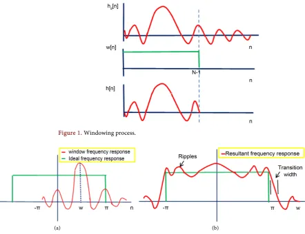
Ideal filters have perfectly flat passband with infinite attenuation in the stopband. Un-fortunately these filters are practically unrealizable because of their infinite number of co-efficients in the time domain. Hence in order to implement them, the co-efficients

must be truncated [1]. Figure 1 shows the truncation of ideal impulse response hd(n) by

a finite length sequence W(n) whose values range from 0 to (N − 1) to get a Finite

Im-How to cite this paper: Sarker, O. and Khan, R.H. (2016) Simulation Based Design Analysis of an Adjustable Window Func-tion. Journal of Signal and Information Processing, 7, 214-226.

http://dx.doi.org/10.4236/jsip.2016.74019 Received: August 5, 2016

Accepted: November 1, 2016 Published: November 4, 2016

Copyright © 2016 by authors and Scientific Research Publishing Inc. This work is licensed under the Creative Commons Attribution International License (CC BY 4.0).

pulse Response h(n) having a length of N. However direct truncation results in un-wanted ripples in the passband commonly known as “Gibbs phenomenon” as shown in Figure 2.

This is because multiplication in the time domain (Figure 2(a)) is equivalent to

cir-cular convolution in the frequency domain (Figure 2(b)). Moreover, this is the main

reason for the contradiction between minimum stopband attenuation and main lobe

width of windowed filters. From Figure 2(b) it is clear that there are unwanted ripples

in the resultant frequency response curve of the window. Also, the transition width be-comes wider compared to the ideal case. Rather than direct truncation, a smoothly

ta-per curve known as “Window” is used [1]. It is the shape of the window that necessarily

determines whether it results in better stopband attenuation or better transition width or both of the designed filters.

Windows may be fixed or adjustable. Fixed windows have only one parameter i.e.

window length. In order to get better performance from fixed windows, the only way is to increase the window length which in terns increases the cost of the resultant system. On the other hand adjustable windows have two or more adjustable parameters that provide extra degree of freedom to control time and frequency domain characteristics [2].

Figure 1. Windowing process.

Several windows whether fixed or adjustable, have been introduced in the field of

digital signal processing [2]-[10]. Based on Blackman window function an efficient

ad-justable window has been proposed in [3]. This window provides better minimum stop

band attenuation compared to Hamming and Hanning window for some appropriate values of adjustable parameter; however Hamming window remains superior in terms

of main lobe width [3]. Using modified coefficient of Hamming window, a fixed

win-dow function having lower main lobe width compared to Hamming winwin-dow has been

proposed in [4]. A three-parameter Ultraspherical window has been proposed in [5].

For some particular values of window length, Ultraspherical window shows better sult in terms of ripple ratio compared to Kaiser window, otherwise Kaiser window

re-mains better [5]. A fixed window function has been proposed in [5]. Although this

window produces better minimum stopband attenuation compared to Hamming and

Kaiser windows but it incorporates with worse half main lobe width [6]. An adjustable

exponential window has been proposed in [7]. For same window length and main lobe

width, this exponential window results in smaller stopband attenuation compared to Kaiser window and better stopband attenuation compared to Ultraspherical window

[7]. An adjustable window based on Cosine hyperbolic function derived from the

Kais-er window has been proposed in [8]. For an efficient value of adjustable parameter, this

window function provides greater stopband attenuation compared to Kaiser window;

however the main lobe half width remains the same [8]. Thus we find that windowed

filters have the characteristic that they show contradictory nature between minimum stopband attenuation and main lobe width. This contradictory behavior makes them inefficient in many of the signal processing applications where both minimum stop-band attenuation and main lobe width cannot be compromised.

Stopband attenuation is an important spectral parameter. For filter design applica-tions, it is required to have good stopband attenuation in order to adequately block the unwanted frequencies. Better minimum stopband attenuation increases the ability of detecting weak signals in the presence of strong narrowband signals. Main-lobe width is another important parameter for some applications, such as frequency spectral analysis of signal. A narrower main-lobe width means that it distinguishes two closely spaced

frequencies more accurately [1].

As mentioned previously, it has been proposed that for the same window length and main-lobe width, the exponential window provide better side roll-off ratio but worse ripple ratio and Cosh window provides better minimum stopband attenuation

com-pared to Kaiser window [7][8]. For zero value of adjustable parameter, both Cosh and

Exponential windows behave like rectangular window providing narrower main-lobe half width. It is desirable for some applications to obtain greater minimum stopband attenuation compared to these two windows while having the same main-lobe half

width [7][8].

compared to some well known windows. In order to show the efficiency of our pro-posed window, we compare the performance of propro-posed window with that of Cosh window and Exponential window. Simulation results show that for smaller values of adjustable parameter of both Cosh and Exponential windows, the proposed window provides greater minimum stopband attenuation for the same window length and equal or narrower main-lobe half width. Hence, our proposed window makes a good com-promise between stopband attenuation and main lobe width. Design relationship among adjustable parameter, window length and stopband attenuation are shown and two important design equations are provided. These design equations would be helpful in order to select the appropriate value of adjustable parameter of our proposed win-dow for desired winwin-dow length and stopband attenuation. The filtering action of the proposed window is also analyzed using MATLAB simulator. Significant suppression of unwanted high frequency components in the frequency domain by our proposed win-dow has been observed.

2. Derivation of Proposed Window

Two shifted hyperbolic functions as hyperbolic window has been used for the develop-ment of frequency selective filters in the frequency domain. Using the scaling and shifting properties of Fourier Transform, it has been showed that within a certain limit, these two shifted hyperbolic tangent function approximates a Sinc function in the time

domain, hence close to ideal filter [9][10].

In this paper to derive our proposed window we combine two hyperbolic tangent functions in the time domain rather than the frequency domain. The proposed window is defined as

( )

1 _0.1 1 _0.1

2 2

5 tanh tanh

N N

n n

w n β

β β

  ₋ − ₊   ₋ − ₋ 

 _ _  _ _ 

   

 

= −

 

 

 

(1)

where N is the length of window and β is the adjustable parameter (β ≠ 0).

3. Simulation Results and Performance Analysis

Different performance characteristics and the corresponding data are obtained using MATLAB software. For simplicity we have considered small values of window length for analyzing the response of our proposed window. But the performance of our pro-posed window would be the same for larger window length.

3.1. Proposed Window for Different Values of Adjustable Parameter

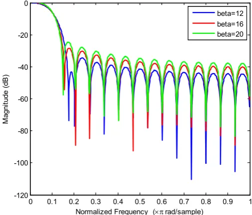
Figure 3 shows the frequency response characteristics of proposed window for a fixed

value of window length, N = 30. From Figure 1 it is clearly observed that for a fixed N

lower value of β results better minimum stopband attenuation (As) which is desirable.

At the same time it is incorporated with wider main-lobe half width. On the other side

minimum stopband attenuation. Thus for a given window length, higher values of β

results good mainlobe width and lower values of β results good minimum stopband

at-tenuation which maintains the contradictory nature of windowed filters. The

corres-ponding minimum stopband attenuation (As) and half main-lobe width (WR) for β =

12, 16, 20 are tabulated in Table 1.

From Table 1 it is observed that when β = 12, a minimum stopband attenuation

of −43.19 dB is obtained. If we increase β to 16, stopband attenuation becomes −28.40

dB and increasing β from 16 to 20 results a stopband attenuation of −26.18 dB. Thereby

we get better minimum stopband attenuation for lower values of β. But this lower β

re-sults worse mainlobe width which is undesirable. Again, increasing β from 12 to 20, the

normalized mainlobe width becomes narrower and narrower from 0.171 to 0.140. Table 2 shows some maximum values of stopband attenuation that results for a

giv-en window lgiv-ength. For example, whgiv-en N = 40, we are able to get a maximum value of

As = −104.27 dB which is more than enough for such a small window length in many

practical applications.

3.2. Relationship between Adjustable Parameter and Minimum

Stopband Attenuation

In the frequency domain, stopband attenuation is one of the most important parameter

Figure 3. Frequency response characteristics of proposed window.

Table 1. Characteristic values of proposed window.

N β As (dB) WR

30 12 −43.19 0.171

30 16 −28.40 0.154

30 20 −26.18 0.140

0 0.1 0.2 0.3 0.4 0.5 0.6 0.7 0.8 0.9 1

-120 -100 -80 -60 -40 -20 0

Normalized Frequency (×π rad/sample)

M

agni

tude (

dB

)

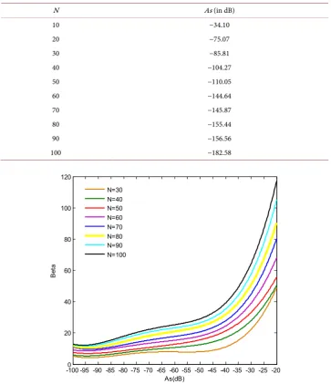
of a designed filter. Figure 4 shows the relationship between minimum stopband

at-tenuation (As) and adjustable parameter (β) for window length N = 30, 40, 50, 60, 70,

80, 90, 100.

For fixed values of N, a general approximate design relation between β and As can be

achieved using quadratic polynomial curve fitting method which is given by Equation (2). This equation will be very helpful for the designers who want to use this window

for a desired value of N and As.

4 3 2

aAs bAs cAs dAs e

β =

+

+

+

+

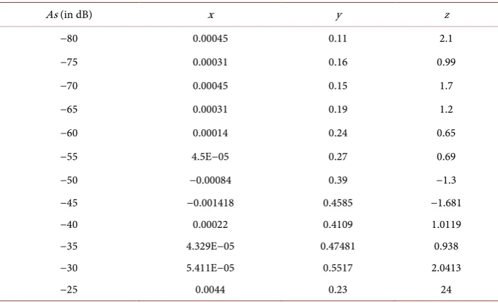
Values of co-efficients a, b, c, d, e in Equation (2) are given in Table 3 for N = 30, 40,

50, 60, 70, 80, 90, 100. We have taken the values of As = −20 dB, −25 dB, −30 dB, −35

Table 2. Maximum achievable values of As for some N.

N As (in dB)

10 −34.10

20 −75.07

30 −85.81

40 −104.27

50 −110.05

60 −144.64

70 −145.87

80 −155.44

90 −156.56

100 −182.58

Figure 4. The relationship between minimum stopband attenuation (As) and adjustable parame-ter (β).

-100 -95 -90 -85 -80 -75 -70 -65 -60 -55 -50 -45 -40 -35 -30 -25 -200

20 40 60 80 100 120

As(dB)

B

et

a

dB, −40 dB, −45 dB, −50 dB, −55 dB, −60 dB, −65 dB, −70 dB, −75 dB, −80 dB, −85

dB, −90 dB, −95 dB, −100 dB and obtained the corresponding values of β using

Equa-tion (2). From Figure 4 it is clear that in order to obtain a stopband attenuation of −100

dB we require approximate values of β = 5, 6, 7, 9, 11, 12, 13, 14 for N = 30, 40, 50, 60,

70, 80, 90, 100 respectively. Again we observe that for N = 30, a stopband attenuation

of −20 dB is obtained when β = 48 and a stopband attenuation of −100 dB is obtained

when β = 14.

3.3. Relationship between Adjustable Parameter and Window

Length

In some applications window length N is kept constant. To obtain an approximate

val-ue of β for a given N and As, windows of length N = 20, 30, 40, 50, 60, 70, 80, 90, 100

were designed to cover the range −25 dB ≤ As ≤ −80 dB. Figure 5 shows the plots of

Table 3. Approximate value of co-efficients appeared in Equation (2).

N a b c d e

30 8.85134E−06 0.0023954 0.24565 10.945 187.36

40 5.9548E−06 0.0016918 0.17729 8.2839 157.78

50 5.1347E−06 0.0014723 0.15769 7.6756 157.13

60 7.0379E−06 0.0020263 0.21601 10.314 203.08

70 9.612E−06 0.0027062 0.2815 13.084 249.42

80 1.122E−05 0.003149 0.32538 14.984 283.43

90 1.303E−05 0.0037011 0.38619 17.867 335.64

100 1.3884E−05 0.00397048 0.41821 19.529 370.09

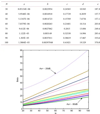
Figure 5. The relationship between window length, N and adjustable parameter, β.

20 30 40 50 60 70 80 90 100

0 10 20 30 40 50 60 70 80 90

N

B

et

a

As= - 25dB

window length N and adjustable parameter β. Using quadratic polynomial curve fitting

technique, an approximate design equation between β and N takes the general form,

2

xN

yN z

β =

+

+

Values of co-efficients x, y, z in Equation (3) for a range of As are presented in Table 4.

Figure 5 shows that for a small value of N, very small changes in β causes significant

changes in stopband attenuation. For example when N = 20, values of β = 10.5, 9.2, 7,

6.9, 6.2, 6.1, 5.5, 5.1, 4.9, 4.3, 4.2, 4.1, 3.8, 3.2, 3 results stopband attenuation of As = −30

dB, −35 dB, −40 dB, −45 dB, −50 dB, −55 dB, −60 dB, −65 dB, −70 dB, −75 dB, −80

dB, −85 dB, −90 dB, −95 dB, −100 dB respectively. But from it is also clear that As = −25

dB line is largely separated from other lines. This is because it is the lower limit of stopband attenuation that can be achieved by the proposed window. Again for some

applications if we choose N = 20 and want a value of As = −80 dB, we need to select β =

3 and if we choose N = 100 and want a value of As = −80 dB, we need to select β = 12

which is easily visible from Figure 5.

4. Performance Comparisons

In order to show the efficiency of proposed window, it is compared with well-known Cosh window and Exponential window. Although adjustable parameters of these two windows posses different characteristic values compared to the adjustable parameter of

our proposed window, for the sake of comparison, β of the proposed window is chosen

carefully that results a slightly better performance than the Cosh window and Exponen-tial window.

4.1. Comparison between Cosh Window and Proposed Window

Kaiser window has been derived by modifying the zero order Bessel function of first

Table 4. Approximate value of co-efficients appeared in Equation (3) for some desired As.

As (in dB) x y z

−80 0.00045 0.11 2.1

−75 0.00031 0.16 0.99

−70 0.00045 0.15 1.7

−65 0.00031 0.19 1.2

−60 0.00014 0.24 0.65

−55 4.5E−05 0.27 0.69

−50 −0.00084 0.39 −1.3

−45 −0.001418 0.4585 −1.681

−40 0.00022 0.4109 1.0119

−35 4.329E−05 0.47481 0.938

−30 5.411E−05 0.5517 2.0413

kind. This modified Bessel function exhibits the same shape characteristics as the Cosh

function. Thereby Cosh window has been defined as [8],

( )

( )

_{( )}

2

2

Cosh 1

1 _{0 1}

Cosh n N

w n n N

α

α

 

− _{ −} _

= ≤ ≤ − (4)

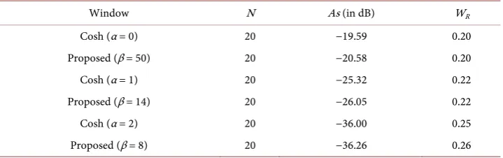
Table 5 shows the corresponding data of the two windows for window length N =

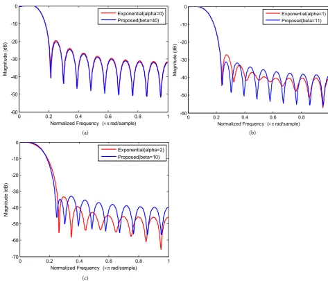
20. It is clear that, for different values of adjustable parameters α and β, the proposed

window provides slightly greater minimum stopband attenuation than Cosh window

for almost equal main-lobe half width. For example, when α = 0 and β = 50 our

pro-posed window results better minimum stopband attenuation and equal mainlobe half

width compared to Cosh window. The same performance is obtained for α = 1 and β =

14. But for α = 2 and β = 8 our proposed window remains superior in terms of stopband

attenuation only. Thus for higher values of β better performance of our proposed

win-dow is more significant.

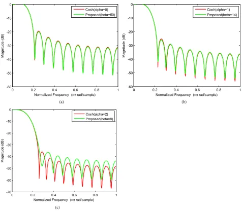
It is clearly observed from the Figures 6(a)-(c) that, for all pairs of α and β, our

proposed window results better minimum stopband attenuation and half mainlobe width simultaneously which is very rare for most of the existing window filters. For

small system (i.e., small window length N) the difference between characteristic values

obtained by Cosh and proposed window may not be significant enough but for larger

values of N it would be more advantageous to use our proposed window other than

Cosh window.

4.2. Comparison between Exponential Window and Proposed Window

The shape characteristics of zero order Bessel function is also similar to that of

expo-nential function. Hence Expoexpo-nential window has been defined as [7],

( )

( )

_{( )}

2

2

exp 1

1 1

exp 2

n

N N

w n n

α

α

 

−  ₋  ₋

 

= ≤ (5)

Figure 7 shows the frequency response characteristic comparison curve between Exponential window and proposed window. For all values of adjustable parameter, proposed window make a good compromise between the contradictory parameters

Table 5. Comparison data for Cosh window and proposed window.

Window N As (in dB) WR

Cosh (α = 0) 20 −19.59 0.20

Proposed (β = 50) 20 −20.58 0.20

Cosh (α = 1) 20 −25.32 0.22

Proposed (β = 14) 20 −26.05 0.22

Cosh (α = 2) 20 −36.00 0.25

(a) (b)

(c)

Figure 6. Characteristics comparison between Cosh window and proposed window for different values of α and β. (a) α = 0, β = 50; (b) α = 1, β = 14; (c) α = 2, β = 8.

namely stopband attenuation and mainlobe width. From Figure 7(b) and Figure 7(c)

better performance of our proposed window is easily visible.

Table 6 shows the resultant data obtained from the comparisons of exponential

window and proposed window for N = 20. From the tabulated data we observe that for

α = 0 and β = 90, proposed window provides both narrower main-lobe half width and

greater minimum stopband attenuation compared to exponential window. For α = 1

and β = 13, both of the windows have equal mainlobe half width but our proposed

window provides increased stopband attenuation. For α = 2 and β = 10, the resultant

stopband attenuation of proposed window is greatly increased while the mainlobe half

width is also reduced. For simplicity we take a small value of window length (N = 20).

But the result would be the same for larger values also.

From the data placed in Table 5 and Table 6, we conclude that for the same window

0 0.2 0.4 0.6 0.8 1

-60 -50 -40 -30 -20 -10 0

Normalized Frequency (×π rad/sample)

M

agni

tude (

dB

)

Cosh(alpha=0) Proposed(beta=50)

0 0.2 0.4 0.6 0.8 1

-60 -50 -40 -30 -20 -10 0

Normalized Frequency (×π rad/sample)

M

agni

tude (

dB

)

Cosh(alpha=1) Proposed(beta=14)

0 0.2 0.4 0.6 0.8 1

-70 -60 -50 -40 -30 -20 -10 0

Normalized Frequency (×π rad/sample)

M

agni

tude (

dB

)

(a) (b)

(c)

Figure 7. Characteristics comparison between exponential window and proposed window for different values of α and β. (a) α = 0, β = 40; (b) α = 1, β = 11; (c) α = 2, β = 10.

Table 6. Comparison data for exponential window and proposed window.

Window N As (in dB) WR

Exponential (α = 0) 20 −24.65 0.154

Proposed (β = 90) 20 −25.24 0.151

Exponential (α = 1) 20 −30.52 0.174

Proposed (β = 13) 20 −32.14 0.174

Exponential (α = 2) 20 −36.50 0.200

Proposed (β = 10) 20 −39.15 0.195

length N, our proposed window remains superior in terms of both stopband

attenua-tion and half mainlobe width. So our proposed can be a potential replacement for Cosh window and Exponential window for many important signal processing application

0 0.2 0.4 0.6 0.8 1

-60 -50 -40 -30 -20 -10 0

Normalized Frequency (×π rad/sample)

M

agni

tude (

dB

)

Exponential(alpha=0) Proposed(beta=40)

0 0.2 0.4 0.6 0.8 1

-60 -50 -40 -30 -20 -10 0

Normalized Frequency (×π rad/sample)

M

agni

tude (

dB

)

Exponential(alpha=1) Proposed(beta=11)

0 0.2 0.4 0.6 0.8 1

-70 -60 -50 -40 -30 -20 -10 0

Normalized Frequency (×π rad/sample)

M

agni

tude (

dB

)

where the length of the system cannot be increased (because this will increase the cost of the system) but better performance compared to the existing adjustable windows is required.

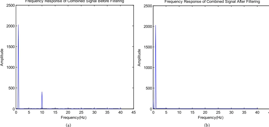
5. Filtering Performance of Proposed Window

In order to show the efficient performance of our proposed window, A MATLAB si-mulator is used to generate a signal 10cos (2πn) mixed with high frequency component

2cos (20πn + π/4) shown in Figure 8(a). Clearly, this signal has a frequency component

at 1 Hz and a frequency component at 10 Hz. If we want to eliminate the high frequen-cy component and the noise associated with it without affecting the low frequenfrequen-cy component, we must have to use a lowpass filter having a cutoff frequency above 1 Hz. Thus the mixed signal defined previously is applied to lowpass filter designed by using

our proposed window. A cutoff frequency of 1.5 Hz and a filter length of N = 10 has

been selected. Figure 8(b) shows that the high frequency component and the associated

noise above the cutoff frequency has been smoothly suppressed by our proposed win-dow filter. Moreover, the amplitude of the low frequency component in the filtered signal remains unchanged.

6. Conclusion

In this paper we have proposed an adjustable window function and its performance characteristics are evaluated using MATLAB simulator. For most of the windowed fil-ters, obtaining better minimum stopband attenuation is not possible without affecting the value of mainlobe half width. This contradictory behavior somehow limits the po-tential application of windowed filters. However our proposed window shows signifi-cant improvements in this regard. Within a particular range, this proposed window

(a) (b)

Figure 8. Filtration of high frequency signal by proposed window in the frequency domain: (a) before filtering; (b) after filtering.

0 5 10 15 20 25 30 35 40 45

0 500 1000 1500 2000 2500

Frequency(Hz)

A

m

pl

itude

Frequency Response of Combined Signal Before Filtering

0 5 10 15 20 25 30 35 40 45

0 500 1000 1500 2000 2500

Frequency(Hz)

A

m

pl

itude

provides better stopband attenuation without compromising the value of mainlobe width. This improved performance makes it suitable for practical applications such as medical imaging systems.

References

[1] Smith, S.W. (1999) The Scientist and Engineer’s Guide to Digital Signal Processing. 2nd Edition, California Technical Publication, 261-344.

[2] Bergen, S.W.A. and Antoniou, A. (2004) Design of Ultraspherical Window Functions with Prescribed Spectral Characteristics. EURASIP Journal of Applied Signal Processing, 13, 2053-2065. http://dx.doi.org/10.1155/S1110865704403114

[3] Rajput, S.S. and Bhadauria, S.S. (2012) Implementation of FIR Filter Using Adjustable Window Function and Its Application in Speech Signal Processing. International Journal of

Advances in Electrical and Electronics Engineering, 1, 158-164.

[4] Rajput, S.S. and Bhadauria, S.S. (2012) Comparison of Band-Stop FIR Filter Using Modified Hamming Window and Other Window Functions and Its Application in Filtering a Muti-tone Signal. International Journal of Advanced Research in Computer Engineering &

Technology (IJARCET), 1, 325-328.

[5] Bergen, S.W.A. and Antoniou, A. (2005) Design of Nonrecursive Digital Filters Using the Ultraspherical Window Function. EURASIP Journal on Applied Signal Processing, 12, 1910-1922. http://dx.doi.org/10.1155/ASP.2005.1910

[6] Samad, M.A. (2012) A Novel Window Function Yielding Suppressed Mainlobe Width and Minimum Sidelobe Peak. International Journal of Computer Science, Engineering and

In-formation Technology (IJCSEIT), 2, 91-103. http://dx.doi.org/10.5121/ijcseit.2012.2209

[7] Avci, K. and Nacaroglu, A. (2008) A New Window Based on Exponential Function. Pro-ceedings of the International Conference on Information & Communication Technologies:

from Theory to Applications, Damascus, Syria, 7-11 April 2008, 289-290.

http://dx.doi.org/10.1109/rme.2008.4595727

[8] Nouri, M., Ghaemmaghami, S.S. and Falahati, A. (2011) An Improved Window Based on Cosine Hyperbolic Function. Journal of Selected Areas in Telecommunications (JSAT), July Edition, 8-11.

[9] Basokur, A.T. (2011) Designing Frequency Selective Filters via the Use of Hyperbolic Tan-gent Functions. Bulletin of the Earth Sciences Application and Research Centre of

Hacet-tepe University, 32, 69-88.

[10] Basokur, A.T. (1998) Digital Filter Design Using the Hyperbolic Tangent Functions.