A Comparative Study of Feature Extraction and
Classification Methods for Iris Recognition
Thiyam Churjit Meetei
Department of Computer Science, Assam University,Silchar-788011, India
Shahin Ara Begum
Department of Computer Science,
Assam University, Silchar-788011, India
ABSTRACT
Iris recognition is one of commonly employed biometric for personal recognition. In this paper, Single Value Decomposition (SVD), Automatic Feature Extraction (AFE), Principal Component Analysis (PCA) and Independent Component Analysis (ICA) are used to extract the iris feature from a pattern named IrisPattern based on the iris image. The IrisPatterns are classified using a Feedforward Backpropagation Neural Network (BPNN) and Support Vector Machines (SVM) with Radial Basis Function (RBF) kernel with different dimensions and a comparative study is carried out. From the experimental result, it is observed that ICA is the most effective feature extraction method for both BPNN and SVM with Gaussian RBF for the consider datats. Futher, SVM with Gaussian RBF can classify faster than BPNN.
Keywords
Iris Recognition. image Segmentation. SVM. Classification.
1.
INTRODUCTION
A biometric recognition system can be used with a number of physiological characteristics (e.g. fingerprint, palmprint, hand geometry, face, iris, ear shape, and retina vein) and behavioral characteristics (e.g. gait, voice, signature and keystroke dynamics) to provide automatic recognition of individuals based on their inherent physical and /or behavioral characteristics. Among these biometrics, iris recognition is one of the most accurate and reliable biometric for identification because of following characteristics (i) Iris pattern has complex and distinctive pattern such as arching ligaments, crypts, corona, freckles, furrows, ridges, rings and a zigzag collarette [1]. (ii) possess 266 degrees-of-freedom in textural variability [2].
However, iris recognition also has disadvantages. Some parts of the iris are generally occluded by the eyelid and eyelash. The pupil and iris boundaries are not always circles and their centres are not concentric. If we approximate the boundaries of iris as circle, some parts of pupil and sclera may be present in the iris region. All these factors influence the performance of iris recognition system. To solve these problems, a robust recognition method is needed to remove the influence of all these noise as much as possible.
The modules of a typical iris recognition system are (i) Image acquisition deals with capturing iris images from the subject under a specifically setup scenario. (ii) Iris preprocessing and segmentation includes various steps such as iris localization by defining inner and outer boundaries of the iris, removal of occlusion of the eyelids and normalization. (iii) Feature extraction identifies the most discriminating features present in an iris pattern and the features are extracted to a pattern suitable for recognition. (iv) Last module is the matching or
classification which involves matching of input pattern(s) with stored patterns [3].
The present work includes image segmentation, feature extraction and classification. Iris segmentation is based on grayscale intensity of iris image. The iris pattern (IrisPattern) is formed by extracting features from segmented iris image by applying one of the four methods viz. SVD, PCA, AFE or ICA. The IrisPattern obtained is classified using Feedforward Backpropagation Neural Networks (BPNN) and SVM with Gaussian RBF kernel and a comparative study of the feature extraction and classification methods for iris recognition is carried out.
The rest of this paper is organized as follows: a brief review of literature is presented in Section 2. The present approach of iris segmentation and feature extraction are explained in Section 3. Experimental results and conclusions are presented in Section 4 and Section 5 respectively.
2.
LITERATURE REVIEW
competitive learning neural network (LVQ) for classification. Artificial neural network was used to classify iris patterns in [18],[19] [20]. SVM was also employed as classifier by many authors [3][14].
3.
IRIS RECOGNITION STEPS
The stages of iris recognition for the present work can be summarized as follow: (a) Iris segmentation, in which the iris is localized and segmented from iris image. (b) Feature extraction - Statistical methods, namely SVD, PCA, AFE and ICA are applied to reduce the dimension of IrisPattern (c) Classification accuracy is obtained by using BPNN and SVM with Gaussian RBF kernel in the experiment. The stages of the iris recognition system is shown in Figure 1. The Implementation details of the present work are explained in the following sub-sections.
Figure 1 Stages of the iris recognition system
3.1
Iris Segmentation
The main reason for the iris segmentation is twofold: (i) To extract only information i.e. the IrisPatterns that distinguishes individuals. (ii) To reduce the size of pattern vector from iris image to the IrisPatterns. Iris segmentation is carried out in following steps: detection of inner (papillary) boundary, outer boundary and isolation of IrisPattern from the iris image. The following algorithm for image segmentation is used in the present work:
3.1.1
Papillary Boundary Detection [21]
The input iris image is the eye region containing pupil, iris, sclera and eyelids. The pupil can be distinguishable in input image because it is consist of pixels with very low level intensity (black or almost black). A threshold is applied to find the pupil area as
( ) 70:1 0 : 70 ) ()
(
x
ff xxg
(1)where f is the original iris image and g is the thresholded image.
By applying this, all pixels with intensity higher than 70 (in a 0 to 256 scale) are set to 1 (black) and others are assigned to 0 (white). Some parts of eyelashes still present but have a much smaller area than the pupil area. All small regions other than pupil can be removed by applying code segment (2)
for each region R
if AREA(R) < 2500 (2)
set all pixels of R to 0
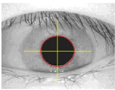
[image:2.595.376.494.69.161.2]Thus, pupil region is obtained. Two imaginary orthogonal lines are drawn passing through the centroid of the pupil region and by moving outwards from the centre, the first pixel with intensity zero is set as the boundaries of the binarized pupil. The output of this process is illustrated in Figure 2.
Figure 2 Detecting the Pupillary boundary
3.1.2
Iris Boundary Detection
The next step of iris segmentation finds the outer contour of the iris i.e. the iris-sclera boundary. The papillary and limbic boundaries of the eye are modeled as two concentric circles by many authors to reduce complexity [22]. Sometimes upper and lower parts of the iris may be occluded by the eyelid, as it is common with the Asians, and iris boundaries may not be circular. In some cases, iris centre and pupil centre may not coincide and the strips of iris may be of different width around the pupil.
To find iris outer contour, a horizontal imaginary line is drawn passing through the centre of the pupil that found out in 3.1.1. Starting from the edges of the pupil, the pixel intensity is analyzed outwards along the horizontal line and tries to detect sudden increase of intensity level on both side of pupil. Although the edge between the iris and the sclera is almost smooth, it is known that the iris region always has lower intensity than sclera. The difference of intensity levels is intensified by applying histogram equalization.
Edge detection of the iris image I(x, y) can be described as follows[21]:
I. Draw a horizontal imaginary line (H) passing through the centre (xcp, ycp) of the pupil. rx is horizontal radius of
the pupil.
II. Apply histogram equalization on image I(x, y): G(x, y) =histeq( I(x, y)).
III. Store the pixel intensities of the row passing through the pupil centre (xcp, ycp) of G(x, y)in a vector V={v1, v2, …,
vw} where w is the width of enhanced image G(x, y). IV. Create two vectors R={rxcp + rx, rxcp+rx+1, …, rw} and
L={lxcp-rx, lxcp-rx-1, …, r1} from line H on right and left
side of pupil respectively. Vector R is consist of the elements of the line H that start at the right edge of the pupil (rxcp + rx) and end at the width (w) of the image.
For vector L, it ranges from the left edge of the pupil (rxcp - rx) to the first element of line H.
V. For both vectors R and L:
a. Create the average window vector AvgW={a1, …,
an} where n=|L| or n=|R|. Vector AvgW is
subdivided in i windows of size ws. For all window ws
n
i
1/ , elements ai.ws-ws … ai.ws will contain theaverage of that window.
In our experiments, a window size ws=10 provides satisfactory results.
b. Identify the point that gives the first increase of values in Aj(1 ≤ j ≤ n) that exceeds a set threshold
d. In our experiments, a value of d equal to 18 has shown to identify the correct location of the iris edge.
VI. Calculate outer radii of iris IR and IL on both sides. If IR Iris Segmentation
Pattern Classification Feature Extraction
Classn Match Unknown
≤ 80 or 150 ≤ IR then IR = IL and vice versa. We make this assumption because the iris images in CASIA-IrisV1 database has iris radius 80 to 150 [16].
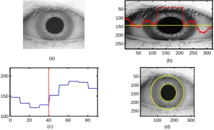
The time complexity is O (m.n) for the histogram equalization of an image of size mn, and O (m) for edge finding. Total time complexity is O (m.n). The iris segmented results obtained from an iris image from CASIA-IrisV1 database is shown in Figure 3. The algorithm is based on variation of local intensity and computes fast. While testing against iris images from CASIA-IrisV1 database, the algorithm gives a satisfactory result of 723 successes (95.64%) and 33 failure (4.36%) out of 756 images. From the analysis of the failure cases, it is found that sclera was not as white as expected or thick eyelashes were around the iris.
(a)
(b)
50 100 150 200 250 300 50
100 150 200 250
0 20 40 60 80
100 150 200
(c) (d)
100 200 300 50
[image:3.595.318.540.210.302.2]100 150 200 250
Figure 3. Iris edge detection (a) Original image (b) Enhanced image using Histogram equalization, yelow line passes through centre of pupil of image, zig-zag line shows
pixel intensities along horizontal line. (c) Averaged intensities of pixels along horizontal linefor right side of
the pupil (d) Iris image with boundaries
3.1.3
Forming IrisPattern
Segmentation is formation of IrisPattern by isolating only information that distinguishes individuals and also to reduce the dimensionality of the problem by extracting areas of the iris at the left and right sides of the pupil. By avoiding the intra-class rotation of iris images, an IrisPattern (m n) is extracted from iris image (320280) where m n is the required dimension of IrisPattern. The overall algorithm can be summarized as follows [21]:
I. Retrieve pupil centre and radius.
II. Retrieve iris endpoints.
III. Calculate rows spacing s = pupil diameter / m where m is required number of IrisPattern rows.
IV. Calculate the first target row index = |centre of pupil – vertical pupil radius|.
V. For both the sides of the pupil, perform the followings:
a. Compute baseline width = |iris edge of current side – pupil edge of current side|.
b. Starting from the top of the pupil to the bottom with a spacing of s, conduct the following steps for all baselines:
i) By using the equation of circle, locate the pixel point (x, y) that resides in the intersection of the circle centre at pupil centre with radius equal to pupil radius and current baseline.
ii) Vector B is appended with n/2 pixels that are under the baseline. Calculate pixel intensity by taking average mask of 33 pixels.
iii)Append vector B to IrisPattern matrix of respective side of the iris.
VI. The two halves of IrisPattern matrices are merged side by side into one final IrisPattern matrix.
Present method takes in consideration only the areas of iris on the left and right of the pupil at to data extraction because these areas are the ones that most often visible in an iris image. The areas above and below the pupil possesses unique information but generally they are partially or totally occluded by eyelid or eyelash. This approach reduces removal of occlusion by eyelid or eyelash. Figure 4 shows the output of the strategy.
(a) (b)
20 40 60 80 100 120
20
40
60
80
[image:3.595.60.274.231.361.2]100
Figure 4 IrisPattern (a) Iris with IrisPattern (b) Isolated
IrisPattern
3.2
Feature Extraction
The signals (or images) captured by sensory systems generally contain high redundant information and if not summarized or filtered, it would bottleneck the whole process of pattern recognition and classification. Therefore, dimensionality reduction (i.e. feature extraction or selection) is one of the most importance step in pattern recognition problems. We can apply mathematical and statistical methods (such as ICA, PCA, Wavelets and Fourier Transforms) to reduce the dimensionality of the problem.
The CASIA-IrisV1 database provides images of 320280 pixels and one image is equivalent to a vector with 89,600 elements. Classification of these vectors needs too high computing power, and still may not guarantee satisfactory results. During iris segmentation, dimension reduction was already achieved by simply isolating the area of the iris image that contains the characteristic information about an individual. For instance, we decrease the number of elements in the input vector from 89,600 (320280 image) to 1600 (4040 images), a 98% reduction in size. Still a large percentage of redundant information are contained in IrisPatterns, mathematical and statistical methods can be employed to reduce the dimensionality of the problem. This problem is also known as feature extraction, from a set of n features, select a set of m most prominent features that leads to to reduce the dimensionality as well as to minimum classification error. Single Value Decomposition (SVD), Principal Component Analysis (PCA), Automatic Feature Extraction (AFE) and Independent Component Analysis (ICA) are applied to IrisPattern for this purpose.
3.2.1
Single Value Decomposition
(SVD)SVD is a powerful technique in matrix computation and analysis, and noise signal filtering etc.. SVD is related to the rank of a matrix and it has an ability to approximate matrices of a given rank. In the present work, SVD is employed as a signal filter to reduce dimension of IrisPattern.
T
USV
A
(3)where the superscript “T” denotes matrix transpose. U is an m m orthogonal matrix, V is an n n orthogonal matrix and S is an m n diagonal matrix with sij = 0 if i ≠ j and sii ≥ si+1 i+1. The columns of U and those of V are left and right singular vectors respectively. SVD reduces the dimension of input pattern from m n to only a vector of n elements. The first n elements contain substantial information, and the vector tail can be cropped up without significant loss of generality.
3.2.2
Principal Component Analysis (PCA)
PCA is a useful statistical technique that aims to find a linear orthogonal transformation v = Wu (where u is the observation vector) such that the maximum amount of variance possible by n linearly transformed components can be retained. Mathematically, PCA is the method of the eigenvalue decomposition of the covariance matrix [24].
Let A be a square symmetric nn matrix, and consider its eigenvalue decomposition
n i T i i i Tp
p
P
P
A
1
(4)where P is an orthogonal matrix with columns p1, …, pn and is a diagonal matrix with eigenvalues λ1, λ2, ···, λn which are
sorted in descending order. pi is the eigenvector corresponding
to eigenvalue λi.
A simple approach to PCA is to use singular value decomposition (SVD). Let n m-dimensional vectors Xj is
aligned in the data matrix X (m n) and C is the covariance matrix of X. Then, SVD (C) will be the PCA of X.
3.2.3
Automatic Feature Extraction (AFE)
Automatic Feature Extraction is based on Nyström approximation method. Nyström method is an approximation based on the numerical integration in integral equations. Theoretically, this method analyzes non-uniform distributions but it is commonly used with uniform sampling without replacement [25]. It is an effective tools for a variety of large-scale learning applications, in particular in dimensionality reduction and image segmentation.
Consider the eigenfunction problem:
D D t t ds s s tK(. ) ( ) ( ), (5)
where K(t,s) is kernel, Ф eigenvector, Let D = [a, b] . All points in D are interpolated with the quadrature rule
b
a
n
j
w
jy
s
jds
s
y
1
(
)
)
(
(6)where {wj} are the weights and {sj} are the quadrature
points. Then (5) becomes
)
(
~
)
,
(
)
(
)
.
(
1 j D nj
w
jk
x
s
js
ds
s
s
t
K
(7)which leads to an eigenvalue problem of the form
) ( ~ ~ ) ( ~ ) , (
1w k x s sj x
n
j j j
(8)The approximate eigenvalue
~ and approximate eigenfuction ~ for x = xi,i = 1, …, n can be found out withthe Nyström method as
)
(
~
~
)
(
~
)
,
(
1 j i
n
j
w
jk
x
s
j
s
x
(9)that depend on the set {xi} of Nyström points. If
~
m
0
, the exact eigenvectorsm
~ on the Nyström points can be extended to a function
) ( ~ ) , ( 1 ) ( 1 j n
j j j
m
m x
w k x s s
(10)The function (x)
m
is the Nyström extension of the eigenvector
m
~ , and can be calculated for a (small) number n of points in the (large) full domain D.
3.2.4
Independent component analysis (ICA)
Independent component analysis (ICA) is a statistical technique that represents a multidimensional source vector as a linear combination of non-gaussian random independent variables called independent components [26]. It aims to capture the independent sources in order to analyse the underlying randomness of the observed signals.
Mathematically, it is convenient to use matrix notation. Let random (source) vector s = (s1, …, sn) and (mixed) random
vector x = (x1, …, xm). Let A be a (mixed) matrix with
elements aij , i = 1, ..., m, j = 1, ..., n.
Ax
s
(11)where maximally independent components (x1, …, xm)
measured by some function F (s1, …, sn) of independence.
The model in (11) is called independent component analysis or ICA model.
ICA is dependent on the correlation information among input patterns and preprocessing is needed to obtain reasonable results. Preprocessing includes centering and whitening the mixing matrix as well as the independent components. Also, the output dimensions is to be decided prior to processing as reduction is done automatically in the algorithm. In order to obtain the independent components using FastICA algorithm [27], the following arrangements are necessary:
I. Given the input image Imn, pixels of the image are arranged by concatenating m rows of n columns into a pattern vector of (m n) columns.
II. Given the data set Dl of L cases, the training set would
have L rows and m n columns. For supervised learning, there is one additional label column labeling the case, making the length of the pattern vector as m n + 1.
III. Then, transpose the dataset to feed into FastICA algorithm.
3.3
Pattern Classification
3.3.1
Backpropagation Neural Network (BPNN)
A 3-layer BPNN is employed in the present work (Figure 5). Number of neurons in the input layer is equal to the dimension of the IrisPattern. As a rule of thumb, number of neurons in the hidden layer should be approximately double of the neurons in the input layer. The number of neurons in the output layer is equal to the number of classes to be recognized. For example, if it is to classify iris images into 50 classes, there should have 50 output neurons in the network.
Figure 5 BPNN
In supervised training mode, a target vector T is feed into the network. In this target vector T, every element is set to zero, except on the position of the target class which is set to 1. For each input pattern X, an output vector Y is generated by the network which has number of elements equal to that of output neurons. Each output neuron processes a squashing function that produces a real number in the range [0, 1]. To determine the winner class indicated by the network, the maximum number in Y is selected and set it to 1, while setting all other elements to zero. The element set to 1 indicates the classification of that input pattern.
3.3.2
Support Vector Machines (SVM) with RBF
kernel
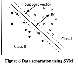
The foundations of SVM have been developed by Vapnik in 1995 [28]. The SVM method was originally developed as a linear classifier. Later, it was extended to allow non-linear mapping of data to the feature space by using kernel methods. The principle of data separation using SVM is demonstrated on a simplified linear example in Figure 6.
Figure 6 Data separation using SVM
A linear SVM classifier is defined as [29]
0
)
.
(
W
x
b
(12)where W is hyperplane’s normal vector, b is offset and b/|W| is the perpendicular distance from the hyperplane to the origin.
The distance of the decision surface (or hyperplane) (solid line in Figure 6) from the nearest appearance of the individual data sets should be made as large as possible. The dashed lines (in Figure 6) that are parallel with the decision surface
contain support vectors. The minimal distance of a sample to the hyperplane is defined as the margin.
For a linearly separable data, a matrix H is created by dot product of input variables as
) ( i j j i ij yyk xx
H (13)
where yi∈{1, -1}; xi, xj are data points from the original
space and k(xi.xj) is called Kernel Functions. By using Kernel
Functions, a non separable dataset in the input space x can be mapped into a higher dimensional feature space to make it seperable.
In the present work, Gaussian RBF (radial basis function) kernel is used. RBF kernel is given by
k(xi.xj) = exp(-| xi - xj|
2
/c), c > 0 (14) where c is a penalty parameter of the error. It is important to optimize parameter c to optimize the solution.
4.
EXPERIMENTAL RESULTS
In the present work, we use the CASIA-IrisV1 database collected by the Chinese Academy of Sciences’ Institute of Automation [30]. The database consists of 108 (iris) classes. For each class, there are 7 sample images taken in two sessions, three samples taken in the first session and four samples taken in the second. Total number of iris images is 756. Size of Images are 320280 pixels gray scale taken by a digital optical sensor designed by NLPR (National Laboratory of Pattern Recognition – Chinese Academy of Sciences).
At stage of the iris segmentation, window technique and the grayscale intensity based algorithm is applied. Experiments are conducted in Matlab 7.9 environment. The accuracy rate was 95.64% for iris segmentation and average time taken was 0.13s.
In classification stage, the iris patterns are classified using BPNN and SVM with RBF kernel. The network design parameters of the present experiment is summarized as:
Training function : traingda
Initial learning rate : 0.15 Learning rate increment : 1.05
Epochs : 50,000
Error goal : 0.0000000001
Minimum gradient : 0.0000000001
IrisPattern of 50 persons/classes (i.e. 350 images) from CASIA-IrisV1 database is used in this experiment. IrisPattern is 40×40 pixels with an average mask of 3×3 pixels. The outputs of the neural network are classes of iris patterns. Each class characterizes a person’s iris. The training dataset is consist of five instances of each class and the remaining two instances of each class are used for testing.
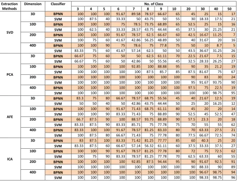
The performance of the four feature reduction methods with different dimensions and different number of classes are analysed using BPNN and SVM with RBF. The recognition method that generates the best classification performance is ranked the best. The best classification accuracy rate (%) of ten times execution is shown in table 1 with four different dimensions (i.e. 3D, 10D, 20D and 40D) against twelve different classes (i.e. 3, 4, 5, 6, 7, 8, 9, 10, 20, 30, 40 and 50) by using both classifiers. From the experimental result, it is observed that higher the number of classes decreases the correct classification rate in both cases (except some cases). Performance of both classifiers with SVD, PCA or AFE are poor in higher number of classes (i.e. more than 20) and lower
X1
X2
X3 . . .
Xm
Y1
Y2
Y3
. .
Yn
.
.
.
.
.
.
h1
h2
h3
h4
hl
W Support vector
Class I
[image:5.595.86.247.516.651.2]dimension (i.e. 3 D), therefore these combinations perhaps cannot be applied for classes above 20 with low dimension. And also BPNN shows its highest classification results only with ICA except 3D. On the other hand, SVM with RBF performs better with PCA or ICA (except some cases) than with SVD or AFE and it also works better than BPNN in higher number of classes. ICA is the best feature extraction method among the four methods for both BPNN and SVM with RBF.
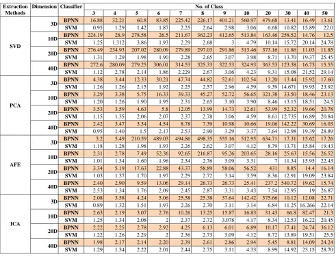
The time taken in classification (in sec) by the two classifiers with four different extraction methods at different dimensions and classes is shown in table 2. Experimental observations show that BPNN can classify faster with PCA or ICA than with SVD or AFE. SVM with RBF takes longer time in classification for higher number of classes than at lower number of classes in all extraction methods and can classify faster than BPNN.
5.
CONCLUSION
[image:6.595.56.543.280.654.2]Iris recognition system using BPNN and SVM classifiers is presented in this paper. A window technique based iris segmentation is implemented and average segmentation time is 0.13s. It is possible to choose an output dimension of the IrisPattern smaller than its original size by extracting areas of the iris at the left and right of the pupil. In this approach, removal process of occlusion by eyelash or eyelid in iris recognition is reduced. Four statistical methods namely SVD, PCA, AFE and ICA are applied separately to extract features from IrisPattern. Two classifiers viz. BPNN and SVM with RBF are employed to classify IrisPattern. From the experimental results, it is observed that the performance of ICA is obvious with both classifiers, as classification results are very good with the 40D experiment. And SVM with RBF can classify faster than BPNN.
Table 1. Comparison of the classification rate (%) of BPNN and SVM with RBF
Extraction Methods
Dimension Classifier No. of Class
3 4 5 6 7 8 9 10 20 30 40 50
SVD
3D BPNN 100 100 100 91.67 89.58 78.57 66.67 65 45 25 15 17
SVM 100 87.5 40 33.33 50 43.75 50 55 30 18.33 17.5 21
10D BPNN 100 100 100 75 78.5 73.75 68.89 65 52.5 25 15 16
SVM 100 62.5 40 33.33 28.57 43.75 44.44 45 37.5 30 21.25 21
20D BPNN 100 100 100 91.67 78.57 62.5 66.67 60 42.5 16.67 11.25 7
SVM 100 75 60 41.67 42.86 56.25 48.89 50 40 31.67 20 16
40D BPNN 100 100 90 75 78.6 75 77.8 75 50 10 8.7 5
SVM 83.33 75 60 41.67 57.14 62.5 50 50 43.5 36.67 31.25 26
PCA
3D BPNN 66.67 75 60 50 50 62.5 61.11 70 22.5 21.67 7.5 15
SVM 66.67 75 60 50 42.86 50 55.56 45 32.5 28.33 26.25 27
10D BPNN 100 100 100 100 92.85 100 88.88 95 90 35 21.2 19
SVM 100 100 100 100 100 87.5 85.7 85 87.5 81.67 75 67
20D BPNN 100 100 100 100 100 100 100 100 90 83 30 24
SVM 100 100 100 100 100 100 100 100 95 91.67 93.75 90
40D BPNN 100 100 100 100 100 100 100 100 97.5 75 22.5 19
SVM 100 100 100 100 100 100 100 100 100 100 98.75 95
AFE
3D BPNN 83.3 75 80 66.67 78.57 68.75 55.56 45 40 21.67 12.5 19
SVM 50 50 40 50 42.86 43.75 44.44 50 25 20 16.25 12
10D BPNN 100 100 90 91.67 71.43 68.75 61.11 80 45 20 20 14
SVM 100 100 90 83.33 71.43 75 88.89 90 52.5 45 52.5 47
20D BPNN 66.7 87.5 90 100 88.57 93.75 88.89 90 57.5 23.3 20 18
SVM 83.33 87.5 90 83.33 85.71 75 77.78 75 70 55 55 62
40D BPNN 83.33 100 100 91.67 78.57 81.25 83.33 80 70 63.33 27.5 21
SVM 100 87.5 80 66.67 71.43 75 77.78 80 77.5 66.67 72.5 74
ICA
3D BPNN 83 87.5 100 83.33 71.42 81.25 77.77 85 60 40.3 25 20
SVM 83.33 87.5 60 66.67 57.14 56.32 61.11 60 37.5 33.33 37.5 27
10D BPNN 100 100 90 91.67 78.57 81.25 77.78 80 72 75 72.5 62
SVM 100 75 90 83.33 78.57 81.25 77.78 70 62.5 63.33 60 55
20D BPNN 100 100 100 100 92.85 87.5 94.44 95 90 91.67 92.5 91
SVM 100 100 100 100 100 100 100 100 90 88.33 90 89
40D BPNN 100 100 100 100 100 100 100 100 100 96.67 98.75 94
Table 2 Classification time taken (in sec) by BPNN and SVM with RBF
Extraction Methods
Dimension Classifier No. of Class
3 4 5 6 7 8 9 10 20 30 40 50
SVD
3D BPNN 16.88 32.21 60.8 83.85 225.42 226.17 401.21 560.97 479.68 13.41 16.49 13.61
SVM 0.95 1.29 1.42 1.87 2.25 2.64 2.98 3.06 6.68 10.82 15.89 22.0
10D BPNN 224.19 28.9 278.58 26.5 211.67 362.23 412.65 513.84 163.46 258.52 14.76 12.5
SVM 1.25 1.312 3.86 1.93 2.29 2.68 3 4.79 10.14 15.72 20.14 24.78
20D BPNN 276.49 234.93 207.02 280.09 279.89 297.03 291.86 313.46 373.16 11.86 11.03 11.85
SVM 1.31 1.29 1.98 1.90 2.28 2.65 3.07 3.98 8.71 13.70 19.37 25.45
40D BPNN 272.6 280.09 279.25 306.01 314.53 325.33 322.53 324.93 363.53 123.38 16.73 15.55
SVM 1.12 2.78 2.14 1.86 2.229 2.67 3.06 4.23 9.31 15.08 21.52 29.14
PCA
3D BPNN 4.38 3.44 12.33 30.21 47.74 44.82 52.61 102.54 13.20 13.44 15.92 17.60
SVM 1.26 1.26 2.15 1.92 2.25 2.57 2.96 4.59 9.39 14.671 19.95 23.92
10D BPNN 3.29 3.38 5.75 16.33 39.33 45.27 52.72 56.65 321.38 33.50 18.46 23.13
SVM 1.20 1.26 1.90 1.95 2.31 2.65 3.10 3.90 8.46 13.15 18.51 24.5
20D BPNN 3.53 3.59 4.63 5.8 12.05 13.99 14.73 12.61 53.99 52.32 19.66 20.78
SVM 1.15 1.35 2.06 2.07 2.37 2.78 3.06 4.59 8.61 12.735 16.89 20.84
40D BPNN 2.42 3.47 3.34 4.54 8.78 7.39 10.98 10.66 19.06 142.22 30.69 16.03
SVM 0.95 1.40 1.5 2.17 2.53 2.90 3.29 3.37 7.64 12.98 19.39 28.89
AFE
3D BPNN 3.2 5.49 210.59 489.03 494.86 498.35 555.16 512.95 634.71 17.31 15.62 17.26
SVM 1.18 1.28 1.98 1.93 2.26 2.62 3.07 4.12 8.79 13.71 15.84 19.43
10D BPNN 2.31 2.78 7.49 52.36 92.65 216.87 95.26 203.65 28.16 25.63 15.56 26.52
SVM 1.01 1.34 1.60 1.96 2.34 2.76 3.09 3.31 7 11.34 15.95 22.43
20D BPNN 3.34 5.19 17.63 22.88 43.37 58.89 58.06 56.52 431 8.85 14.4 16.14
SVM 1.03 1.37 1.70 1.97 2.29 2.72 3.14 3.59 8.36 12.91 19.09 23.84
40D BPNN 2.40 2.90 9.59 13.06 29.14 26.73 26.73 25.41 237.2 540.72 19.62 15.74
SVM 2.53 1.34 1.76 2.09 2.45 2.87 3.31 3.43 7.54 12.95 19 26.87
ICA
3D BPNN 2.08 3.58 4.24 5.06 25.58 25.38 37.64 142.42 575.66 10.12 12.08 22.71
SVM 0.89 1.32 1.51 1.93 2.26 2.70 3.11 3.14 6.84 11.25 16.266 22.14
10D BPNN 2.63 2.19 3.07 2.76 10.26 13.25 15.87 16.83 31.43 66.8 82.47 21.3
SVM 1.25 1.34 2.08 2 2.37 2.72 3.078 4.17 8.34 12.53 16.22 20.45
20D BPNN 2.22 2.25 2.78 2.92 4.25 6.13 6.01 6.89 10.17 17.41 24.74 36.12
SVM 1.22 1.26 2.29 2 2.36 2.73 3.09 4.12 8.72 13.89 19.51 25.5
40D BPNN 1.98 2.17 2.14 2.20 2.39 2.61 2.86 2.94 5.45 8.81 14.09 24.24
SVM 1.29 1.34 2.22 2.01 2.44 2.75 3.11 4.33 8.99 14.92 23.15 28.70
6.
REFERENCES
[1] Daugman J. 2004. How Iris Recognition Works. IEEE Transactions on Circuits and Systems for Video Technology, 14(I):21-30
[2] Daugman J. 2002. Recognizing Persons by Their Iris Patterns. The Computer Laboratory, University of Cambridge, UK
[3] Li M., Tieniu T., Yunhong W. and Dexin Z. 2003. Personal Identification based on Iris Texture Analysis. IEEE Transactions on Pattern Analysis and Machine Intelligence 25(12):1519 – 1533
[4] Wildes R. 1997. Iris Recognition: an Emerging Biometric Technology. Proc. IEEE, 85(9):1348-1363
[5] Lim S., Lee K., Byeon O. and Kim T. 2001. Efficient Iris Recognition through Improvement of Feature Vector and Classifier, J. ETRI 23(2):61-70
[6] Liu Y., Yuan S., Zhu X. and Cui Q. 2003. A practical iris acquisition system and a fast edges locating algorithm in iris recognition. IEEE Instrumentation and Measurement Technology Conference, pp. 166–168
[7] Zhaofeng H., Tieniu T. and Zhenan S. 2006. Iris Localization via Pulling and Pushing, Int. Conference on Pattern Recognition, pp. 366 – 369
[8] Kong W. and Zhang D. 2001. Accurate Iris Segmentation Based on Novel Reflection and Eyelash Detection Model. Proc. ISIMVSP, pp. 263–266
[9] Boles W. and Boashash B. 1998. A human Identification Technique Using Images of the Iris and Wavelet Transform. IEEE Transactions On Signal Processing 46(4):1185-1188.
[10]Ma L., Tan T., Wang Y. and Zhang D. 2004. Efficient Iris Recognition by Characterizing Key Local Variations. IEEE Trans. Image Processing 13(6):739-750
[11]Monro DM., Rakshit S. and Zhang D. 2007. DCT-Based Iris Recognition. IEEE Transactions on Pattern Analysis and Machine Intelligence 29(4):586-595
[12]Huang Y., Luo S. and Chen E. 2002. An efficient iris recognition system. Int. Conference of Machine Learning and Cybernetics, 1:450–454
[13]Dorairaj V., Schmid N. and Fahmy G. 2005. Performance Evaluation of Iris Based Recognition System Implementing PCA and ICA Techniques. Proc. SPIE 5779: Biometric Technology for Human Identification II, 5779:51–58
[15]Chitte PP, Rana JG, Bhambare RR, More VA, Kadu RA and Bendre MR. 2012. IRIS Recognition System Using ICA, PCA, Daugman’s Rubber Sheet Model Together. Int. J. Computer Technology and Electronics Engineering (IJCTEE), 2(1):16-23
[16]Chandra Murty PSR and Reddy ES. 2009. Iris Recognition system using Principal Components of Texture Characteristics. TECHNIA-Int. J. Computing Science and Communication Technologies, 2(1): 343-348
[17]Rashad MZ, Shams MY, Nomir O and El-Awady RM. 2011. Iris Recognition Based on LBP And Combined LVQ Classifier. Int. J. Computer Science & Information Technology (IJCSIT) 3(5):68-78
[18]Abiyev RH and Altunkaya K. 2008. Personal Iris Recognition Using Neural Network. Int. J. Security and its Applications 2(2): 41-50
[19]Araghi LF, Shahhosseini H. and Setoudeh F. 2010. IRIS Recognition Using Neural Network. Proc. Int. MultiConference of Engineers and Computer Scientists 2010 Vol. I, Hong Kong
[20]Wagdarikar AMU, Patil BG and Subbaraman S. 2010. Performance Evaluation of IRIS Recognition Algorithms using Neural Network Classifier. IEEE, 978-1-4244-5539-3/10
[21]Merloti PE. 2004. Experiments on Human Iris Recognition Using Error Backpropagation Artificial Neural Network. Dissertation, San Diego State University.merlotti.s465.sureserver.com/EngHome/Com puting/iris_rec_nn.pdf. Accessed 16 Aug 2010
[22]Kevin WB, Hollingsworth K. and Patrick JF. 2008. Image Understanding for Iris Biometrics: A Survey. Computer Vision and Image Understanding, 110(2): 281-307
[23]Akritas AG, Malaschonok GI and Vigklas PS. 2006. The SVD-Fundamental Theorem of Linear Algebra. Nonlinear Analysis: Modelling and Control 11(2): 123– 136
[24]Jolliffe I. T. 2002. Principal Component Analysis. Spinger-Verlag, NY, 2nd Ed.
[25]Drineas P and Mahoney MW. 2005. On the Nyström Method for Approximating a Gram Matrix for Improved Kernel-Based Learning. J. Machine Learning Research, 6:2153–2175
[26]Hyvärinen A and Oja E. 2000. Independent Component Analysis: Algorithms and Applications. Neural Networks, 13(4-5):411-430
[27]FastICA 2005. FastICA Matlab package. http://www.cis.hut.fi/projects/ica/fastica. Accessed 26 Aug 2010
[28]Bishop CM 2006. Pattern Recognition and Machine Learning. Springer Science and Business Media, LLC, NY
[29]Müller KR, Mika S., Rätsch G., Tsuda K. and Schölkopf B. 2001. An Introduction to Kernel-Based Learning Algorithms. IEEE Transactions on Neural Networks 12(2):181-201