Munich Personal RePEc Archive
Technology Shocks and Hours Worked:
Checking for Robust Conclusions
Whelan, Karl
University College Dublin, School of Economics
October 2006
Technology Shocks and Hours Worked:
Checking for Robust Conclusions
Karl Whelan
Central Bank and Financial Services Authority of Ireland∗
October 2006
Abstract
This paper presents some new results on the effects of technology shocks on hours worked based on structural VAR specifications containing various measures of US pro-ductivity growth and hours. These specifications can produce different answers depend-ing on which sector of the economy is examined, which transformation of hours worked is used, and on how many lags are chosen for the VAR. However, it is shown that the re-sults from the stochastic trend specification used by Jordi Gal´ı (1999) are robust across changes in data definition and lag length, while the results from the per capita hours specification of Christiano, Eichenbaum, and Vigfusson (2003) are not. These results provide support for Gal´ı’s findings that technology shocks have a negative impact effect on hours worked and that these shocks play a limited role in generating the business cycle.
1
Introduction
The relative merits of flexible-price real business cycle (RBC) models and sticky-price New-Keynesian models in explaining macroeconomic phenomena is perhaps the central contro-versy in modern macroeconomics. And the issue of how technology improvements affect the labor market has become an important testing ground for assessing the relative merits of these two approaches: Standard RBC models predict that positive technology shocks should generate a short-run increase in hours worked, while Keynesian models with output determined by aggregate demand can predict that such shocks temporarily reduce hours. Against this background, Jordi Gal´ı’s (1999) demonstration using a structural VAR that positive technology shocks produce a short-run decline in hours worked has been promi-nently cited as an important piece of evidence against the RBC approach.1
But Gal´ı’s conclusions have not been universally accepted. In particular, Christiano, Eichenbaum, and Vigfusson (2003, henceforth CEV) argue that findings of a negative effect of technol-ogy shocks on hours worked are solely driven by a faulty handling of the trend component of hours worked. Gal´ı’s analysis deals with the upward trend in hours worked by assuming either the existence of a deterministic trend or of a stochastic trend such that the log-difference of hours is stationary. CEV argue instead for analyzing hours on a per capita basis and show that when this series is used, positive technology shocks appear to boost hours in the short run.
In this paper, I present some new results based on structural VAR specifications con-taining various measures of US productivity growth and hours. These results show that Gal´ı’s preferred approach produces far more robust results than CEV’s approach. In par-ticular, results from specifications using per capita hours turn out to be highly sensitive to the particular data series for hours chosen and to the number of lags used in the VAR analysis. For example, CEV’s results relate to a VAR for the business sector with four lags, but do not hold for VARs using the definition of hours used in Gal´ı’s study (which relates to the nonfarm business sector) and shorter lag lengths (as chosen by lag-selection tests). In contrast, the results for Gal´ı’s stochastic trend approach turn out to be robust across all of the various data definitions used for hours and productivity and across all lag lengths tested—and in all cases, these results suggest that a positive technology shock has
1
a significant negative impact effect for on hours worked.
Given that we would hope that a reliable methodology for the measurement of the labor market effects of technology shocks would not prove sensitive to minor changes in specification, such as a slight change in the definition of hours or in the number of lags used, these results point towards Gal´ı’s stochastic trend specification as being preferable to the approach of CEV. Importantly, these specifications also point to technology shocks playing a very limited role in generating the business cycle components of hours and output. The contents of the rest of the paper are as follows. Section 2 briefly reviews the methodology used to identify technology shocks and their effects on hours and output. Section 3 presents the results. Finally, Section 4 assesses the various specifications and methodologies for detrending hours.
2
Methodology
I follow the methodology adopted by Gal´ı (1999) to identify technology shocks and their effects on hours and output. The first step is the estimation of a reduced-form VAR featuring the growth rate of labor productivity and some transformation of hours worked. Denote the log of labour productivity byztand the log of hours bynt. Consider now the inverted Vector
Moving Average (VMA) representation of a reduced-form VAR featuring the log-differences of labor productivity and hours:
Xt=
∆zt
∆nt
=A(L)vt (1)
whereA(0) =I and E(vtv′
t) = Σ. Gal´ı’s identifying assumptions are that productivity and
hours are driven by two independent structural processes whose shocks have unit variance, and that one of the processes is a technology variable which is solely responsible for long-run improvements in labor productivity. Together, these assumptions imply the existence of a structural VMA representation
Xt=C(L)ǫt=
C11
(L) C12
(L) C21
(L) C22
(L)
ǫt (2)
in which C12
(1) = 0 and E(ǫtǫ′
t) = I. Because the long-run covariance matrix of the
the following identity
C(1)C(1)′ =A(1)ΣA(1)′ (3)
In other words,C(1) can be calculated as the Cholesky factor of A(1)ΣA(1)′. And because
the reduced-form and structural shocks are related by
A(1)vt=C(1)ǫt (4)
the impulse responses from the structural model can be calculated as
C(L) =A(L)A(1)−1
C(1). (5)
Christiano, Eichenbaum, and Vigfusson (2003) estimate their structural VAR using the methodology of Shapiro and Watson (1988), which consists of separately estimating hours and productivity equations using instrumental variables. However, CEV use only lags of the variables in the regressions as instruments, and one can show that, in this case, this method turns out to be equivalent to the identification method used by Gal´ı.2
Note that because the identifying assumptions rely on only on the assumptions of the shocks being independent and non-technology shocks having no effect on labor productivity, the application of the methodology will be identical in the case in which the first-difference of log-hours was replaced with linearly detrended hours or the log of hours per capita. However, the accuracy of the results obtained from the specifications will depend on whether or not the trend component in hours has been handled correctly.
3
Results
3.1 The Response of Hours
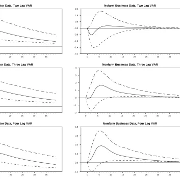
Figures 1 to 3 report the results from our series of robustness checks. These figures each contain six different charts describing the estimated impulse response of hours to a positive technology shock, with each figure using one of three specifications. Figure 1 reports results for the per capita hours specification adopted by CEV. Figure 2 reports results for the first-difference formulation adopted by Gal´ı. Figure 3 reports results using linearly-detrended hours, another specification reported by Gal´ı. The dashed lines on the charts are 10th and
2
90th percentiles from centered bootstrap distributions based on 5000 replications of the estimated reduced-form VAR processes.
The left-hand columns in each of the figures report the results obtained with the data definitions used by CEV. These data are from the US Bureau of Labor Statistics (BLS), with both hours and labor productivity relating to the business sector, which is defined as the aggregate economy excluding the government, household, and non-profit sectors. The right-hand columns report estimates using hours and output for the nonfarm business sector, which also excludes the farm sector. This latter measure of hours is the one used by Gal´ı (1999). In contrast to the results reported here, the output and labor productivity measures employed by Gal´ı relied on total GDP. However, calculations not reported here showed that the use of this measure of output gave essentially the same results as those obtained using nonfarm business output. The measure of population used to construct the per capita hours series is the BLS series on the civilian noninstitutional population aged sixteen and over. All data were downloaded directly from the BLS website during August 2004 and all regressions were run over the sample 1949:Q1 to 2004:Q1.
Per Capita Specification: The bottom-left panel of Figure 1 shows the results from the four-lag per capita specification run on business sector data. This is the specification used by CEV, and our results, which are based on an additional nine quarters of data, essentially replicate their findings: Hours appear to rise on impact and these initial increases are statistically significant according to the bootstrap distribution. Lag selection tests, however, do not favor the four-lag specification: For this specification, and all the others on reported on Figures 1 to 3, the AIC favors three lags, while the BIC favors two lags. Thus, results these additional models are also reported. For the per capita specification, the estimated impact effects of the technology shock on hours from these shorter-lag VARs are still positive, but the 10th percentile estimates are no longer positive, somewhat weakening the evidence in favor of this effect being statistically significant.
serious fragility for results from the per capita specification: Small changes in the definition of output and hours or in the specification of the model’s dynamics, produce economically important changes in the results.
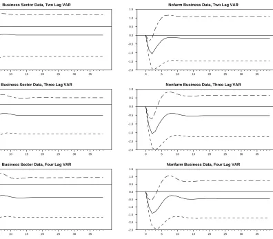
First-Difference Specification: Figure 2 reports the results from the specification fea-turing the log-difference of hours worked. In contrast to the results for the per capita specification, these results show a remarkable similarity across the various data definitions and modelling of dynamics. In each case, the impact effect of a positive technology shock on hours worked is estimated to be negative, and the bootstrapped responses all indicate that this negative response is statistically significant.
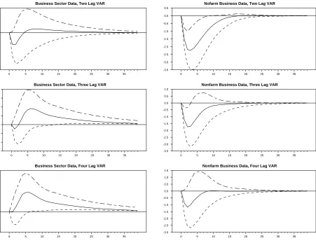
Linear Trend Specification: Figure 3 shows that the results from this specification fall somewhere between the results from the previous two specifications. In each case, the estimated impact effects of a positive technology shock are negative. However, there is not the same uniformity in the pattern of the responses, with the business sector models showing a shallow initial decline (almost zero in the four-lag case) followed by a subsequent increase while the nonfarm business models each show sustained declines. Also, the initial decline only appears to be statistically significant for the two- and three-lag versions of the nonfarm business models preferred by the lag selection tests.
3.2 The Cyclical Importance of Technology Shocks
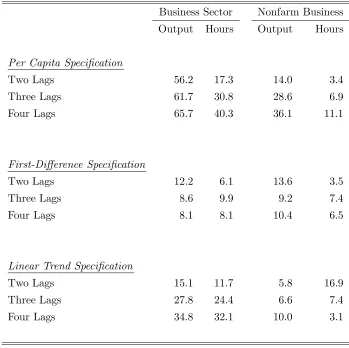
Not surprisingly, the various specifications also differ considerably in their assessment of the role played by technology shocks in determining the cyclicality of output and hours. Table 1 reports the results from performing a set of calculations similar to those in the CEV paper to assess the contribution of technology shocks to the cyclical variance of hours and output per capita.
of a cyclically-adjusted version of the historical series.
The top panel of Table 1 shows how the conclusions obtained from the per capita specification concerning the contribution of technology shocks can be substantially altered by minor changes in data definition (the inclusion or exclusion of the farming sector) and by small changes in the specification of the dynamics. When business sector data are used and the model has four lags, technology shocks are estimated to account for 66 percent of the cyclical variance in output and 40 percent of the cyclical variance in hours. These calculations are similar to the figures of 64 and 33 percent reported by CEV for the same exercise. However, changing the model to use nonfarm business data, these percentages drop to 36 percent for output and 11 percent for hours. And the two-lag version of the nonfarm business model indicates that technology shocks account for only 14 percent of the cyclical variance in output and 3 percent for hours.
In contrast, the results from the first-difference specification tell pretty much the same story, no matter which data set is used or how the dynamics are specified. In each case, the results point to technology shocks playing a very limited role in generating cyclical variation in hours and output. The largest contribution to the variance in output found for this specification is just below 14 percent, while the largest contribution for hours is only 10 percent.
3.3 Accounting for Differences Across Data Sets
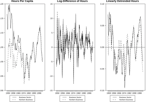
Before discussing the merits of the various specifications in more detail, it is worth exam-ining why the per capita specification’s results are so sensitive to the choice of dataset, while the linear trend specification’s results are less so, and the first-difference approach not at all. Figure 4 displays the three different transformations of hours worked for both the business and nonfarm business sectors. The left panel shows that there is a striking difference between the per capita hours series for the total business and nonfarm sectors during the early part of our sample, up until the early 1970s. Total business hours showed a substantial downward trend over this period that was not evident in the nonfarm sector, as the adoption of modern farming methods led to dramatic reductions in the numbers at work on the land. In light of this chart, it is hardly surprising that the results from this specification are very sensitive to which of these measures is used.
two hours series to behave quite differently for much of the sample, this trend was slow and steady enough for there to be very little difference between the time series for the log-differences. This explains why the results from this specification are robust to the choice of data set.
Finally, the chart helps to explain why the results from the linear trend specification are more stable across datasets than those from the per capita specification, but less so than for those from the log-difference specification. Allowing for separate long-run trends in the two hours series, rather than detrending both with the same population series, allows for the long-running decline in farm hours to be accounted for in the business-sector trend. Thus, the high-frequency movements in these two series track each other better than for the per capita series. However, this also points to a potential problem with the application of this approach to the business sector data: This method still implies separate deterministic trends for business and nonfarm business hours at the end of the sample, even though the left panel shows that farming now accounts for a negligible fraction of hours worked. On balance, then, these considerations point towards the first-difference specification approach as perhaps a more satisfactory approach than the linear detrending method.
4
Assessing the Various Approaches
We have found that the stochastic trend model of hours adopted by Gal´ı produces far more robust results than the per capita hours specification of CEV. On its own, this is an important point in favor of the stochastic trend approach, and thus in favor of its findings that positive technology shocks lead to a decline in hours on impact, and that technology shocks play a limited role in generating the business cycle. However, in addition to the robustness findings, there are other good reasons to favor these results.
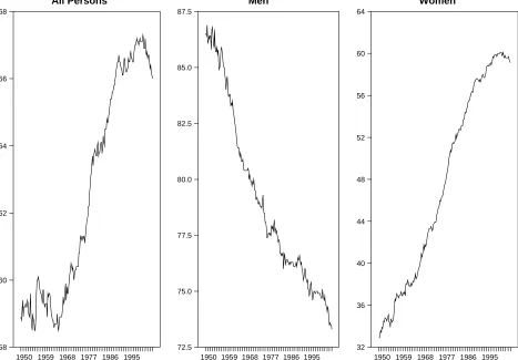
patterns underlying this trend appear to be largely social in nature, with explanations that likely lie outside the realm of the neoclassical growth model: The upward trend in labor force participation has been the result of an almost doubling of participation by women offsetting a slow decline in male participation rates.
These calculations show there are good reasons to believe that there are other forces at work beyond population growth that result in an upward trending nonstationary series for hours worked. However, the difficulty in modelling these trends precisely argues in favor of Gal´ı’s first-difference approach, which views hours as being an I(1) series, but does not take a stance on the exact sources of the stochastic trend underlying the series.3
Second, in relation to the issue of which data series to use, it is widely believed that the nonfarm business measures of output and hours are more accurate than their farm-sector counterparts, and thus that the nonfarm data are more reliable than the business sector data for statistical inference. Data on nonfarm hours are largely based on the large and statistically-precise monthly establishment survey. In contrast, farm hours are mea-sured from the less-reliable household survey. In addition, because of its seasonal nature, farm output is mainly measured on an annual basis, and is thus less comparable with the quarterly measures of nonfarm output.
Finally, there is the issue of the stationarity or nonstationarity of hours per capita. CEV’s paper presented a number of test results to support the argument that their business-sector measure of hours per capita is stationary, and thus appropriate for use in a VAR analysis. However, it is well known to generally be very difficult to use simple statistical tests to make a convincing case either for or against a unit root in the case of persistent series, and a quick glance at the left panel of Figure 4 suggests that the case for stationarity of this series is hardly overwhelming. That said, if one were using purely statistical grounds to motivate one’s choice of model, then a pattern worth noting is that the case for stationarity of the nonfarm hours per capita series is stronger than for business sector series. For example, the Augmented Dickey-Fuller test statistic for per capita nonfarm hours is -3.38, which falls just short of rejecting the unit root hypothesis at the one percent level. In contrast, the ADF statistic for per capita business hours is -2.84, which falls short of the
3
five percent critical value.
These arguments indicate that even if one prefers the per capita specification, there are good reasons to believe that the results for the nonfarm sector are likely to be more reliable than the results for the business sector. And, in this case, both the two- and three-lag models preferred by the lag selection tests point to a negative impact effect on hours of a positive technology shock, and a very limited role for these shocks in generating the business cycle.
5
Conclusions
References
[1] Basu, Susanto, John Fernald, and Miles Kimball (1998). Are Technology Improvements Contractionary?, Federal Reserve Board, International Finance Discussion Paper, 1998-625.
[2] Blanchard, Olivier and Danny Quah (1989). “The Dynamic Effects of Aggregate De-mand and Supply Disturbances,”American Economic Review, 79, 655-673.
[3] Christiano, Lawrence, Martin Eichenbaum and Robert Vigfusson (2003). What Happens After a Technology Shock?, Federal Reserve Board, International Finance Discussion Paper, 2003-768.
[4] Francis, Neville, Michael Owyang and Athena Theodorou (2003). The Use of Long-Run Restrictions for the Identification of Technology Shocks, Federal Reserve Bank of St.
Louis Economic Review, November/December, 53-66.
[5] Gal´ı, Jordi (1999). “Technology, Employment and the Business Cycle: Do Technology Shocks Explain Aggregate Fluctuations,” American Economic Review, 89, 249-271.
[6] Shapiro, Matthew and Mark Watson (1988). “Sources of Business Cycle Fluctuations,”
Table 1: Contribution of Technology Shocks to Cyclical Variance
Business Sector Nonfarm Business Output Hours Output Hours
Per Capita Specification
Two Lags 56.2 17.3 14.0 3.4 Three Lags 61.7 30.8 28.6 6.9 Four Lags 65.7 40.3 36.1 11.1
First-Difference Specification
Two Lags 12.2 6.1 13.6 3.5 Three Lags 8.6 9.9 9.2 7.4 Four Lags 8.1 8.1 10.4 6.5
Linear Trend Specification
Figure 1: Per Capita Specification
Hours Response to Technology Shock (with Bootstrapped 10% and 90% Fractiles)
Business Sector Data, Two Lag VAR
0 5 10 15 20 25 30 35 -1 0 1 2 3 4 5
Business Sector Data, Three Lag VAR
0 5 10 15 20 25 30 35 -1 0 1 2 3 4 5 6
Business Sector Data, Four Lag VAR
2.4 3.2 4.0 4.8 5.6 6.4
Nofarm Business Data, Two Lag VAR
0 5 10 15 20 25 30 35 -3.2 -2.4 -1.6 -0.8 -0.0 0.8 1.6 2.4
Nonfarm Business Data, Three Lag VAR
0 5 10 15 20 25 30 35 -2 -1 0 1 2 3 4
Nonfarm Business Data, Four Lag VAR
Figure 2: First-Difference Specification
Hours Response to Technology Shock (with Bootstrapped 10% and 90% Fractiles)
Business Sector Data, Two Lag VAR
0 5 10 15 20 25 30 35 -2.5 -2.0 -1.5 -1.0 -0.5 0.0 0.5 1.0
Business Sector Data, Three Lag VAR
0 5 10 15 20 25 30 35 -3.0 -2.5 -2.0 -1.5 -1.0 -0.5 0.0 0.5 1.0
Business Sector Data, Four Lag VAR
-2.0 -1.5 -1.0 -0.5 0.0 0.5 1.0
Nofarm Business Data, Two Lag VAR
0 5 10 15 20 25 30 35 -2.0 -1.5 -1.0 -0.5 0.0 0.5 1.0 1.5
Nonfarm Business Data, Three Lag VAR
0 5 10 15 20 25 30 35 -2.5 -2.0 -1.5 -1.0 -0.5 0.0 0.5 1.0
Nonfarm Business Data, Four Lag VAR
Figure 3: Linear Trend Specification
Hours Response to Technology Shock (with Bootstrapped 10% and 90% Fractiles)
Business Sector Data, Two Lag VAR
0 5 10 15 20 25 30 35 -3 -2 -1 0 1 2
Business Sector Data, Three Lag VAR
0 5 10 15 20 25 30 35 -2.4 -1.6 -0.8 -0.0 0.8 1.6 2.4 3.2
Business Sector Data, Four Lag VAR
0 1 2 3 4
Nofarm Business Data, Two Lag VAR
0 5 10 15 20 25 30 35 -3.5 -3.0 -2.5 -2.0 -1.5 -1.0 -0.5 0.0 0.5
Nonfarm Business Data, Three Lag VAR
0 5 10 15 20 25 30 35 -3.5 -3.0 -2.5 -2.0 -1.5 -1.0 -0.5 0.0 0.5 1.0
Nonfarm Business Data, Four Lag VAR
Figure 4: Measures of Labor Input
Hours Per Capita
1950 1958 1966 1974 1982 1990 1998 0.90
0.95 1.00 1.05 1.10 1.15 1.20
Log-Difference of Hours
1950 1958 1966 1974 1982 1990 1998 -15
-10 -5 0 5 10 15
Linearly Detrended Hours
1950 1958 1966 1974 1982 1990 1998 -0.10
Figure 5: Patterns in US Labor Force Participation
All Persons
60 62 64 66 68
Men
75.0 77.5 80.0 82.5 85.0 87.5
Women