Resource-Constrained Project Scheduling
Problem with Flexible Work Proles:
A Genetic Algorithm Approach
M. Ranjbar
1;and F. Kianfar
2Abstract. This paper deals with the resource-constrained project scheduling problem with exible work proles. In this problem, a project contains activities interrelated by nish-start-type precedence constraints with a time lag of zero. In many real-life projects, however, it often occurs that only one renewable bottleneck resource is available and that activities do not have a xed prespecied duration and associated resource requirement, but a total work content, which essentially indicates how much work has to be performed on them. Based on this work content, all feasible work proles have to be specied for the activities, each characterized by a xed duration and a resource requirement prole. The task of the problem is to nd the optimum work prole and start time of each activity in order to minimize the project makespan. We propose a procedure to nd all feasible work proles of each activity and we use a genetic algorithm with a new crossover operator to schedule the activities. Computational results on a randomly generated problem set are presented.
Keywords: Project scheduling; Heuristic; Genetic algorithm.
INTRODUCTION
This research considers the Resource Constrained Project Scheduling Problem with Flexible Work Pro-les (RCPSP FWP). This problem was proposed by Kolisch [1] in the eld of pharmaceutical R&D projects and deals with the lead optimization phase of pharma-ceutical research where a number of leads (molecules as a basis for potential drugs) are processed by dierent departments in order to optimize their biochemical characteristics. The RCPSP FWP can be stated as follows. A single project consists of a set of activities that are interrelated by nish-start-type precedence relations with a time lag of zero. There is a single constrained renewable resource (laboratory) in which all activities have to be processed. For each activity, instead of a xed duration and resource requirement, the total work content is given, which essentially
1. Department of Industrial Engineering, Faculty of Engineer-ing, Ferdowsi University of Mashhad, Mashhad, P.O. Box 91775-1111, Iran.
2. Department of Industrial Engineering, Sharif University of Technology, Tehran, P.O. Box 11155-9414, Iran.
*. Corresponding author. E-mail: m [email protected] Received 8 June 2008; received in revised form 24 January 2009; accepted 8 June 2009
indicates how much work has to be performed. In other words, activity duration and resource usage at each time period of their execution are unknown. The way each activity is processed, i.e. its work prole, is not predetermined but limited by the following ve constraints:
a) No preemption is allowed.
b) The resource usage of each activity in a process-ing period has to be within a resource-dependent interval.
c) The summation over used resource units for all periods of execution of each activity should be equal to the work content of the activity.
d) During processing, the resource usage of each activity has to be constant for a resource-dependent period.
Each work prole for an activity is considered as an activity mode and all feasible work proles for an activity constitute its set of modes.
The constraints (a)-(d) assure that the processing of activities is done in an ecient way by reducing the number of setups due to constraints (a) and (d) and by forbidding the case of too few or to many resources assigned to an activity within one period
by constraint (b). Since the number of feasible work proles of each activity in the general form and on the basis of conditions (a)-(d) may be very large, we limit ourselves to only smooth (SM), Non-Increasing (NI), Non-Decreasing (ND) or triangular (TR) types of gure for work proles. Figures 1 to 4 illustrate some possible work proles of an activity with work content of 15.
The RCPSP FWP is a dierent version of the well-known Resource Constrained Project Scheduling Problem (RCPSP) in which a single renewable resource is available and activity duration and resource usage to a single renewable resource are known constants. Also, the RCPSP FWP is a generalization of the discrete time/resource trade-os (DTRTP), introduced by De Reyck et al. [2]. In the DTRTP, only smooth work
Figure 1. Smooth work prole.
Figure 2. Non-decreasing work prole.
Figure 3. Non-increasing work prole.
Figure 4. Triangular work prole.
proles are considered for each activity, and constraints (b), (c) and (d) are ignored.
To the best of our knowledge, literature on the RCPSP FWP, as dened in this paper, is virtually void. Research eorts have been concentrated on two related problems, RCPSP and DTRTP. Salewski et al. [3], Brucker et al. [4], Kolisch and Padman [5] and Kis [6] include some noteworthy literature survey research for the RCPSP. Also, numerous exact and heuristic procedures are presented in the literature for the RCPSP. Chapter 6 of the project scheduling research handbook of Demeulemeester and Herroe-len [7] gives an extensive literature overview of the RCPSP and, hence it is not repeated here. In addi-tion, Kolisch and Hartmann [8] present a classication and performance evaluation of dierent heuristic and metaheuristic algorithms for the RCPSP. De Reyck et al. [2] present several heuristic procedures for the DTRTP based on the Tabu Search (TS) and some local searches. These heuristic procedures are based on the decomposition of the problem into a mode assignment phase and a resource-constrained project scheduling phase with xed mode assignments. De-meulemeester et al. [9] have developed a Branch-and-Bound algorithm (B&B) for the DTRTP based on the concept of activity-mode combinations, i.e. subsets of activities executed in a specic mode. Also, Ranjbar et al. [10] present an ecient hybrid meta-heuristic, based on the scatter search for the DTRTP and RCPSP.
The NP -hardness of the RCPSP was shown by Blazewicz et al. [11] as a generalization of the job shop scheduling problem. Furthermore, Demeulemeester et al. [9] show that the DTRTP, as a generalization of the parallel machine problem, is strongly NP -hard. Therefore, the RCPSP-FWP as a generalization of the DTRTP is strongly NP -hard.
Since the RCPSP FWP is a very complex prob-lem, we use a Genetic Algorithm (GA) as our solu-tion approach. Two famous GAs applied to project scheduling problems are Mori and Tseng [12] and Hartmann [13].
The contribution of this paper is twofold. First, we present a linear model for the RCPSP FWP and also an enumeration scheme to generate feasible work proles. Second, we propose a metaheuristic solution procedure based on GA to solve RCPSP FWP.
The outline of the paper is as follows. First, the problem formulation and notation are described and generation of feasible work proles of a single activity is discussed. After that, schedule representation and the generation scheme are explained and the general structure of the genetic algorithms and its operators are described. In the section following these computational results are reported. Finally, overall conclusions and suggestions for future research are drawn.
PROBLEM FORMULATION AND NOTATION
The objective of the RCPSP FWP is to schedule each activity of a project in one of its dened modes subject to precedence and resource constraints, in order to minimize the project makespan. The parameters used are dened in Table 1.
The dummy activities, 0 and n + 1, represent the start and completion of the project, respectively, with wo= wn+1= 0. The RCPSP FWP can be formulated
by introducing the following decision variables: sit=
(
1; if activity i is started at time instant t 0; otherwise
fit=
(
1; if activity i is nished at time instant t 0; otherwise
hit=
(
1; if ri(t 1)6= ri(t)
0; otherwise
In the following, we represent an MIP formulation for the RCPSP FWP.
min Z =
lfXn+1 t=efn+1
tf(n+1)t; (1)
subject to:
lsi
X
t=esi
sit= 1; i 2 N; (2)
lfi
X
t=efi
fit= 1; i 2 N; (3)
Table 1. Notation.
N = f0; ; n; n + 1g Set of activities with index i E = f(i; j); i; j 2 Ng Set of precedence relations
Pi Set of all predecessors of activity i; i 2 N
Si Set of all successors of activity i; i 2 N
a Constant availability of the single renewable resource wi Work content of activity i; i 2 N
ri; ri Lower and upper bounds of resource usage of activity i in each
time period; i 2 N
t Minimum number of consecutive periods where all activities should have a constant resource usage
di Duration of activity i; i 2 N
di=
l
wi
ri
m
Lower bound for duration of activity i; i 2 N
di=
j
wi
ri
k
Upper bound for duration of activity i; i 2 N dmin
i Minimum possible duration for a feasible work prole of
activity i; i 2 N d0min
i Minimum possible duration for an infeasible work prole of
activity i with minimum violation; i 2 N T =Pn
i=1di An upper bound on the project makespan
esi= max
( P
j2Piwj
a
!
; maxj2Pi
esj+ dminj
)
Earliest start time of activity i; i 2 N efi= esi+ di Earliest nish time of activity i; i 2 N
lfi= min
( T
P
j2Siwj
a
!
; (T minj2Siflsjg)
)
Latest nish time of activity i; i 2 N lsi= lfi di Latest start time of activity i; i 2 N
(t) = (t 1; t] Time period (t); t = 1; 2; ; T
ri(t) Resource usage of activity i at time period t; i 2 N,
t = esi+ 1; ; lfi
lfi
X
t=esi+1
ri(t)= wi; i 2 N; (4)
lfi
X
t=efi
tfit lsj
X
t=esj
tsjt; 8(i; j) 2 E; (5)
n
X
i=1
ri(t) a; t = 1; ; T; (6)
ri(0)= 0; i 2 N; (7)
t+t 1X =t
hi 1; i 2 N; t = esi+ 1; ; lfi; (8)
ri(t+1) ri(ri(t)+ sit); i 2 N; t = 1; ; T; (9)
ri(t) ri(ri(t+1)+ fit); i 2 N; t = 1; ; T; (10)
ri(t+1) ri(t) ri:hi;t+1; i 2 N; t = 1; ; T; (11)
ri(t) ri(t+1) ri:hi;t+1; i 2 N; t = 1; ; T; (12)
sit; fit; hit2 f0; 1g; i 2 N; t = 1; ; T; (13)
ri(t)2 f0g [ fri; ri+ 1; ; rig;
i 2 N; t = 1; ; T: (14)
Objective Function 1 minimizes the project makespan. Constraints 2 and 3 ensure that exactly one start and nish time are assigned to each activity, respectively. Constraint 4 assures that used resource units by each activity are equal to the activity work content. Con-straints 5 and 6 indicate the precedence and resource constraints, respectively. Constraint 7 indicates that the resource is available after time instant zero. Con-straint 8 corresponds to the conCon-straints (d) of the work prole constraints. Also, Constraints 9-12 ensure that every change in the level of resource usage for each activity is less than its resource usage upper bound. Finally, Constraints 13 and 14 show the value domains of the decision variables.
ASSIGNMENT OF FLEXIBLE WORK PROFILES
In this section, we consider the problem of generating feasible work proles of a single activity within the RCPSP FWP. We rst propose a model that generates the work prole with minimum durations. Next, we present an enumeration procedure for generating the NI, ND and SM work proles. We further discuss the generation of TR work proles based on NI and ND work proles.
Generation of Work Proles with Minimum Duration
Based on the dened notations in Table 1 and the denition of the two following decision variables, we present a model for nding a feasible work prole with minimum duration for each single activity, i 2 N.
xri= number of periods with a resource usage of
r units during execution of activity i 2 N(r = ri; ri+ 1; ; ri);
yri=
8 > > > < > > > :
1; if there is at least one period with resource usage of r units during execution of activity i
0; otherwise
dmin
i = min
ri
X
r=ri
xri; (15)
subject to:
ri
X
r=ri
rxri= wi; (16)
tyri xri diyri; (17)
xri2 f0; 1; g; r 2 [ri; ri]; (18)
yri2 f0; 1g; r 2 [ri; ri]: (19)
Objective Function 15 minimizes the number of periods where the activity has a positive resource usage and, thus the duration of the activity. Constraint 16 takes care that the total used resource units equals the activity work content. Constraint 17 couple xri
-variable with the yri-variable; if yri= 0, then xriis set
to zero, otherwise, if yri = 1, t xri di. Finally,
Constraints 18 and 19 show the value domains of the decision variables. We call Constraints 16 to 19 the Feasible Work Prole Space (FWPSi) for activity i. If
FWPSi = ;, there is not any feasible work prole for
activity i. In this case, we consider the work proles with minimum violation.
Generation of Work Proles with Minimum Violation
In the case there is no feasible work prole for an activity, we consider only one work prole for the activity which has a minimum violation from work prole constraints. To this purpose, we alter the previous model in order to nd an infeasible work
prole that minimizes the number of periods that are short of the minimum number of periods with constant duration t. We dene decision variable vri 0 as the
number of periods with resource usage r short of the minimum number of periods regarding to activity i. Note that vriis formally dened as vri= max(0; t xri)
and the new model is as follows: d0min
i = min
ri
X
r=ri
vri; (20)
subject to:
ri
X
r=ri
rxri= wi; (21)
tyri vri xri diyri; r 2 [ri; ri]; (22)
xri2 f0; 1; g; r 2 [ri; ri]; (23)
yri2 f0; 1g; r 2 [ri; ri]; (24)
vri 0; r 2 [ri; ri]: (25)
Objective Function 20 minimizes the number of periods that are short of the minimum number of periods with a constant resource usage. Altered Constraint 22 sets the variable, vri. Other constraints are taken from the
previous model.
An Enumeration Procedure for the ND Work Proles
In order to enumerate all ND work proles of an activity, i, we use an enumeration tree in which level l(l = 1; ; ri ri+1) corresponds to all possible values
of xri, dened as the number of periods with a resource
usage of r = l 1 + ri units. In each node of level l, ^wi
indicates the remaining work content of activity i, i.e. the work content of activity i minus the total assigned resource units in nodes located on the path from the start node (l = 0) to the current node. At each level, l > 0, there are t t + 1 possible descendants for a parent node, located at level l 1 where t = b ^wi=rc.
These descendants are generated by assigning dierent values to xrifrom set f0; t; t+1; ; tg. The remaining
work content is updated as ^wi := ^wi rxri after
assignment. We dene a block in a work prole as a number of consecutive periods with equal levels of resource usage and xi = (xri; xri+1; ; xri) as the
block representation of the work prole of activity i in which xr represents the length of the block with a
resource usage of r units where r 2 [ri; ri]. In each
node of the enumeration tree wherein we face one of the following conditions, we fathom the node.
1. Finding a feasible work prole, i.e. ^wi = 0. In
this case, the feasible work prole is obtained by following the path between the start node and the current node.
2. Finding a positive remaining work content that is not enough for the extension of more blocks, i.e. in a level, l = r + 1 ri, 0 < ^wi< t(r + 1).
3. Reaching an infeasible work prole. If in each node of level l = r + 1 ri we replace ^wi with wi and
ri with r in the model for FWPSi, and we nd
FWPSi = ;, then all descendants of this node will
be infeasible.
4. Reaching the last level of the enumeration tree, i.e. l = ri ri+ 1.
To generate all NI work proles, we correspond each NI work prole xi = (xri; xri+1; ; xri) to the
ND work prole x = (xri; xri 1; xri).
Generation and Enumeration of the TR Work Proles
All feasible TR work proles of each activity can be generated from its ND or NI work proles. It should be noted that ND and NI work proles are two special types of TR work prole. Also, SM work proles are an especial type of ND and NI work proles. Thus, we can conclude SMNITR and SMNDTR. Each ND work prole has a unique corresponding NI work prole and possibly some other TR work proles constituting a set called a neighborhood. To generate all feasible TR neighbors of a feasible ND work prole, we do as follows. Assume the feasible ND work prole includes b dierent resource usage levels, as x = (xr1; xr2; ; xrb), where r r1 < r2 < < rb r
and block rb is the vertex of each generated TR work
prole. We may use block rb for 1 b < b in both left
and right legs of each generated TR work prole with durations xl
rb and xrrb, respectively. If the duration of
a single block, rb, is xrb 2t, we can distribute xrb
between xl
rb and xrrb. The number of dierent ways of
this work is equal to the number of common solutions of the following equations:
xl
rb+ xrrb= xrb; (26)
xl rb; x
r
rb2 f0; t; ; xrbg: (27)
If xrb 2t, the number of solutions of Equations 26
and 27 is equal to xrb 2t + 3, including:
f(xl
rb = 0; xrrb= xrb); (xlrb= t; xrrb= xrb t);
(xl
rb = t + 1; x r
rb = xrb t 1); ;
(xl
and, if xrb < 2t; we will have only two possible values
for xl
rb and xrrb, i.e.:
f(xl
rb= xrb; xlrb = 0); (x l rb = 0; x
l
rb= xrb)g:
If we dene function f for integer numbers as: f(a) =
(
a; a 0
1; a < 0
we generally have f(xrb 2t) + 3 dierent solutions
for Equations 26 and 27. Thus, the number of total dierent feasible TR work proles that can be obtained from a feasible ND work prole, x = (xr1; xr2; ; xrb),
is equal toQb 1b=1(f(xrb 2t) + 3).
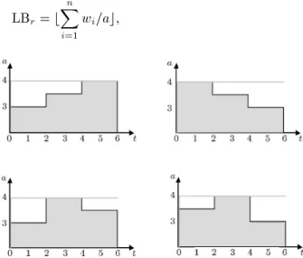
It can be seen that the FWPS for each activity is constituted of dierent neighborhoods. At the core of each neighborhood, there are two feasible work proles, NI and ND, and other neighbors are possibly other feasible TR work proles. Each feasible TR work prole can be obtained from only one core and, hence, is located in only one neighborhood. Therefore, FWPS is partitioned by this neighborhood denition. Figure 5 shows one ND, one NI and two TR work proles that constitute a neighborhood.
Upper and Lower Bounds of the Project Makespan
Regarding Equations 15 to 19, we obtain the up-per bound UB for the project makespan as UB= Pn
i=1dmini . The project makespan lower bound LB is
the maximization of a critical path-based lower bound LB0 and a resource-based lower bound LBr. The
lower bound LB0is obtained by calculating the critical
path in the activity network, where each activity, i, is assigned its shortest feasible work prole with duration dmin
i , taking into account the resource availability, a.
The resource-based lower bound LBr is computed as:
LBr= b n
X
i=1
wi=ac;
Figure 5. An example of four neighbor work proles.
where bxcdenotes the largest integer equal to, or less than, x.
SCHEDULE REPRESENTATION AND GENERATION SCHEME
Our constructive heuristic algorithm uses a schedule representation to encode a project schedule and a Schedule Generation Scheme (SGS) to translate the schedule representation to a real schedule. The SGS determines how a feasible schedule is constructed by assigning starting times to the activities whereby the relative priority and activity work proles are deter-mined by the schedule representation in our algorithm. There are various approaches for both the representa-tion and generarepresenta-tion of a schedule.
We represent a schedule, S, of the RCPSP FWP by a double list (; wp). The rst list is a vector, = (1; ; n), such that positive real number i 2 R+
represents the priority value of activity i. This list was introduced by Kolisch and Hartmann [14] as Random Key (RK) representation for the RCPSP. The second list is a work prole list wp = (wp1; ; wpn) where
wpi represents the work prole chosen for activity i.
We utilize a modied version of the RK representation developed by Debels et al. [4] in which the Topological Order (TO) concept is used in the construction of the RK, which we denote as TORK. Each TORK is constructed by scheduling the activities using a SGS, obtaining schedule S and considering priority values as i= si(S); 8i 2 N where si(S) indicates the start time
of activity i in schedule S. For a detailed discussion of the advantages of the topological order representation, we refer to [15].
Besides dierent schedule representations, there also exist three dierent types of SGSs in the literature: the Serial SGS (SSGS), the parallel SGS and the bidirectional SGS [16]. As it is sometimes impossible to reach an optimal solution with parallel and bidirec-tional SGSs, we opt for serial SGS. At each iteration of the SSGS, the activity with the highest priority is chosen and assigned the rst possible starting time such that no precedence or resource constraint is violated. Although any generated schedule of the RCPSP by the SSGS belongs to the set of active schedules [17], it does not necessarily hold for the RCPSP FWP.
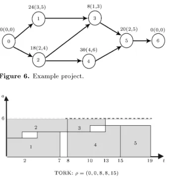
Figure 6 illustrates an example project with ve non-dummy activities and one renewable resource with a = 6 and t = 2. The schedule of Figure 7 is obtained, based on the random priority list, = (1; 2; 3; 4; 5), and SSGS. The corresponding TORK is = (0; 0; 8; 8; 15). GENETIC ALGORITHM
We propose a genetic algorithm to schedule activities in a RCPSP FWP. The general structure of our GA
Figure 6. Example project.
Figure 7. A schedule and its TORK.
Figure 8. General structure of GA.
is shown in Figure 8. The procedure starts with the random generation of an initial population, P , with size of psize of schedules. In order to generate each element, e = (; wp), of initial population, P , we generate a random priority list, , randomly select a work prole for each activity from its set of feasible work proles and decode element, e, to a real schedule using SSGS. Then, the procedure is followed by an iterative process that continues until the termination criterion is satised. The iterative process consecutively applies crossover, mutation and local search operators in order to generate new solutions with higher quality. In the second step, the NewP , representing a new population, is initialized as an
empty set and will include the generated schedules in each iteration. In order to construct the new elements, each element, e = 1; ; psize of P , considered as the father schedule (Sf), is mated randomly with element
c (c 6= e and 1 c psize) of P , considered as the mother schedule (Sm), to constitute a couple. Each
couple generates two children schedules considered as the son schedule (Ss) and the daughter schedule (Sd).
The children generation process is performed using two operators, i.e. crossover and mutation where mutation is applied with probability pmut. The child with the
better makespan obtained using SSGS is chosen as the selected child schedule (Sc). To improve Sc, a local
search procedure is applied to it with probability pls.
Then, P is updated by transferring all elements of NewP to it.
Crossover
After the selection of parents, a crossover operation combines the Sf and Sm to generate Ss and Sd. We
use a two-point crossover operator, based on the idea of replacement of weak schedules with better sub-schedules, in which the crossover points are determined, based on the resource prole for the given schedule. The crossover point, cp1, is dened as an activity's start
time and the crossover point, cp2, is dened as an
activ-ity's nish time. All activities executed totally between these two crossover points are called a sub-schedule. We dene the Resource Utilization Ratio (RUR) as follows. Let A[t1; t2] = fijsi t1 and fi t2g as the
set of activities that are executed totally in interval [t1; t2]. The RUR for schedule S in interval [t1; t2] is
dened as RURS[t
1; t2] = Ptt=t2 1+1
P
i2A[t1;t2](rit=a).
In order to determine crossover points, we look for sub-schedules including at least bn=3c and, at most, d2n=3e activities giving the maximum RUR. Assume cp1= si
and cp2 = fj, where i; j 2 f1; ; ng and subject to
the two following conditions: I) sj si,
II) fj> fi or fj= fi where j 6= i.
For all real activities i and j, we consider all possible intervals bt1 = si; t2 = fjc regarding Conditions I and
II as the candidates for the cross points. The two points, t
1and t2, are considered as the crossover points,
cp1 and cp2, respectively, for which the maximum
resource utilization ratio is obtained. In other words, the cross points are determined based on the following condition:
RURS[t
1; t2] RURS[t1; t2];
8t1= si;
t2= fj; i; j = 1; ; n;
and holding Conditions I and II.
Each activity, i, for which si cp1 and fi cp2,
constitutes the subset Nsub. In the following, we
describe how the son schedule, Ss, is built from Sf and
Sm. First, we determine cp1(Sf) and cp2(Sf) using
the above mentioned two-point crossover operator. To generate the vectors, s and Xs, of the Ss, for every
activity, i 2 N, we dene the following combination rule. If in schedule Sf activity i 2 Nsub, let si = fi
and wpsi = wpfi. Otherwise, if fi < cp1(Sf), let
si= mi b and wpsi = wpmi and if fi > cp1(Sf),
let si = mi+ b and wpsi = wpmi where b is a very
big constant.
This combination rule allows the crossover op-erator to place the good sub-schedules with the high resource utilization of the Sf in Ss and replace the
weaker sub-schedules of the Sf with the lower resource
utilization by corresponding sub-schedules of the Sm.
The big constant b is used in order to prevent the relative priority structure between the activities of a case being mixed with the priority values of activities of another case in the combination rule. By applying a SSGS on the obtained s and wps, Ss is obtained.
If we assume Sc = Ss, by obtaining the TORK
corresponding to Sc and applying the SSGS to it, the
generation of Sc is nished. By exchanging the role of
Sf and Sm in generation of the child schedule, Sd can
be easily obtained. Based on the lower makespan, Ss
or Sd is selected as the child schedule, Sc. Schedules
represented in Figures 9 to 11 are related to the ex-ample network of Figure 6 and illustrate the crossover operator in which son schedule Ssis considered as the
selected child schedule Sc.
Figure 9. Father schedule (Sf).
Figure 10. Mother schedule (Sm).
Figure 11. Child schedule (Sc).
Mutation
After applying the crossover operator, each generated schedule is muted with a probability of pmut using
a mutation operator that works as follows. First, it selects, randomly, nrm out of n non-dummy activities as the chosen activities for mutation. Then, for each selected activity i, it chooses, randomly, a feasible work prole from the non-neighbors work proles of its current work prole, wpi. Finally, for the selected
activity i, it changes the priority value as i= i+ ri,
where ri2 [1=3f; 2=3f] is a random integer.
Local Search
A local search procedure is applied over each generated schedule with probability Pls, described by a
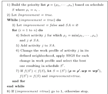
Pseudo-code in Figure 12. In this procedure, given a schedule S, f(S) denote the makespan of schedule S, Improve-ment is a Boolean variable and SA indicates the set of selected activities for a change in the work prole. This procedure tries to decrease f(S) by alternating the work prole of each activity in the neighborhood of the activity work prole.
This procedure includes a While loop, in which all activities are selected based on their priority values,
spectively. In the main step (Step 6) of this procedure, for each selected activity j, all neighbors of its current work prole are replaced one by one as the work prole of activity j, while the other activities' work proles and priority values are not changed. Each generated schedule in Step 6 is evaluated using its makespan and, nally, the best work prole is selected for activity j, resulting in schedule S0. If f(S0) < f(S), schedule S0is
replaced with schedule S and Improvement is changed to true. In the last step, the procedure is stopped if no improvement is obtained; otherwise, it goes to the rst step and updates the priority values based on the best found schedule of the loop.
COMPUTATIONAL RESULTS Benchmark Problem Set
We have coded the procedure in Visual C++ 6.0 and performed all computational experiments on a PC Pentium IV 3GHz processor with 1024 MB of internal memory. We have validated the procedure on two sets of instances developed by Kolisch [1]; one with 30 non-dummy activities and one with 60 non-dummy activities (additionally, each instance has a dummy start and a dummy end activity, each with a duration of zero and a work content of zero). These instances have been generated by transforming a subset of instances from the 30- and 60-activity sets of the instances as available in the PSPLIB library (http://www.bwl.uni-kiel.de/bwlinstitute/Prod/psplib/datasm.htm. Only one renewable resource is considered in the generation of these instances.
Each instance is characterized by the following four parameters: rurf, t min, rsf and NC, which are detailed below.
a) rurf stands for the resource usage range factor. It determines for each activity i the range of [ri; ri]
for the per period resource usage of this activity. rurf 2 [0; 1] where 0 denes a range with ri = ri
and 1 denes a large range. In these two sets of instances, rurf is set to 0.1 and 0.3, respectively. Based on the rurf value, for each activity i, ri and ri are calculated as ri = bwi(1 rurf)c and ri =
dwi(1 + rurf)e.
b) t min stands for the minimum number of consecu-tive periods where activity i has to have a constant resource usage. t min has been set to 1 and 3 for all activities, respectively.
c) rsf stands for the resource strength factor. rsf determines the scarcity of the resources. For rsf = 0, the resources will be as scarce as possible to allow a feasible solution. For rsf = 1, the amount of capacity is such that the resource constraints are
not binding any more. In our problem instance, rsf has been set to 0.2 and 0.5, respectively.
d) NC stands for the network complexity. It measures the average number of non-redundant arcs per activity in the network. NC has been set to 1.5, 1.8 and 2.1, respectively.
Using a full factorial design, 2223 = 24 instances
have been generated with 30 and with 60 activities, respectively. Also, for each activity i, the work content, wi, is a random integer from interval [1; 100].
Parameter Settings
To test our procedure, we predene the settings of the parameters of the genetic algorithm. The number of children, nrc, is xed at 2, the number of mutated activities in the mutation step is set equal to n=10. Using ne tuning, we obtained the values of pmut and
pls parameters as pmut = 0:04, pls = 0:1. Also, the
ned tuned values of psize related to the stop condition are considered as three CPU-time-limits 1, 10 and 50 seconds, and the size of the problem-instances are shown in Table 2.
Number of Feasible Work Proles
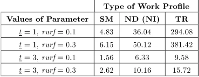
Table 3 indicates the average number of feasible NI, ND and TR work proles for each activity based on the dierent values of parameters t and rurf. It can be seen that the number of feasible work proles is an increasing function of 1=t and rurf.
Detailed Computational Results
The performance of the GA for the RCPSP FWP on the 24 instances is summarized in Table 4. We report the total sum of the makespan of each obtained solution
Table 2. Tuned values of psize. Instances CPU-Time-Limit (s)
Set 1 10 50 J30 50 110 425 J60 30 75 400
Table 3. Average number of feasible work proles. Type of Work Prole Values of Parameter SM ND (NI) TR t = 1, rurf = 0:1 4.83 36.04 294.08 t = 1, rurf = 0:3 6.15 50.12 381.42 t = 3, rurf = 0:1 1.56 6.33 9.58 t = 3, rurf = 0:3 2.62 10.16 15.72
Table 4. Detailed computational results.
Problem Set CPU-Time Limit (s) Data Set J30 J60 5 1410 2310 Sum of the makespans 10 1319 2221 50 1027 1783 5 35.03% 38.61% Average deviation from the LB 10 32.74% 37.11% 50 25.49% 29.75%
and the average deviation from the lower bound LB, described previously.
Table 5 shows the eect of the work prole types. The results are presented as the average deviation from the LB for 1, 10 and 50 seconds CPU-time-limit and for four types of work prole: SM, ND, NI and TR. The results related to TR and SM work prole are the best and the worst, respectively. This result is in line with our expectations because SMNITR and SMNDTR.
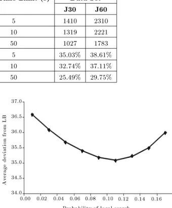
Impact of the Mutation and the Local Search Figures 13 and 14 indicate the impact of the mutation and the local search on the RCPSP FWP results by changing pmut and pls, respectively. The results are
obtained based on the average percent deviation from
Table 5. Eect of the work prole types. CPU-Time Limit (s) Work Prole 5 10 50 SM 44.16% 42.87% 41.59% ND 37.64% 36.28% 29.47% NI 37.69% 36.27% 29.45% TR 35.22% 35.06% 26.48%
Figure 13. Impact of the mutation operator.
Figure 14. Impact of the local search operator.
the lower bound LB when the allowed CPU-time limit is 10 seconds. The results reveal that the best values for the probability of applying these two operators on each generated schedule are as pmut= 0:04 and pls= 0:1.
CONCLUSION
In this paper, we introduced the Resource-Constrained Project Scheduling Problem with a Flexible Work Pro-le (RCPSP FWP). We developed a linear model for the problem, an enumeration procedure for generation of feasible work proles and a metaheuristic, based on the Genetic Algorithm (GA), for solving the problem. As the crossover operator, the GA uses a two-point crossover based on the idea of the replacement of weak sub-schedules with better ones. To that purpose, we used the resource utilization ratio to evaluate dierent sub-schedules. We also developed a local search in-corporated with GA to improve the solutions' quality. We performed detailed computational results on two problem sets, J30 and J60, each including 24 problem instances.
Our future research eorts will focus on two extensions. First, we focus on developing an exact solution approach for the RCPSP FWP and also better metaheuristics. Second, we focus on considering work proles in general forms and developing a procedure to generate them.
REFERENCES
1. Kolisch, R. \Selection and scheduling of pharmaceuti-cal research projects", Perspectives in Modern Project Scheduling, Chapter 13, Springer-Verlag (2006). 2. De Reyck, B., Demeulemeester, E. and Herroelen, W.
\Local search methods for the discrete time/resource trade-o problem in project networks", Naval Research Logistic Quarterly, 45, pp. 553-578 (1998).
3. Salewski, F., Schirmer, A. and Drexl, A. \Project scheduling under resource and mode identity: model, complexity, methods, and application", European Journal of Operational Research, 72, pp. 88-110 (1997).
4. Brucker, P., Drexl, A., Mohring, R., Neumann, K. and Pesch, E. \Resource-constrained project scheduling: notation, classication, models and methods", Euro-pean Journal of Operational Research, 112, pp. 3-41 (1999).
5. Kolisch, R. and Padman, R. \An integrated survey of deterministic project scheduling", Omega, 29, pp. 249-272 (2001).
6. Kis, T. \Project scheduling: A review of recent books", Operations Research Letters, 33, pp. 105-110 (2005). 7. Demeulemeester, E. and Herroelen, W., Project
Scheduling: A Research Handbook, Kluwer Academic Publishers (2002).
8. Kolisch, R. and Hartmann, S. \Experimental inves-tigation of Heuristics for resource-constrained project scheduling: an update", European Journal of Opera-tional Research, 174, pp. 23-37 (2006).
9. Demeulemeester, E., De Reyck, B. and Herroelen, W. \The discrete time/resource trade-o problem in project networks: A branch and bound approach", IIE Transaction, 32, pp. 1059-1069 (2000).
10. Ranjbar, M., De Reyck, B. and Kianfar, F. \A hybrid scatter search for the discrete time/resource trade-o problem in project scheduling", European Journal of Operational Research, 100, pp. 35-48 (2009).
11. Blazewicz, J., Lenstra, J.K. and Rinnooy Kan, A.H.G. \Scheduling subject to resource constraints: classica-tion and complexity", Discrete Applied Mathematics, 5, pp. 11-24 (1983).
12. Mori, M. and Tseng, C.C. \A genetic algorithm for multi-mode resource-constrained project scheduling problem", European Journal of Operational Research, 100, pp. 134-141 (1997).
13. Hartmann, S. \Project scheduling with multiple modes: A genetic algorithm", Annals of Operations Research, 102, pp. 111-135 (2001).
14. Kolisch, R. and Hartmann, S. \Heuristic algorithms for solving the resource-constrained project scheduling problem: classication and computational analysis", in Project Scheduling-Recent Models, Algorithms and Applications, Weglarz, J., Eds., Kluwer Academic Publishers, Boston, pp. 147-178 (1999).
15. Debels, D., De Reyck, B., Leus, R. and Vanhoucke, M. \A hybrid scatter search/electromagnetism meta-heuristic for project scheduling", European Journal of Operational Research, 169, pp. 638-653 (2006). 16. Klein, R. \Bidirectional planning: Improving
prior-ity rule-based heuristics for scheduling resource con-strained projects", European Journal of Operational Research, 127, pp. 619-638 (2000).
17. Kolisch, R. \Serial and parallel resource-constrained project scheduling methods revisited: theory and com-putation", European Journal of Operational Research, 43, pp. 23-40 (1996).
BIOGRAPHIES
Mohammad Ranjbar was born on January 9th, 1978 in Mashad, Iran. He obtained his BS and PhD from the Department of Industrial Engineering at Sharif University of Technology in 2000 and 2007, respectively, receiving his MS from the Faculty of Engineering at Tehran University. From October 2005 to March 2006, he was a visiting PhD student at the Department of Operations Management of the London Business School. In February 2008, he joined Ferdowsi University in Mashhad and, presently, is assistant professor of Industrial Engineering at this university. Dr. Ranjbar is the author of six papers published in international journals, one of which was presented at an international conference.
Ferydoon Kianfar was born on May 17th, 1942 in Tehran, Iran, later receiving his BS in Mechanical Engineering from Tehran Polytechnic. He obtained his MS and PhD in Industrial Engineering from Illinois Institute of Technology (IIT) in Chicago, USA, where, from 1969 to 1970, he was employed as an assistant professor. Since 1970 he has been working at Sharif University of Technology in Tehran, Iran, and is now a full professor of Industrial Engineering.