Sharif University of Technology
Scientia IranicaTransactions E: Industrial Engineering www.scientiairanica.com
Solving a discrete congested multi-objective location
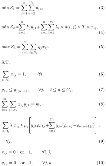
problem by hybrid simulated annealing with customers'
perspective
M. Ghobadi
a, M. Seifbarghy
a, R. Tavakoli-Moghadam
band D. Pishva
c; a. Faculty of Engineering, Alzahra University, Tehran, Iran.b. Faculty of Industrial Engineering, University of Tehran, Tehran, Iran.
c. Faculty of Asia Pacic Studies, Ritsumeikan Asia Pacic University, Beppu, Japan. Received 29 January 2014; received in revised form 1 October 2014; accepted 22 August 2015
KEYWORDS Location-allocation; Queuing;
Modeling; Optimization; VNS;
SA;
Multi-objective.
Abstract. In the current competitive market, obtaining a greater share of the market
requires consideration of the customers' preferences and meticulous demands. This study addresses this issue with a queuing model that uses multi-objective set covering constraints. It considers facilities as potential locations with the objective of covering all customers with a minimum number of facilities. The model is designed based on the assumption that customers can meet their needs by a single facility. It also considers three objective functions, namely minimizing the total number of the assigned server, minimizing the total transportation and facility deployment costs, and maximizing the quality of service from the customers' point of view. The main constraint is that every center should have less than b numbers of people in line with a probability of at least upon the arrival of a new customer. The feasibility of the approach is demonstrated by several examples which are designed and optimized by a proposed hybrid Simulated Annealing (SA) algorithm to evaluate the model's validity. Finally, the study compares the performance of the proposed algorithm with that of Variable Neighborhood Search (VNS) algorithm and concludes that it can arrive at an optimal solution in much less time than the VNS algorithm.
© 2016 Sharif University of Technology. All rights reserved.
1. Introduction
In recent years, due to the growing demand to reduce the transportation costs, attempts to model and opti-mize locations of commercial facilities have signicantly increased. In general, these types of modeling are called location-allocation modeling. Location-allocation is about nding the best possible sites for one or more facilities by examining their relationship and associated *. Corresponding author. Tel.: +81 0977 78 1261;
Fax: +81 0977 78 1261
E-mail addresses: [email protected] (M. Ghobadi); [email protected] (M. Seifbarghy);
[email protected] (R. Tavakoli Moghadam); [email protected] (D. Pishva)
constraints with existing and potential centers with the intention of optimizing them for a specic purpose. The optimization objective can be transportation cost reduction, providing fair services to the clients, gaining a greater share of the market, and so on. In location-allocation models, in addition to selecting the right places for facilities, careful consideration of customer demands and preferences can be a step forwards for the facilities' growth. Some important factors to consider are travel time and waiting time. Oftentimes, cus-tomers are quite annoyed when they are kept waiting for a long time for the service. This paper employs queuing techniques to review and optimize such factors in the modeling process. Considering that optimal location-allocation has to deal with many factors, the
approach has been categorized based on issues it needs to deal with. Many studies have been carried out in the eld and this section highlights some of the major ones.
A Set Covering Problem (SCP), which was rst developed by Toregas et al. (1971), is one of the initial studies that aims to minimize the cost for a group of customers who receive services from multiple facil-ities [1]. Shanthikumar and Yao (1978) investigated server allocation models for the manufacturing site using a pre-dened queuing network that showed the location of work centers [2]. Hakimi (1983) introduced the competitive location model which followed the proximity rule in a network [3]. Revelle and Hogan (1988) proposed Probabilistic Location Set Covering Problem (PLSCP), which ensured that all demands were covered within a predetermined reliability [4]. Marianov and Revelle (1994) developed the PLSCP and proposed Queuing PLSCP (Q-PLSCP), which modeled each facility as a multi-server queuing system and optimized the waiting time by using server utiliza-tion ratio [5].
Marianov et al. (1999) studied the location prob-lem in a competitive environment [6]. Marianov and Serra (2000) investigated the hierarchical location problem in a congested environment where all cus-tomers were initially referred to as a low-level server and elevated to a higher-level server on a need basis [7]. Marianov and Serra (2002) proposed a multi-server set covering problem with restriction on waiting time, wherein every center was restricted in such a way that probability of existing b people in line upon arrival of a new customer could not be greater than [8]. Shavandi and Mahlooji (2006) proposed a new mathematical model for location-allocation of emergency facilities such as hospitals, re stations, and so on, by utilizing queue and fuzzy theory in the model [9]. Rajagopalan and Saydam (2009) proposed a new model for optimal location of ambulances with the objective of minimizing the travel distance while ensuring service support. Their approach utilizes hypercube queuing models to determine the probability of engaging any server and tabu search algorithm for maximizing the coverage [10]. Restrepo et al. (2009) extended the ambulance location modeling to an emergency system with the objective of allocating a certain number of ambulances to a set of sites in such a way that percentage of missing demand was minimized within a standard time limit [11].
Liu and Xu (2011) investigated a location-allocation problem in a fuzzy and random combina-torial environment, wherein a customer demand was expressed by a random combinatorial variable and transportation cost assumed by a fuzzy variable. They also proposed an integer linear programming model with genetic algorithm to solve the fuzzy location-allocation problem [12]. Chanta et al. (2011) focused
on the performance of emergency service in the rural areas. Their main purpose was locating ambulances or mobile healthcare facilities in appropriate locations so as to balance availability of such services between urban and rural areas [13]. Arnaout (2011) used an ant colony algorithm to solve the Euclidean location-allocation problem with an undened number of facilities and showed that the algorithm performed better than the genetic algorithm [14]. Drezner and Drezner (2011) handled a multi-server problem with the objective of minimizing the customer's travel time and waiting time. Their approach dened a number of facilities and assumed that each facility had an M=M=K queue system. They used a descent algorithm, tabu search, and simulated annealing to solve the model [15]. Li et al. (2011) conducted an extensive literature review on relevant models and optimization methods for emergency facility location from the past few decades and proposed a new model for better handling of the situation [16].
Benneyan et al. (2012) provided single- and multi-period integer programming models to minimize procedure, travel, and set up costs simultaneously and increase network capacity based on the pertinent access constraints [17]. Rahmati et al. (2013) pre-sented a objective location model in a multi-server queuing network, in which the facility had M=M=m queuing system. They used Multi-Objective Harmony Search (MOHS), a Pareto-based heuristic algorithm, to solve the problem. After validating the obtained results with Non-Dominated Sorting Genetic Algorithm (NSGA-jj) and Non-Dominated Ranking Genetic Algorithm (NRGA), they concluded that the proposed algorithm (MOHS) performed better than other algorithms in terms of computational time [18].
Mousavi et al. (2013) considered a capacitated location-allocation problem, in which customers' de-mands and their location were fuzzy and stochastic, re-spectively. Fuzzy programming was presented to model this problem and a hybrid intelligent algorithm was used to solve it. It should be noted that they used bi-variate normal distribution for customers' location and fuzzy sets for their demands. They set the parameters of presented hybrid algorithm using Taguchi method. Lastly, they demonstrated numerical examples using this algorithm [19]. Adler et al. (2013) investigated the trac police Routine Patrol Vehicle (RPV) assignment problem on an interurban road network through a series of integer linear programs. They developed four location-allocation models and applied them to a case study of the road network in northern Israel. The results of these models were compared to each other and in relation to the currently chosen locations and they presented a location-allocation conguration per RPV per shift with full call-for-service coverage whilst maximizing police presence and obviousness as a proxy
for road safety [20]. Goswami (2014) investigated a discrete-time multiple-server queuing system in which inter-arrival and service time were assumed to be independent and geometrically distributed. The study also assumed that during an arrival, when all servers were busy, an arriving customer either entered the system with a probability of b or moved to another facility with a probability of 1-b. The study also showed that under special circumstances, the results could be generalized to those of continuous time systems [21].
This paper has adopted a probabilistic approach similar to that of the multi-server set covering problem, proposed by Marianov and Serra [8]. However, the presented model consists of three objective functions that:
1. Minimizes the total number of assigned servers;
2. Minimizes facility deployment cost and total trans-portation cost;
3. Maximizes the quality from the customers' point of view.
Each demand node must be allocated to a single facility located at a maximal distance from the de-mand node. The servers are located at only opened facilities and each facility should not have more than a predetermined number of waiting customers in line with a probability of at least upon the arrival of a new customer. Pertinent notations and problem formulation for our approach are given in Section 2. In Section 3, we present solution algorithms includ-ing Simulated Annealinclud-ing (SA), VNS, and hybrid SA. Sections 4 and 5 give some numerical examples by applying the proposed meta-heuristic algorithm to some hypothetical problems, presenting the associated results and carrying out some comparisons. Finally, Section 6 gives concluding remarks, identies limitation of the ndings, and provides suggestions for future research.
2. Notations and problem formulation
This section introduces mathematical notations for the objective functions and associated constraints, highlights underlying assumptions, formulates the nec-essary mathematical models, and briey explains the model.
2.1. Mathematical notations
- Hj(rj; sj): Coordinate of the jth potential location
of deployment facility where j = 1; 2; ; n;
- Pi(ai; bi): Coordinate of the ith demand point
(customer) where i = 1; 2; ; m;
- qj: Quality of the jth potential location in order to
locate a facility;
- Fj: Fixed deployment costs at the jth potential
location;
- T : Transportation cost per unit of distance per demand (e.g., $/number*m);
- d(i; j): Direct distance between demand point i and potential facility location j is obtained as follows:
d(i; j) =q(rj ai)2+ (sj bi)2: (1)
- Cj: Maximum number of servers which can be
allo-cated to a potential location;
- Ni: Set of potential locations which are located
with-in a standard distance from demand powith-int i;
- Bj: Set of demand points which are located within
a standard distance to potential location j;
- W : Maximum distance for demand points to be co-vered by a facility;
- u: The minimal value of (i.e., facility workload)
which makes Inequity (2) hold as an equality, pro-vided that there are u servers allocated at a given facility (as in [8]):
u 1X k=0
(u k)u!uf
k!
1 u+f+1 k
1
1 : (2)
Assuming that there are no more than f people in line with a probability of at least upon the arrival of a new customer in the given queuing system.
- uj: The value of u for facility j;
- i: Demand rate at demand node i;
- j: Service rate of a facility at potential location j;
- xij; yju: The decision variables are xij and zju,
wherein: xij=
8 > > < > > :
1 if customer i is assigned to facility located at j
0 otherwise
yju=
8 > > > < > > > :
1 if at least u servers are allocated at potential location j
0 otherwise 2.2. Main assumptions
We considered the following common assumptions in the model. Such assumptions are applied in many discrete congested facility location problems (e.g. [7,8]).
Each facility utilizes M=M=kj queue system;
Coverage area is dened for each facility;
Number of servers at each facility is undened; however, there is an upper bound for each facility;
Nature of the problem is discrete;
Each demand (customer) can only use a single facility to fulll its needs.
2.3. Mathematical model
By employing the aforementioned notations and as-sumptions, the associated mathematical model can be formulated as follows:
min Z1= n
X
j=1 Cj
X
u=2
yju; (3)
min Z2= n
X
j=1
Fjyj1+ n
X
j=1 m
X
i=1
i d(i; j) T xij;
(4) max Z3=
m
X
i=1
X
j2Ni
qjxij: (5)
S:T: X
j2Ni
xij = 1; 8i; (6)
yju yj(u 1); 8j; 2 u Cj; (7) m
X
i=1
X
j2Ni
xijyj1= m; (8)
X
i2Bj
ixijj
2
4yj11j+ Cj
X
u=2
yju(uj (u 1)j)
3 5 ;
8j; (9)
xij = 0 or 1; 8i; j;
yju= 0 or 1; 8j; u: (10)
2.4. Description of the model's statements Eq. (3) is for our rst objective that minimizes the total number of servers. Eq. (4) is for our second objective that minimizes the facility deployment cost and total transportation cost. It is achieved by minimizing the deployment costs of facilities in potential locations and minimizing the demand cost at location i by considering its distance and rate of demand. Eq. (5) achieves our third objective of maximizing the quality of service from the customers' point of view. Eq. (6) is a constraint that restricts each demand node to a single facility. Constraint (7) ensures location of servers to be at only open locations, and also ensures that u 1 server is allocated before allocating the uth server to each facility. Eq. (8) is a constraint that ensures all demands are met by the facilities which have already
been deployed in the desired location. Eq. (9) is a probabilistic constraint which limits every facility to have no more than f people in line with a probability of at least upon the arrival of a new customer. Eq. (10) is also a constraint that refers to the binary variables. 3. Solution algorithms
As mentioned earlier, this study uses both SA and VNS algorithms to solve the model. It then compares their respective analysis times and the quality of the out-comes in order to identify the superior algorithm. This section discusses these algorithms and some important aspects in coding them.
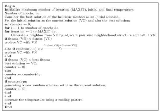
3.1. Variable neighborhood search algorithm The Variable Neighborhood Search (VNS) algorithm is one of the new meta-heuristic algorithms, which is based on systematic changes of the neighborhood structure. This algorithm searches for the optimum so-lution in combinatorial optimization problems. Unlike many other meta-heuristic algorithms, this algorithm is quite simple and requires fewer parameters to be tuned. Achieving high-quality solutions in a reasonable period of time and the simplicity of this method indicate the eciency of the algorithm. The VNS algorithm used in this study is derived from the basic case presented in [22] by Hansen and Mladenovic. The pseudo-code is shown in Figure 1.
The notion of VNS algorithm is based on the neighborhood structure changes, which prevents trap-ping into the localized optimization. As the problem and solution expand, the probability of trapping into a local minimum increases, hence the rst step in the VNS algorithm is dening a neighborhood structure that generates a neighborhood solution. Furthermore, since VNS was designed for approximating solutions of discrete and continuous optimization problems, it can be used for solving linear program problems, integer program problems, mixed integer program problems, nonlinear program problems, etc.
3.2. Simulated Annealing algorithm
Simulated Annealing (SA) algorithm is a local search algorithm which is not trapped into the local optimum.
Figure 2. SA pseudo-code.
Its easy usage, convergence, and special movement to avoid being trapped into the local optimum are some of the advantages of this algorithm [23]. The pseudo-code is shown in Figure 2. The basic idea behind SA is from cooling process of metals, which was rst suggested by Metropolis et al. [24] and optimized by Kirkpatricket et al. [25]. Despite generating a near-optimal solution, its outcome does not depend on the initial solution. Furthermore, even though it is an iterative algorithm, it does not have the common disadvantages of iterative methods as its upper limit execution time can also be specied. The basic idea originates in decreasing temperature of metals from an initial value of T0 to
a desired nal value of Tf in N required iterations,
which is called Epoch. The cooling pattern used here is given in Eq. (11), where Epoch is current number of iterations and r is a constant number between 0 and 1.
T1= T0 Epoch r: (11)
SA has attracted signicant attention as a suitable technique for optimization problems of large scale. The method has also been used successfully for designing complex integrated circuits and combinatorial mini-mization. Simulated annealing methods are also used for spaces with continuous control parameters. The SA algorithm presented in this paper includes some distinct features. First of all, it produces a random solution when the pre-determined number (pn) does not yield the best outcome. Secondly, several neighbor-hood structures are generated and selected randomly by the algorithm in each iteration. The main advantage of the SA algorithm, compared to VNS, is its speedy response. In general, the VNS algorithm provides an optimal solution when its number of iterations leans
towards innity. In the SA algorithm, however, an optimal result is generated during a xed number of iterations.
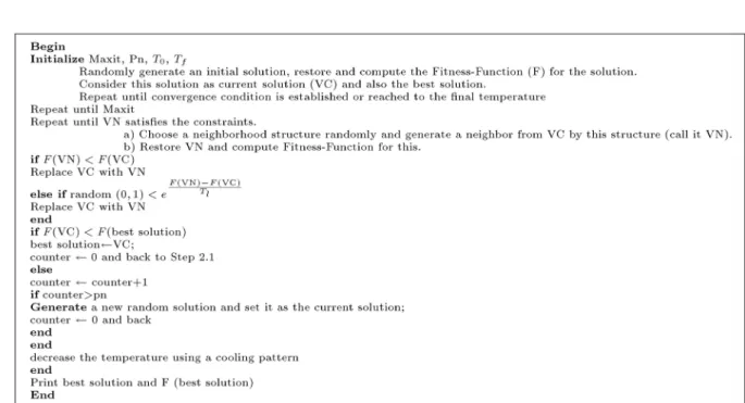
3.3. Hybrid SA algorithm
In the proposed SA algorithm, the positive attributes of both SA and VNS algorithms are used simultaneously. Unlike the VNS algorithm, which uses several neighbor-hood structures, the SA algorithm considers only one neighborhood structure. In the proposed algorithm, one of the neighborhood structures is selected randomly and a neighbor is generated from the current solution. This procedure not only reduces the chances of obtain-ing repetitive answers, but also reduces the probability of trapping into the local optimum. Furthermore, in addition to dening the stop criteria for the algorithm, the convergence condition is also dened. Under this condition, a big number is assumed for the outer loop (i.e., Epoch) and if the problem does not improve after a certain number of iterations, it is assumed converged and the improvement process ends [26]. The general outline of the given meta-heuristic is shown in Figure 3.
The objective function: The objective functions can be easily coded without requiring guide or competitive functions. However, the model is a multi-objective model and its objective functions are completely incompatible. When dealing with multi-objective modeling, one of the main challenges is to obtain a solution that optimizes all of its objective functions. Oftentimes, obtaining such an optimal solution becomes impossible because of the existence of conicts of interest among the objective functions. This study uses the Lp-metric method (with p =
Figure 3. Hybrid SA pseudo-code.
deviations of the existing objective functions from their optimal values as indicated in Eq. (12). In other words, when p is innity, to minimize LP
we need to minimize Z and the nal mathematical model can be denoted by Eqs. (12) and (13) subject to the initial constraints of the original model as indicated earlier in Constraints (6)-(10).
min Z = max
1
Z1 Z1
Z 1
; 2
Z2 Z2
Z 2
; 3
Z3 Z3
Z 3
= : (12)
S:T:
j Zj Z j
Z j
!
8j; (13)
assuming that:
1+ 2+ 3= 1: (14)
Solution representation: As iterative meta-heuristic algorithms require a structure for solution representation, this study purposes binary encoding, wherein each solution is represented by a string of 0 s and 1 s. This is rather a common approach and the following matrices are an example of a numerical solution for a scenario, in which there are three customers, three facilities, and up to 3 servers for each facility:
Xij=
2
41 0 01 0 0 0 0 1 3
5 ; Yju=
2
41 1 00 0 0 1 0 0 3 5 :
0 s and 1 s in matrix Xij indicate how to allocate
customers to facilities (Customer 1 and Customer 2 are assigned to the facility at potential Location 1 and Customer 3 to the facility at potential Location 3). Numbers in matrix Yju show how to allocate
servers to facilities (i.e., two servers are assigned to the rst facility and one server to the third one). In this solution, since the second facility has not yet been established, no server (i.e., the second row of the matrix Yju) and customer (i.e., the second
column of the matrix Xij) are assigned to it.
Constraints: The proposed model contains certain constraints that need to be dened so as to code its associated meta-heuristic algorithm. The model includes linear, nonlinear, equality, and inequality constraints. The strategy employed in this study is a \reject strategy", which has a simple approach of considering feasible solutions and declining infeasi-ble ones. This strategy has been used in dealing with Constraint (9). The model also includes other constraints (i.e., Constraints (6), (7), (8), and (10)), which can be included in the solution structure. Hence, we can generate feasible solutions for the problem utilizing the mentioned strategies.
4. Numerical examples
In order to clearly demonstrate convergence of the model and its eectiveness, and to objectively compare results of the two algorithms, several examples are designed and solved using the proposed hybrid SA and VNS algorithms. The solution algorithms are written in Matlab software 7.8.0 and tested on an Intel
Core i5 Computer having a CPU of 2.4 GHz and a RAM of 4 GB. For eective presentation purposes, after showing comprehensive solution for one sample example, the method is generalized and applied to other examples (1-6).
The following are considered for the sample ex-ample:
Set of customers including 30 points;
Set of potential locations for deployment of facilities including 10 points;
Transportation cost per distance unit per demand unit is assumed to be 1;
Maximum distance for a demand point to be covered by a facility is set to 5;
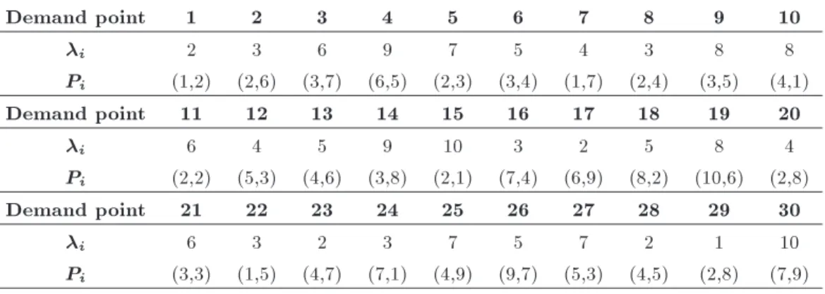
Maximum number of people in queue on the arrival of each customer, with probability of 0.9, is 5. Tables 1 and 2 indicate a comprehensive list of the relevant data. In designing the examples, we have considered existence of feasible area for each scenario.
Parameters of the algorithms have to be tuned prior to being applied to the examples. This means choosing the best possible values for parameters for the purpose of achieving optimal performance (the best possible performance of algorithm). These parameters may have great impact on the eciency and eective-ness of the algorithm. In general, providing optimum values for the parameters of a meta-heuristic algorithm is not possible and should be examined separately for each numerical example. There are various strategies
to tune the parameters and this research uses sequential strategy.
In the sequential strategy approach, each param-eter is investigated individually and their optimum val-ues are determined experimentally. As no interactive eects of parameters on each other can be determined in this approach, Design Of Experiments (DOE) is used to address this issue. In this way, the optimality of the parameters can be determined by considering the interaction between them.
The hybrid SA parameters, including MAXIT, T0,
and pn, need to be tuned. In the VNS algorithm, because there is just one parameter, the trial and error method can be adopted and it is used to compute op-timal value of the parameter. Table 3 shows the tuned values of these parameters for the sample example. Subsequently, the problem is solved with the Lp-metric method that requires the optimal value of each function separately. The optimal value and solution time of each function are shown in Table 4.
In this example, the convergence condition for the LP is considered passing 30 successive iterations without any change in the best objective function value. Table 5 shows the achieved outcomes from solving
Table 3. Optimal values of the hybrid SA algorithm parameters for the sample example.
Parameter Upper-lower Optimum value
Maxit 100-500 300
T0 1000-4000 2000
pn 10-20 10
Table 1. Relevant data of the potential locations for the sample example.
Potential location 1 2 3 4 5 6 7 8 9 10
qj 2 4 1 3 5 3 2 5 4 3
Fj 1000 1200 1300 1400 1500 1600 1700 1800 1900 1800
Cj 5 4 3 2 8 2 3 4 5 7
j 4 6 5 10 3 9 6 5 4 3
Hj (4,6) (3,2) (1.5,4) (6,6) (5,1) (9,2) (6,3) (3,6) (1,8) (5,2) Table 2. Relevant data of demand points for the sample example.
Demand point 1 2 3 4 5 6 7 8 9 10
i 2 3 6 9 7 5 4 3 8 8
Pi (1,2) (2,6) (3,7) (6,5) (2,3) (3,4) (1,7) (2,4) (3,5) (4,1)
Demand point 11 12 13 14 15 16 17 18 19 20
i 6 4 5 9 10 3 2 5 8 4
Pi (2,2) (5,3) (4,6) (3,8) (2,1) (7,4) (6,9) (8,2) (10,6) (2,8)
Demand point 21 22 23 24 25 26 27 28 29 30
i 6 3 2 3 7 5 7 2 1 10
Table 4. Optimum value and solution time of each function for the sample example. Hybrid SA algorithm VNS algorithm Optimum
value
Solution time (s)
Optimum value
Solution time (s)
First function (servers) 18 2.50 11 18.77
Second function (cost) 15311 2.46 15310 19.20
Third function (quality) 97 2.48 97 19.50
Table 5. Achieved outcomes from solving the LP with dierent combinations of the weights for the sample example. j
Hybrid SA algorithm VNS algorithm Branch and bound
Optimum value
Solution time
(s)
Z1 Z2 Z3 Optimum value
Solution time
(s)
Z1 Z2 Z3 Optimum value
Solution time
(s)
Z1 Z2 Z3 0.6-0.1-0.3 0.0096 4.03 22 15500 51 8.567e-4 3.71 18 15441 34 1,002e-5 8 18 15440 51 0.1-0.3-0.6 0.0286 5.41 23 15451 55 1.6e-3 4.86 19 15392 42 3,001e-5 11 19 15392 55 0.3-0.6-0.1 0.0572 4.76 20 15604 51 7.594e-4 4.72 19 15329 34 3,023e-5 9 19 15317 51
Figure 4. Improvement process for the proposed hybrid SA algorithm regarding the sample example with equal to (a) 0.3, 0.1, and 0.6, (b) 0.6, 0.3, and 0.1, and (c) 0.1, 0.6, and 0.3.
Figure 5. Improvement process for the VNS algorithm regarding the sample example with equal to (a) 0.3, 0.1, and 0.6, (b) 0.6, 0.3, and 0.1, and (c) 0.1, 0.6, and 0.3.
the LP with dierent combinations of the weights for the sample example. Also, in this table, the achieved outcomes from solving the LP with branch and bound method are shown to compare the proposed method with an exact method. It can be seen that outcomes of these two methods are very close to those of the optimal solutions. Figures 4 and 5 show the improvement process of these six cases wherein the horizontal axis represents the number of iterations, in which the algorithm shows improvement and the vertical axis represents the best value of the objective
function. Now that convergence of the two algorithms is demonstrated, we need to calculate an index called RPI for the purpose of comparing the two algorithms. The next section discusses a general process of calcu-lating the index and shows the associated results for the above-mentioned examples.
5. RPI method for comparing the algorithms As mentioned earlier, the RPI is used to compare the eciency of algorithms in solving problems. The
general formula of the index is represented in Eq. (15): RPI =best objective valuebest worst : (15) The following steps are used to calculate the RPI for eciency comparison:
Each algorithm is run ve times for a numerical example of the problem;
The objective function values are acquired for each algorithm during each run;
The best and the worst objective function values are identied;
RPI is calculated for each objective function in each run;
The average value of RPI ( R ) is calculated for each algorithm.
As the process shows in Table 6, the index for the sample example is calculated. All the above steps are repeated for the given six numerical examples, the results of which are summarized in Table 7. The comparative statistical tests are used to compare R s. In this study, the 2-sample t-test with a condence level
Table 6. Results of R for the sample example.
j
SA VNS
LP objective
value
LP solution time (S)
LP objective
value
LP solution time (S)
0.6,0.1,0.3
0.0096 2.3 1.2e-4 4.6
0.0096 2.9 6.3e-4 3.5
0.0097 2.3 5.7e-4 2.7
0.0095 4.7 6.9e-4 2.8
0.0095 4.9 0.0e-0 7.0
R 0.4000 0.43 5.82e-1 0.32
0.1,0.3,0.6
0.0282 2.2 1.1e-4 5.4
0.0286 2.7 2.0e-3 2.8
0.0283 5.2 5.8e-4 4.7
0.0285 4.5 1.4e-3 4.1
0.0285 8.1 1.7e-3 4.4
R 0.5500 0.40 5.54e-1 0.57
0.3,0.6,0.1
0.0571 2.2 0.0e-0 4.8
0.0575 3.5 3.2e-3 7.3
0.0574 4.0 1.0e-3 6.8
0.0574 3.2 4.9e-3 6.9
0.0573 2.6 1.2e-3 3.5
R 0.6000 0.50 4.2e-3 0.62
of 0.95 is used and the following assumptions are also tested. The rst investigated hypothesis is to identify any dierences between the qualities of the obtained solution and the two algorithms.
Thus, H0and H1are as follows:
H0: SA VNS; H1: SA< VNS:
Hypothesis 1 (H1) means that SA algorithm has better
performance than VNS. This is because the mean objective function value (as the solution quality) of SA was assumed to be less than or equal to that of VNS. The P -Value turns out to be equal to 0.308, which implies that with a 95% condence, H1 cannot
be accepted.
Aside from the quality of the solutions obtained from an algorithm, time to achieve the optimal solution is also an important factor in selecting an algorithm. Therefore, the second hypothesis is dened by:
H0: tSA tVNS; H1: tSA< tVNS:
Hypothesis 1 (H1) means that SA algorithm reaches
the corresponding solution faster than VNS. This is again because the mean time for SA was assumed to be less than or equal to that for VNS. As P -Value turns out to be equal to 0.026, it indicates that by 95% condence, H1 can be accepted.
6. Conclusion
In this paper, several potential locations were consid-ered and we aimed at locating a number of facilities at those locations, each equipped with some servers. The total number of servers was considered unknown, but the maximum number of servers that could be allocated to each facility was specied and when deploying a location, at least one server was allocated to it. We proposed a model based on the customers' perspective and optimized its three objective functions of:
1. Minimizing the total number of assigned servers;
2. Minimizing the total transportation and the facility deployment costs;
3. Maximizing the quality of service from the cus-tomers' point of view, in order to attain our objectives.
It was shown that the hybrid SA algorithm attains near-optimal solutions more eciently and sequential strategy was used for tuning of its parameters. Some numerical examples, which were designed to evalu-ate the algorithm's performance, were demonstrevalu-ated. Finally, the two algorithms of SA and VNS were compared by the RPI method in order to identify the best performing algorithm. The results indicated that there was no signicant dierence between the qualities
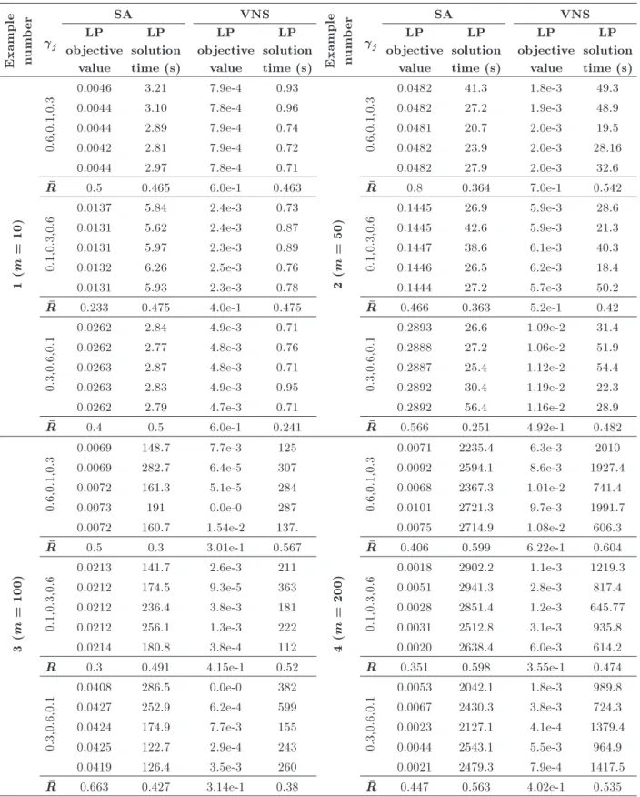
Table 7. Results of R for examples 1-6.
Example num
b
er
j
SA VNS
Example num
b
er
j
SA VNS
LP objective
value
LP solution time (s)
LP objective
value
LP solution time (s)
LP objective
value
LP solution time (s)
LP objective
value
LP solution time (s)
1
(m
=
10)
0.6,0.1,0.3
0.0046 3.21 7.9e-4 0.93
2
(m
=
50)
0.6,0.1,0.3
0.0482 41.3 1.8e-3 49.3
0.0044 3.10 7.8e-4 0.96 0.0482 27.2 1.9e-3 48.9
0.0044 2.89 7.9e-4 0.74 0.0481 20.7 2.0e-3 19.5
0.0042 2.81 7.9e-4 0.72 0.0482 23.9 2.0e-3 28.16
0.0044 2.97 7.8e-4 0.71 0.0482 27.9 2.0e-3 32.6
R 0.5 0.465 6.0e-1 0.463 R 0.8 0.364 7.0e-1 0.542
0.1,0.3,0.6
0.0137 5.84 2.4e-3 0.73
0.1,0.3,0.6
0.1445 26.9 5.9e-3 28.6
0.0131 5.62 2.4e-3 0.87 0.1445 42.6 5.9e-3 21.3
0.0131 5.97 2.3e-3 0.89 0.1447 38.6 6.1e-3 40.3
0.0132 6.26 2.5e-3 0.76 0.1446 26.5 6.2e-3 18.4
0.0131 5.93 2.3e-3 0.78 0.1444 27.2 5.7e-3 50.2
R 0.233 0.475 4.0e-1 0.475 R 0.466 0.363 5.2e-1 0.42
0.3,0.6,0.1
0.0262 2.84 4.9e-3 0.71
0.3,0.6,0.1
0.2893 26.6 1.09e-2 31.4
0.0262 2.77 4.8e-3 0.76 0.2888 27.2 1.06e-2 51.9
0.0263 2.87 4.8e-3 0.71 0.2887 25.4 1.12e-2 54.4
0.0263 2.83 4.9e-3 0.95 0.2892 30.4 1.19e-2 22.3
0.0262 2.79 4.7e-3 0.71 0.2892 56.4 1.16e-2 28.9
R 0.4 0.5 6.0e-1 0.241 R 0.566 0.251 4.92e-1 0.482
3
(m
=
100)
0.6,0.1,0.3
0.0069 148.7 7.7e-3 125
4
(m
=
200)
0.6,0.1,0.3
0.0071 2235.4 6.3e-3 2010
0.0069 282.7 6.4e-5 307 0.0092 2594.1 8.6e-3 1927.4
0.0072 161.3 5.1e-5 284 0.0068 2367.3 1.01e-2 741.4
0.0073 191 0.0e-0 287 0.0101 2721.3 9.7e-3 1991.7
0.0072 160.7 1.54e-2 137. 0.0075 2714.9 1.08e-2 606.3
R 0.5 0.3 3.01e-1 0.567 R 0.406 0.599 6.22e-1 0.604
0.1,0.3,0.6
0.0213 141.7 2.6e-3 211
0.1,0.3,0.6
0.0018 2902.2 1.1e-3 1219.3
0.0212 174.5 9.3e-5 363 0.0051 2941.3 2.8e-3 817.4
0.0212 236.4 3.8e-3 181 0.0028 2851.4 1.2e-3 645.77
0.0212 256.1 1.3e-3 222 0.0031 2512.8 3.1e-3 935.8
0.0214 180.8 3.8e-4 112 0.0020 2638.4 6.0e-3 614.2
R 0.3 0.491 4.15e-1 0.52 R 0.351 0.598 3.55e-1 0.474
0.3,0.6,0.1
0.0408 286.5 0.0e-0 382
0.3,0.6,0.1
0.0053 2042.1 1.8e-3 989.8
0.0427 252.9 6.2e-4 599 0.0067 2430.3 3.8e-3 724.3
0.0424 174.9 7.7e-3 155 0.0023 2127.1 4.1e-4 1379.4
0.0425 122.7 2.9e-4 243 0.0044 2543.1 5.5e-3 964.9
0.0419 126.4 3.5e-3 260 0.0021 2479.3 7.9e-4 1417.5
R 0.663 0.427 3.14e-1 0.38 R 0.447 0.563 4.02e-1 0.535
of the solutions obtained from the two algorithms; but as far as convergence and solution time were concerned, Simulated Annealing (SA) algorithm had higher performance than the Variable Neighborhood Search (VNS) algorithm. Future research on this topic
may focus on customer service and arrival using other queuing models. Additionally, hierarchical models can be deployed to prioritize the requests and apply more restrictions on economic, competitive, or geographical conditions.
Table 7. Results of R for examples 1-6 (continued).
Example num
b
er
j
SA VNS
Example num
b
er
j
SA VNS
LP objective
value
LP solution time (s)
LP objective
value
LP solution time (s)
LP objective
value
LP solution time (s)
LP objective
value
LP solution time (s)
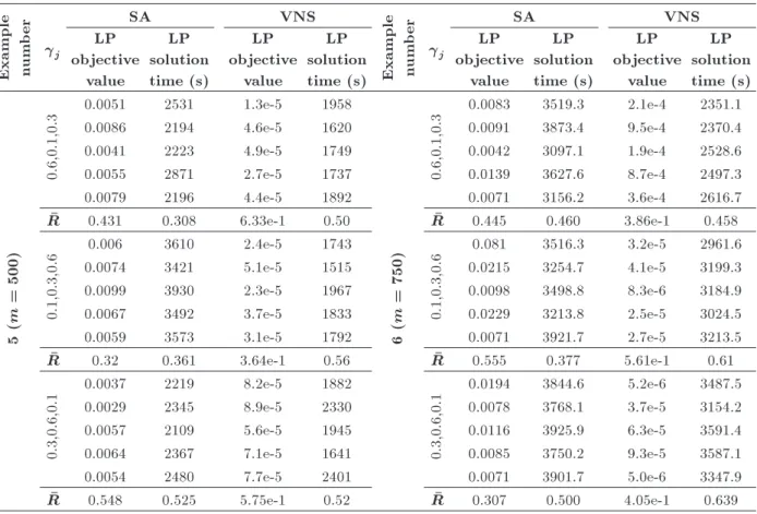
5
(m
=
500)
0.6,0.1,0.3
0.0051 2531 1.3e-5 1958
6
(m
=
750)
0.6,0.1,0.3
0.0083 3519.3 2.1e-4 2351.1
0.0086 2194 4.6e-5 1620 0.0091 3873.4 9.5e-4 2370.4
0.0041 2223 4.9e-5 1749 0.0042 3097.1 1.9e-4 2528.6
0.0055 2871 2.7e-5 1737 0.0139 3627.6 8.7e-4 2497.3
0.0079 2196 4.4e-5 1892 0.0071 3156.2 3.6e-4 2616.7
R 0.431 0.308 6.33e-1 0.50 R 0.445 0.460 3.86e-1 0.458
0.1,0.3,0.6
0.006 3610 2.4e-5 1743
0.1,0.3,0.6
0.081 3516.3 3.2e-5 2961.6
0.0074 3421 5.1e-5 1515 0.0215 3254.7 4.1e-5 3199.3
0.0099 3930 2.3e-5 1967 0.0098 3498.8 8.3e-6 3184.9
0.0067 3492 3.7e-5 1833 0.0229 3213.8 2.5e-5 3024.5
0.0059 3573 3.1e-5 1792 0.0071 3921.7 2.7e-5 3213.5
R 0.32 0.361 3.64e-1 0.56 R 0.555 0.377 5.61e-1 0.61
0.3,0.6,0.1
0.0037 2219 8.2e-5 1882
0.3,0.6,0.1
0.0194 3844.6 5.2e-6 3487.5
0.0029 2345 8.9e-5 2330 0.0078 3768.1 3.7e-5 3154.2
0.0057 2109 5.6e-5 1945 0.0116 3925.9 6.3e-5 3591.4
0.0064 2367 7.1e-5 1641 0.0085 3750.2 9.3e-5 3587.1
0.0054 2480 7.7e-5 2401 0.0071 3901.7 5.0e-6 3347.9
R 0.548 0.525 5.75e-1 0.52 R 0.307 0.500 4.05e-1 0.639
References
1. Toregas, C., Swain, R., ReVelle, C. and Bergman, L.
\The location of emergency service facilities", Opera-tions Research, 19, pp. 1363-1373 (1971).
2. Shanthikumar, J.G. and Yao, D.D. \Optimal server
allocation in a system of multi-server stations", Man-agement Science, 33, pp. 1173-1191 (1978).
3. Hakimi, S.L. \On locating new facilities in a
compet-itive environment", European Journal of Operational Research, 12, pp. 29-35 (1983).
4. ReVelle, C. and Hogan, K. \A reliability-constrained
sitting model with local estimates of busy fractions", Environment and Planning B: Planning and Design, 15, pp. 143-152 (1988).
5. Marianov, V. and ReVelle, C. \The queuing
probabilis-tic location set covering problem and some extensions", Socio-Economic Planning Sciences, 28, pp. 167-178 (1994).
6. Marianov, V., Serra, D. and Revelle, C. \Location of
hubs in a competitive environment", European Journal of Operational Research, 114, pp. 363-371 (1999).
7. Marianov, V. and Serra, D. \Hierarchical
location-allocation models for congested systems", European Journal of Operational Research, 135, pp. 195-208 (2000).
8. Marianov, V. and Serra, D. \Location-allocation of
multiple-server service center with constrained queues
or waiting time", Annals of Operations Research, 111, pp. 35-50 (2002).
9. Shavandi, H. and Mahlooji, H. \A fuzzy queuing
loca-tion model with a genetic algorithm for congested sys-tems", Applied Mathematics and Computation, 181, pp. 440-456 (2006).
10. Rajagopalan, H.K. and Saydam, C. \A minimum
expected response model: Formulation, heuristic so-lution, and application", Socio-Economic Planning Sciences, 43, pp. 253-262 (2009).
11. Restrepo, M., Henderson, S.G. and Topaloglu, H.
\Erlang loss models for the static deployment of ambulances", Health Care Management Science, 12, pp. 67-79 (2009).
12. Liu, Q. and Xu, J. \A study on facility
location-allocation problem in mixed environment of random-ness and fuzzirandom-ness", Journal of Intelligent Manufactur-ing, 3, pp. 389-398 (2011).
13. Chanta, S., Mayorga, M.E. and Mclay, L.A.
\Improv-ing emergency service in rural areas: a bi-objective covering location model for EMS systems", Annals of Operation Research, pp. 1027-1054 (2011).
14. Arnaout, J.P. \Ant colony optimization algorithm
for the Euclidean location-allocation problem with unknown number of facilities", Journal of Intelligent Manufacturing, 24, pp. 45-54 (2011).
server location problem", Computers and Operations Research, 38, pp. 694-701 (2011).
16. Li, X., Zhao, Z., Zhu, X. and Wyatt, T. \Covering
models and optimization techniques for emergency response facility location and planning: a review", Mathematic Meta Operations Research, 74, pp. 2811-310 (2011).
17. Benneyan, J.C., Musdal, H., Ceyhan, M.E., Shiner,
B. and Watts, B.V. \Specialty care single and multi-period location allocation models within the veterans health administration", Socio-Economic Planning Sci-ences, 46, pp. 136-148 (2012).
18. Rahmati, S.H.A., Hajipour, V. and Akhavanniaki,
S.T. \A soft computing pareto based meta heuristic algorithm for a multi objective multi server facility location problem", Applied Soft Computing, 13, pp. 1728-1740 (2013).
19. Mousavi, S.M. and Akhavan Niaki S.T. \Capacitated
location allocation problem with stochastic location and fuzzy demand: A hybrid algorithm", Applied Mathematical Modeling, 37, pp. 5109-5119 (2013).
20. Adler, N., Hakkert, A.S., Kornbluth, J., Raviv, T. and Sher, M. \Location-allocation models for trac police patrol vehicles on an interurban network", Ann. Oper. Res. (2013).
21. Goswami, V. \Analysis of discrete-time multi-server
queue with balking", International Journal of Man-agement Science and Engineering ManMan-agement, 9(1), pp. 21-31 (2014).
22. Hansen, P. and Mladenovic, N. \Variable
neighbor-hood search for the p-median", Location Science, 5, pp. 207-226 (1997).
23. Hajakbari, A. \Simulated annealing approach for
solv-ing stock cuttsolv-ing problem", IEEE International Con-ference on Systems Man and Cybernetics ConCon-ference Proceedings (1990).
24. Metropolis, N., Rosenbluth, A.W., Rosenbluth, M.N.,
Teller, A.H. and Teller, E. \Equation of state calcula-tion by fast computing machines", Journal of Chem. Phys., 21, pp. 1087-1091 (1953).
25. Kirkpatrick, S., Gellat, C.D. and Vecchi, M.P.
\Opti-mization by simulated annealing", Science, 220, pp. 671-680 (1983).
26. Deb, S.K. \Solution of facility layout problems with
pickup/drop-o locations using random search tech-niques", International Journal of Production Research (2005).
Biographies
Maryam Ghobadi is a PhD student in the Depart-ment of Industrial Engineering at Kordestan University of Iran. She received her MSc degree in Industrial Engineering from Alzahra University in 2013. Her current research interests include location and supply chain management.
Mehdi Seifbarghy is Professor in the Department of Industrial Engineering at Alzahra University of Iran and presently serves as the Vice President of Academic Aairs. In teaching, he has been focusing on location and facility layout problems and supply chain management. In research, his current interests include location and supply chain management. Dr. Seifbarghy received his PhD degree in Industrial Engineering from Sharif University of Technology, Tehran, Iran.
Reza Tavakkoli-Moghaddam is Professor of In-dustrial Engineering at University of Tehran, Iran. He obtained his PhD in Industrial Engineering from the Swinburne University of Technology in Melbourne (1998). He is an Associate Member at Academy of Sciences in Iran and serves as Editorial Board Member of the International Journal of Engineering and Iranian Journal of Operations Research. He was the recipient of the 2009 and 2011 Distinguished Researcher Awards and the 2010 Distinguished Applied Research Award at University of Tehran, Iran. He was selected as National Iranian Distinguished Researcher in 2008 and 2010 in Iran. Professor Tavakkoli-Moghaddam has published 4 books, 15 book chapters, and more than 500 papers in reputable academic journals and conferences.
Davar Pishva is a Professor in ICT at the College of Asia Pacic Studies, Ritsumeikan Asia Pacic Univer-sity (APU) Japan. In teaching, he has been focusing on information security, technology management, VBA for modelers, structured decision making and carries out his lectures in an applied manner. In research, his current interests include biometrics; e-learning, environmentally sound and ICT enhanced technologies. Dr. Pishva received his PhD degree in System Engi-neering from Mie University, Japan. He is a Senior Member of IEEE, a member of IEICE (Institute of Electronics Information & Communication Engineers), and University & College Management Association.