Sorg_unc_0153M_16974.pdf

IDENTIFYING SUSTAINABLE SUBSTRATES FOR SUBTIDAL OYSTER REEF CONSTRUCTION

Gregory Dennis Sorg

A thesis submitted to the faculty at the University of North Carolina at Chapel Hill in partial fulfillment of the requirements for the degree of Master of Science in the Department of Marine

Sciences.

Chapel Hill 2017

Approved by:

ii ©2017

iii

ABSTRACT

Gregory Dennis Sorg: Identifying Sustainable Substrates for Subtidal Oyster Reef Construction (Under the direction of Niels Lindquist)

Historically, oyster shell has been the preferred substrate for reef foundations in

restoration efforts targeting the eastern oyster Crassostrea virginica. Alternative reef foundation substrates are desirable due to increasing costs of oyster shell. Further, carbonate (CaCO3) based

substrates are susceptible to degradation by bioeroders (e.g. Clionid sponges). Oyster

demographics, Clionid infestation of oysters and substrates, and characterization of predation sources on juvenile oysters were tracked in a long-term study (54 months) of 80 subtidal oyster reefs constructed in 2012 across salinity gradients in two North Carolina estuaries. Reefs had foundations of either CaCO3-based (oyster shell or marl pebble) or nonCaCO3-based (concrete

cobble or granite pebble) substrates. Results indicated estuarine location and reef foundation composition interacted to determine the fate of oyster communities. Continued use of CaCO3

iv

v

ACKNOWLEDGEMENTS

First, I thank my advisor, Dr. Niels Lindquist who has provided countless hours of guidance in the field as well as in the writing process. I also thank my committee members, Drs. Steve Fegley and Joel Fodrie for their thoughtful insights throughout this project. Dr. Fegley has provided exceptionally valuable advice on statistical analyses.

I will be eternally grateful for the assistance, companionship, and insights of two Carteret County commercial shellfishers, Adam Tyler and David “Clammerhead” Cessna. These

individuals have volunteered their expertise beyond paid time. Their love for their estuarine waters is infectious and by working with them on this and other projects, I feel I have gained a unique perspective not often afforded to young scientists. Their hard work on building the reef foundations is will always be an understatement. Others who assisted with reef building effort include, but is not limited to, Eamon Kromka, Stacy Davis, Justin Ridge, Glenn Safrit, and Robert Dunn.

vi

TABLE OF CONTENTS

LIST OF TABLES………vii

LIST OF FIGURES………..viii

INTRODUCTION…….………..1

MATERIALS AND METHODS………...6

Reef Construction………6

Sample Collection………8

Length Frequency Distributions………10

Regression Tree Analysis………..11

Cause of Death………...13

RESULTS…………..………15

Length Frequency Distributions………15

Regression Tree Analysis………..18

Cause of Death………...28

DISCUSSION….…….………..30

APPENDIX 1: LENGTH FREQUENCY DISTRIBUTIONS………..42

APPENDIX 2: REGRESSION TREE ANALYSES ………...82

APPENDIX 3: CAUSE OF DEATH OF BOXES (JUNE 2015 & DECEMBER 2016)………..84

vii

LIST OF TABLES

viii

LIST OF FIGURES

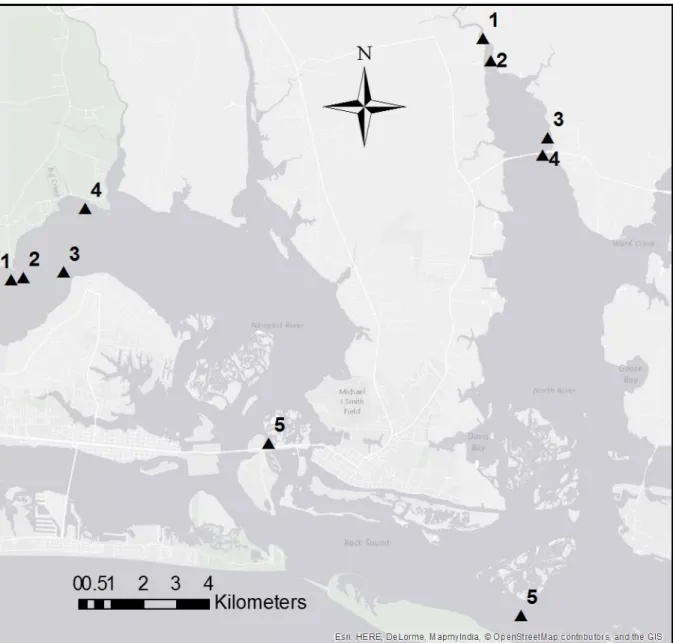
Figure 1. Study Site Locations in Newport and North River Estuaries……….7

Figure 2. Regression Tree of Live Oyster Density………...19

Figure 3. Regression Tree of Small Live Oyster Density……….20

Figure 4. Regression Tree of Dead Oyster Density………..22

Figure 5. Regression Tree of Small Dead Oyster Density………23

Figure 6. Regression Tree of Live Boring Sponge in Reef Substrate………...24

Figure 7. Regression Tree of Live Boring Sponge in Live Oysters………..25

Figure 8. Regression Tree of Dead Boring Sponge in Live Oysters………26

Figure 9. Regression Tree of Dead Cliona spp. (non-Cliona celata) in Live Oysters………….27

1

INTRODUCTION

Salinity tolerance is a basic driver of species distributions in estuarine systems (Wells 1961, Crain et al. 2004, Galván et al. 2016 and references therein). The eastern oyster

Crassostrea virginica, hereafter oyster, is a euryhaline estuarine species with salinity tolerances from 5-40 (Galstoff 1964). However, the realized distribution of subtidal oyster reefs is typically limited to the polyhaline regions of the upper to mid-estuary as a result of marine adapted pests and predators exerting top-down controls on the oyster populations in high salinity waters (Grave 1904, Wells 1959, Walles 2016) and the increased physical stresses of a oligohaline environment (Galstoff 1964).

2

In North Carolina, the commercial harvest of wild oysters was valued at ~$4 million in 2015 (NCDMF). The number of bushels of oysters harvested commercially in NC was

approximately 119,000 in 2015, only a fraction of the historic peak of 806,561 bushels occurring in 1902 (NC DMF). By 1910, only ~262,000 bushels were harvested.

Planktonic oyster larvae require firm substrates onto which they for the duration of their life. The restoration of oysters involves placing firm substrates on the benthos of estuaries, ideally in locations suitable to the persistence of the population of restored oysters.

In response to the rapid, early 20th century decline in oyster harvest in NC, a state funded cultch-planting program began in 1915 (Marshall et al. 1999). The traditional methods of the cultch planting in NC involved the placement of loose oyster shells onto the benthos in regions requested by commercial shellfishers. By 1946, a NC law required that oyster shucking houses contribute at least 50% of their shell material to the state run Oyster Rehabilitation Program, diverting shell that would have likely gone into chicken feed and roads back into the estuaries (Marshall et al. 1999). However, the increasing price and decreased availability of loose oyster shell, especially during the second half of the 20th century, led to the exploration of alternative substrates for oyster reef construction in NC and other coastal states (Marshall et al. 1999, Luckenbach et al. 1999). Typically, other molluscan shells or other calcium carbonate-based materials (i.e. limestone, marl) were substituted for loose oyster shells in restoration practice (Marshall et al. 1999).

Soniat et al. (1991) suggested that alternative substrates for oyster restoration should be biologically acceptable for the recruitment of oysters and environmentally acceptable. Studies gauging the performance of alternative substrates to oyster shells examined a variety of

3

and marl (a carbonate rock), manufactured concrete structures, crushed concrete, and even shredded tire waste and derelict porcelain bathroom fixtures (Soniat et al. 1991, Soniat and Burton 2005, Brown et al. 2014, Theuerkauf et al. 2014, George et al. 2014). Overall, most studies found if differences in substrate preference were observed, oyster spat typically favored settlement onto carbonate-based substrate (Soniat and Burton 2005, George et al. 2014). This is not surprising given that oyster shells are primarily composed of carbonate. However,

Theuerkauf et al. (2014) found that Oyster Castle™ concrete structures recruited more oyster spat when compared with loose oyster shell. The majority of these studies limited the settlement period to less than 3 months and reported net settlement only, with no consideration of spat survival or long-term reef development.

As a means of evaluating the long-term efficacy of different substrate materials, a “snapshot” study by Brown and co-workers (2014) examined oyster populations on reefs of differing ages and deployed during different years/seasons. This study assumed younger reefs were representative of the older reefs at earlier time-steps. This critical assumption was likely not met due to complex physical-biological interactions that occur during reef development, including annual variability of environmental conditions, disease, and oyster spat sets (Grave 1904, Kimmel and Newell 2007). Additionally, comparisons of substrate performance generally focused on similar sites and rarely explore the influences of ecologically relevant environmental gradients, including salinity and/or aerial exposure times (Ridge et al. 2015, Walles et al. 2016.). For example, Fodrie et al. (2014) found that reefs with highest oyster larval settlement

4

In 2004, the continued low harvest of oysters prompted the NC Division of Marine Fisheries, NC DMF, to develop a series 1-5 hectare reserves as broodstock sanctuaries in Pamlico Sound. NC DMF and their restoration partners created reef foundations from large mounds of marl boulders within these reserves. Initial oyster population trajectories in these sanctuaries were promising with large numbers of oysters growing into breeding adult size classes (Puckett and Eggleston 2012). However, from 2007 - 2010, oyster populations in the two large eastern Pamlico Sound sanctuaries declined precipitously (NC DMF, unreported data; Dunn et al. 2014 and sources cited therein). After conducting an underwater survey of the sanctuary near Ocracoke with NC DMF staff and examining marl rock samples from these sanctuaries, Lindquist (UNC-IMS) hypothesized that the marl mounds had become heavily infested by oyster pests common in high salinity waters, including oyster drills and Clionid boring sponges (N. Lindquist, personal communication). Lindquist suspected that the porous limestone (based) boulders were particularly susceptible to infestation by carbonate-eroding organisms, most notably Clionid sponges, in higher salinity environments and Polydora spp. polychaetes in lower salinity waters.

For this study, we tested the performance of four substrates, two carbonate-based

materials: oyster shell and marl, both expected to be susceptible to carbonate bioeroders, and two non-carbonate based materials: crushed concrete and granite, predicted to be impervious to bioeroders. We tested the relative effectiveness of these reef foundation materials for promoting sustainable subtidal oyster populations across broad salinity gradients in two neighboring

5

Initial project findings, reported by Dunn et al. (2014), focused on substrate performance (i.e. live oyster numbers and sizes and boring sponge infestation of substrates) on constructed reef 3-12 months post-construction. Dunn and coworkers’ (2014) early-stage surveys found minimal boring sponge occurrences on the constructed reefs. At 3 months post construction, the largest juvenile oysters were observed at the highest salinity sites in both estuaries. Further, at this time step, the greatest oyster densities were found on the high salinity reefs. However, by 12 months post-construction, no significant differences in live oyster sizes or live oyster densities were found among the different reef foundation materials at all sites. Here, I report results obtained from my surveys of these reefs 24 to 54 months post-construction using more extensive survey methodologies compared to those of Dunn et al. (2014). My updated methodology

included metrics for both live and dead oysters and boring sponge infestation levels in the substrate, live oysters, and probable sources of mortality for recently dead oysters.

6

MATERIALS AND METHODS

Reef Construction

In May 2012, Lindquist, UNC-IMS students and technicians, and two Carteret County commercial fishermen – Adam Tyler and David “Clammerhead” Cessna - constructed 80 subtidal oyster reef foundations were at five sites each in both the North River and Newport River estuaries in Carteret County, North Carolina (Figure 1). At each site, eight reefs were created with two reefs of each of the four substrate types with their depth at MLLW ranging from 0.5 to 1.0 m. Each reef foundation had a footprint of 2 m x 2 m and 0.25 m relief. Reefs were placed in the linear order of granite-marl-shell-concrete-granite-marl-shell-concrete with 2-m spacing between the reefs. Best efforts were made to place reefs on firm benthic substrate, for example sand or firm mud to limit sinking and burial of reef material and not over existing hard substrates, such as oyster shell reefs. However, Newport River Site 3 and North River Site 5 experienced partial periodic burial by flocculant mud and sand, respectively.

The five sites in each estuary were selected to span a wide range of salinity

7

of characterizing the salinity regimes among out test sites, we turned to Fodrie and colleagues (UNC-IMS) who were maintaining conductivity/temperature sensors in the North and Newport River estuaries from 2013 until 2015. At time of publishing, these data were not vetted for analysis.

8

Sample Collection

Long-term oyster development and potential interactions between substrate types and biological responses was determined by removing substrate material from the reef foundations 24 months (May 2014), 28 months (September 2014), 36 months (June 2015), and 54 months (December 2016) post-reef construction. On each sampling compaign, substrates and attached oysters were removed from the reefs in a single day for each estuary, and the estuaries were generally sampled over a consecutive 2-day period. The abbreviation of NoR and NpR will be used to refer to the North River estuary and Newport River estuary, respectively. Site numbers are included in the abbreviation. During the December 2016 sampling event, NpR5 was not accessible on the same day as the other Newport River samples due to an extreme low tide. This site was sampled using a kayak three days after the other collections from the Newport River. No samples were collected at NoR1 in May 2014 due to an oversight error.

The September 2014 sampling occurred after an extensive and extended freshet occurred in the Newport River estuary, and to a lesser extent in the North River. This sampling allowed exploration of the effects of a large, extended freshwater pulse on oyster and sponge

demographics. A similar freshet event occurred during the summer of 2015. Continuous salinity records indicate the 2015 event was not as severe as the 2014 event (Tice-Lewis, Greg Sorg, unpubl. data).

9

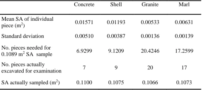
depth, which limited the potential for visual biases. The number of pieces of each substrate type collected was predetermined (20 Granite, 17 Marl, 9 Shell, 7 Concrete) in accordance with Dunn and co-workers (2014). These numbers of substrate pieces were determined to have ~ 0.10 m2 of substrate surface area for each material type (Dunn et al. 2014) (Table 1).

When removed from the reef complex, individual pieces were placed into a weighted bushel-size fish basket or directly onto the research vessel. Samples were then placed into a labeled plastic bag, sealed, and brought to UNC Institute of Marine Science for scoring. Samples were stored in a -5°C freezer until processed.

Table 1. Experimental oyster reef sampling protocol based on surface area (SA) of individual reef substrate pieces, standardized to a common sample size via weight:area conversion using aluminum foil. (From Dunn et al. 2014)

Concrete Shell Granite Marl

Mean SA of individual

piece (m2₎ 0.01571 0.01193 0.00533 0.00631

Standard deviation 0.00510 0.00387 0.00136 0.00139

No. pieces needed for

0.1089 m2 SA sample 6.9299 9.1209 20.4246 17.2599

No. pieces actually

excavated for examination 7 9 20 17

SA actually sampled (m2_{) 0.1100 0.1075 0.1066 0.1073}

10

valve lengths measured (umbo to distal shell end). Oysters with articulated valves but no oyster tissue present (‘boxes’) were included in the dead oyster category. Only dead oysters, boxes or left attached valves, were scored if no heavy fouling was observed on the individual, suggesting its death occurred relatively close to the sampling date. The length of boring sponge infestation was measured along the shell height of each oyster and was categorized as live or dead. Live sponge was detected by observing sponge tissue within the galleries typical of Clionid sponge infestation of carbonate-based materials. Dead sponge was assumed if no sponge tissue occupied the galleries. Further, I characterized the type of sponge infestation as either “large hole” or “small hole” describing the relative diameter of the shell surface perforation made by different Clionid sponge species. Large diameter shell perforations (~2 mm) are created by the high-salinity adapted Clionid sponge, Cliona celata. Small diameter shell perforations (~ 0.5mm) are created by multiple, lower salinity adapted Cliona spp. Thus, the boring sponge species found at a site is indicative of the general salinity regime (Hopkins 1956, Wells 1959).

Length Frequency Distributions

11

shell were categorized as containing live sponge in the LFD plots generation. The ratio of the number of live oysters to the number of dead oysters to numbers for each substrate type included on the LFDs for each site.

The percent cover of live sponge on the substrate was estimated and included on each LFD plot. Among the non-carbonate substrates, boring sponge did not penetrate into the granite, and only into calcium carbonate aggregate in the concrete, which were rarely observed. Thus, boring sponge penetration and occupation of crushed concrete was essentially zero. For oyster shell, the mean percent area of each shell showing surface perforations caused by boring sponges was calculated as the L x W of the shell with boring sponge perforations divided by the oyster shell length and width at the mid-shell point. For marl, percent cover of boring sponge, both live and dead, on individual pieces of marl was estimated visually and confirmed by a second individual. This dual independent scoring of boring sponge in marl did not occur with the December 2016 samples due to only Sorg processing these samples.

Regression Tree Analysis

I constructed regression trees, which included data from the May 2014, September 2014, June 2015, and December 2016 sampling events, to explore predictors of oyster demography as well as sponge characteristics both within the different substrates used as reef foundations and within live and dead oysters. For each all trees, the explanatory variables included: (1) sampling date; (2) site identification; (3) substrate material; (4) reef identification (A or B).

12

variation around the ‘typical’ value (i.e. mean) of the response variable is minimized. For this study, regression trees were selected as the data analysis method because regression trees: (1) are robust to one or more missing values for explanatory or response variables, (2) are not

constrained to traditional parametric assumptions, (3) can handle categorical and/or numerical response and explanatory variables, and (4) are intuitive to construct and to interpret (De’Ath and Fabricius 2000).

For each tree, the optimal number of splits was chosen when greater number of splits no longer greatly improved AICc (corrected Akaike information criterion) or R2 values. This allowed the trees to explain large amounts of variation without increasing the number of lower level splits delving into less ecologically significant drivers. Trees were constructed in JMP Pro 13 (SAS Institute Inc., Cary, NC, 1989-2016).

To explore patterns in oyster densities, I generated regression trees using response variables of: (1) Total Live Oyster Density; (2) Total Dead Oyster Density; (3) Small Live Oyster Density (≤40mm); and (4) Small Dead Oyster Density (≤40mm). Live and dead oyster numbers for post-2013 collections were normalized by the estimated surface area of the number of pieces of each substrate type collected (Table 1) yielding a density value of oysters per m2 of substrate surface area. Normalization of oyster densities by estimated surface area of substrate sampled was necessary for samples in which the actual number of pieces collected were less than the prescribed number from Table 1. The small oyster size cut-off was chosen to explore

whether recently settled oysters are found in differing live and dead densities along the salinity gradient.

13

(3) Proportion of Large Live Sponge; (4) Proportion of Dead Large Sponge; (5) Proportion of Live Small Sponge; and (6) Proportion of Dead Small Sponge. I ran separate trees for the sponge infestation characteristics of the live and dead oysters. The proportion of sponge in oyster was calculated by adding the cumulative measured oyster lengths and dividing by the total length of the described sponge infestation (live or dead, large or small).

Cause of Death

14

death was only assigned for the June 2015 and December 2016 sampling events. All other boxes were scored as unknown causes of death.

Unknown causes of death could be due to disease, death from Stylochus inimicus (a flatworm commonly called the ‘oyster leech’), Stramonita haemastoma (‘Southern oyster drill’), or other causes that leave no discernable evidence for the mode of mortality. The Southern oyster drill is thought to release a narcotizing chemical that relaxes an oyster causing its valves to open thus not creating holes through the oyster shell (McGraw and Gunter 1972).

15

RESULTS

Length Frequency Distributions

The LFDs (Appendix 1) showed strong patterns of sponge infestation and overall oyster reef success as an interaction of location within the respective estuary and substrate material. At high salinity sites, there were high rates of oyster larval recruitment to all substrate types,

evidenced by the high density of live and dead oysters <40mm. However, regardless of substrate type there was low survival into larger size classes. At upper estuary sites, sponge infestations were uncommon and boring sponges were largely killed after the occurrence of the 2014 freshet. Upper estuary reefs received relatively lower rates of oyster larval recruitment (except prior to the December 2016 sampling at NoR1 and NoR2) but greater survival into larger adult size classes. Mid-estuary sites in the North River did not support high densities of live oyster but this was not due to limited larval supply, as evidenced in the large numbers of small (<40 mm) dead oysters. One mid-estuary site in the Newport River, NpR4, showed more rapid infestation of live and dead oyster of all sizes on carbonate substrates, especially shell, as compared to oysters on non-carbonate based substrate.

16

Live sponge occurrence on oysters, live and dead, or on deployed substrates was rare at upper estuary sites, especially after the 2014 summer freshet. No live sponge was found on reefs at NpR1 at any sampling date. In general, at NpR2, there were low incidences of boring sponge. From the LFDs of NpR2, it appears that the sponge population was largely killed after the occurrence of the summer 2014 freshet. However, by the June 2015 and December 2016

samplings, the boring sponge began to recover in the oysters on all substrate types and within the carbonate substrates at NpR2. The LFDs showed comparatively low oyster recruitment rates to NpR1 reefs, as well as the high survival of oysters that do settle onto substrates at these

locations. For NoR1 and NoR2, LFDs show that dead sponge occurrences were common in the samplings after the summer 2014 freshet. In September 2014, live sponge was only found in shell reefs at NoR2. At NoR1, the highest densities of live oysters were found on shell and concrete reefs. At both NoR1 and NoR2, live or dead sponge was rarely found on oysters on the non-carbonate reef foundation materials through our sampling periods.

The oyster reefs at mid-estuary sites in the North River failed to sustain oyster

17

At the mid-estuary NpR3, the LFDs showed relatively low numbers of oysters, live or dead, across all sampling periods. Further, boring sponge infestations were low to non-existent throughout the sampling periods, except for a relatively low level of dead sponge incidence in live and dead oysters on oyster shell reefs. For other upper estuary sites showing evidence of dead boring sponge, we would attribute the death to the freshet; however, a thin veneer of soft mud periodically covered portions of the NpR3 reefs (G. Sorg, pers. obs.). This mud “slurry” has the potential to smother the reef substrates and attached oysters leading to an inability of the sponges to ventilate and feed and eventually to death.

The NpR4 LFDs revealed the ability of oyster populations to sustain low rates of boring sponge infestation for longer periods, if reef foundation materials consist of non-carbonate materials. There were high numbers of oysters on all reef foundation materials at NpR4 in the early sampling periods, but boring sponge was largely limited to oysters on shell reef

18

Regression Tree Analysis

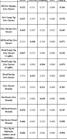
For the regression trees, the most important variables for predicting the response variables were site identification, sampling date, and material (Table 2). Replicate reef

assignment, A or B, rarely appeared as the basis of splits. Mean (µ) and standard deviation (SD) for the groupings within regression trees are presented as µ±SD.

Table 2. Summary of contributions of predictor variables to the overall R2 value for live oyster and sponge regression trees. Bolded terms indicate the highest relative contribution among predictors for the tree (column) of interest.

SiteID Material Sampling Reef Total R2 All Live Sponge,

Live Oyster 0.532 0.311 0.157 0.000 0.766 Live Large Sp,

Live Oyster 0.537 0.307 0.156 0.000 0.770 Live Sm Sp, Live

Osyter 0.419 0.307 0.242 0.032 0.245 All Dead Sp, Live

Oyster 0.214 0.448 0.338 0.000 0.571 Dead Large Sp,

Live Oyster (3 splits)

0.827 0.173 0.000 0.000 0.236 Dead Large Sp,

Live Oyster (5 splits)

0.406 0.090 0.504 0.000 0.479

Dead Sm Sp,

Live Oyster 0.274 0.433 0.293 0.000 0.515 Live Oyster

Density 0.470 0.019 0.511 0.000 0.701 Sm Oyster Live

Density 0.370 0.000 0.630 0.000 0.636 All Dead Oyster

Density 0.670 0.320 0.010 0.000 0.747 Sm Oyster Dead

Density 0.446 0.045 0.510 0.000 0.590 Live Sp on

Substrate (surface areal

coverage)

19

The regression tree of live oyster densities (oysters per m2 of substrate surface area) (Figure 2, R2 = 0.701) revealed sampling date and site as the greatest explanatory variables for live oyster densities among the 6 splits. Substrate type was the basis of only one split: NoR2 in the first 3 samplings, granite reefs (744±203) supported greater densities than the other reef foundation materials (352±133). NoR2 also showed the greatest overall live oyster densities (868±875) compared to the grouping of the other sampled sites (205±242). For the NoR2 group, samples collected in December 2016 (2124±781) separated from the earlier sampling dates (450 ±229). Among the other sites (not NoR2), NoR1, NpR2, NpR4, and NpR5 (338±299) had greater densities of live oyster than the reefs on NoR3, NoR4, NoR5, NpR1, and NpR3 (105±110). During the May 2014 and June 2015 sampling, NpR4 (366±181) had greater live oyster densities than NpR2, NpR5, and NoR1 (160±131). The regression tree groupings for the density of live oysters <40 mm (Figure 3), was similar to those for live oyster density, with the exception that substrate type was no longer the basis of any splits.

For the regression tree of dead oyster density (Figure 4, R2 = 0.747), site identification contributed most to the variability within groups followed by sampling data and substrate

20

Figure 2. Regression tree of live oyster density with 6 splits, means are representative of oysters per m2 of substrate surface area (R2 = 0.701).

21

When examining the dead oysters <40 mm, the analysis produced a regression tree, within which where sampling date and site identification contributed most to the divisions followed by substrate type (Figure 5, R2 = 0.590). When substrate type determined a split, concrete was generally the substrate with greatest dead oyster density. For the first three sampling dates, NpR4, NpR5, NoR4, and NoR5 had greater densities of small dead oysters (356±242) than the other sites (174±147). At sites 4 and 5 in both NpR and NoR, densities of dead oysters increased through time.

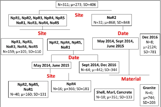
For the regression tree of mean percent surface area coverage of live boring sponge on cultch material (Figure 6, R2 _{= 0.904), site identification and substrate type explained a greater}

portion of the variability than the sampling date (60.6% and 35%, respectively). The first split in this tree was based on substrate material with shell cultch exhibiting greater percent cover by live sponge (34.6%±36.8%) than the other substrate types. Mid-estuary shell reefs of NoR3, NoR4, and NpR4 showed the greatest percent live sponge cover (83.8%±15.3%). On shell reefs at NpR2, NpR3, NpR5, and NoR2, greater coverage of the shell material was observed in May 2014 (36.8%±17.3%) than at the later 3 samplings (15.2%±14.6%). The non-carbonate reefs of granite and concrete (0%±0%) were distinct from the marl reefs (11.8%±20.0%). More sponge covered marl substrate at the mid-estuary sites of NoR3 and 4 and NpR4 (35.1%±21.8%) than other sites (1.2%±2.6%). Within the mid-estuary marl reef grouping, sponge coverage was greater in June 2015 and December 2016 samples (49.6%±15.2) than in the May 2014 and September 2014 samples (20.7%±17.4%).

For the regression tree of the proportion of live sponge (C. celata + non-C. celata spp.) within live oysters (Figure 7, R2 = 0.766) mid-estuary sites NpR4, NoR3, and NoR4

22

identification contributed the most to the variability of live sponge infestation followed by the reef material and sampling date. On reefs at NpR4, NoR3, and NoR4, oysters on the marl and shell reefs (0.602±0.293) were more heavily infested than the granite and concrete reefs

(0.154±0.231). Within the marl/shell grouping, the oysters collected at the May 2014 sampling (0.309±0.221) showed lower proportions of live sponge infestations than the later sampling dates (0.710±0.240). Within the granite/concrete grouping, the December 2016 sampling

(0.402±0.253) revealed higher proportions of live sponge infestation than the earlier sampling dates (0.074±0.157). The same tree structure was obtained analyzing the proportion of live

Cliona celata in live oysters (Appendix 2).

The regression tree that examined the proportion of live non-C. celata sponge within live oysters (Appendix 2, R2 = 0.245) had a low amount of variation explained by the dependent variables; thus, limiting biologically/ecologically relevant interpretations of the non-C. celata

sponge infestation proportions. However, within the NpR2 and NoR2 sites, granite and concrete reefs (0.0029±0.0092) had lower proportions of live non-C. celata sponge infestations than the shell and marl reefs (0.0381±0.081).

The regression tree of the proportion of dead sponge (C. celata + non-C. celata spp.) within live oysters (Figure 8, R2 = 0.236) revealed increased levels of dead sponge on shell reefs during the 2 sampling dates after the 2014 freshet at sites NpR2, NpR3, and NoR1

(0.294±0.200). Live oysters on shell reefs at NpR2, NpR3, NoR1, and NoR2 (0.182±0.196) had more dead sponge coverage than the live oysters on the granite, concrete, marl reefs

23

24

25

Figure 6. Regression tree of the average surface area coverage of live sponge on substrate material with 7 splits (R2 = 0.904).

N=311; μ=0.116; SD=0.252

Concrete, Granite, Marl

Material

Shell

Concrete,

Granite

N=156;

μ=0; SD=0

Marl

Material

NpR1, NpR2, NpR3, NpR5,

NoR1,NoR2, NoR5

N=53; μ=0.012; SD=0.026

NpR4,

NoR3,

NoR4

Site

May 2014,

Sept 2014

N=12;

μ=0.207;

SD=0.174

June 2015,

Dec 2016

N=12;

μ=0.496;

SD=0.152

Date

NpR1, NpR2, NpR3, NpR5,

NoR1, NoR2, NoR5

NpR4,

NoR3, NoR4

N=24;

μ=0.838;

SD=0.153

Site

NoR1, NpR1,

NpR5

N=22; μ=0.012;

SD=0.034

NoR2, NpR2,

NpR3, NpR5

Site

Sept 2014, June

2015, Dec 2016

N=24; μ=0.152;

SD=0.146

May 2014

N=8;

μ=0.368;

SD=0.173

26

Figure 7. Regression Tree of the proportion of any live sponge covering live oysters with 4 splits (R2_{= 0.766).}

The proportion of dead non-C. celata sponge that covered live oysters (Figure 9, R2 = 0.515), was greatest at NoR1, NoR2, NpR2, and NpR3 (0.053±0.108) especially on shell reefs at the September 2014 and June 2015 samplings (0.235±0.180). For this tree, substrate type

explained the greatest portion of variability followed by sampling date and site identification. The same response variables were used to analyze relationships for dead oysters; (= left attached valves and boxes). These results are not included in this report. Overall, the structures of the trees of dead oyster demographics were similar to those for the live oyster regression trees.

27

Figure 8. Regression Tree of the proportion of any dead sponge cover on live oysters with 3 splits (R2 = 0.571).

28

Cause of Death

A chi-squared multiple comparisons for both the North River and Newport River box mortality data acquired in September 2014 revealed that cause of death varied significantly with site (Χ2_{= 18.442, df = 8, p = 0.02 and Χ}2_{= 77.902, df = 8, p = 1.3e-13, respectively). In general,}

deaths attributed to boring sponge (boxes filled with live sponge tissue) were most common at sites 3 and 4 in both NoR and NpR. In both systems, drill kills were found at sites 3, 4, and 5. In the North River, the greatest proportions of drill kills were at NoR3. In contrast, NpR5 was the site of the greatest proportions of drill-killed boxes. Boxes with evidence of death caused by a crushing predator were less common in the North River than in the Newport River, though these occurred in relatively low numbers overall. Similar trends were observed for the June 2015 and December 2016 sampling events and are displayed in Appendix 3. For the North River, causes of death revealed by boxes varied significantly with location in both June 2015 (Χ2= 37.586, df = 12, p = 1.8e-4) and December 2016 (Χ2_{= 230.43, df = 12, p = 2.2e-16). Cause of death also}

29

30

DISCUSSION

Dunn et al. (2014) reported on live oyster demographics on our experimental reefs over the first 12 months post-deployment, noting only minor initial differences in oyster recruitment among the four substrate types used as reef foundations. At the 12-month sampling, Dunn et al. (2014) found no distinct advantage or disadvantage of substrate choice on overall reef

performance. Our longer-term monitoring, up to 54 months post-construction, revealed distinct advantages of non-carbonate substrates at some sites by delaying boring sponge infestations within developing oyster communities.

The upper portions of both the Newport River and North River estuaries showed strong evidence of freshet influence, revealed primarily by boring sponge mortality observed on these reefs in the September 2014 sampling, roughly 1 month after the summer 2014 freshet subsided (see Figures 8, 9). Observable down-estuary influences of the 2014 freshet on boring sponge populations did not extend below NpR2 and NoR2 in the Newport River and North Rivers, respectively. In the Newport River, this freshet could have affected the Clionid sponges at NpR3, but this remains uncertain due to the soft flocculent mud at this site, which periodically covers portions of the reefs. Given that in December 2016, a small amount of live boring sponge was found on NpR2 (see NpR2 LFDs, Appendix 1) and there were only empty galleries in shells NpR3 (see NpR3 LFDs, Appendix 1), periodic burial/partial burial of the NpR3 reefs by soft, shifting mud could be a major source of sponge mortality. These data suggest that the summer freshets of 2014 and 2015 in the Newport River and North River were not as severe as

31

1947) and 1955 (Wells 1959, 1961) in the Newport and North Rivers. In his study of boring sponge populations in the Newport River, Wells (1961) reported freshets killing boring sponges at Piver’s Island, a station ~10km down-estuary of NpR3 and roughly equivalent to the position of NpR5.

Over the 54 months of observation, the mid-estuary sites in the North River estuary (NoR3 and NoR4) never produced high densities of adult oysters on reefs of any substrate type (Figure 2). Oysters that recruited to all substrates at these sites appeared to be killed at the early juvenile stages by the combination of predation and boring sponge infestation, effectively

creating a population bottleneck for oyster reefs in this portion of the North River estuary (Figure 7). These results indicate that it is inadvisable to construct subtidal oyster reefs of any substrate type at these locations. Historical surveys of the North River indicate subtidal oyster reefs did not occur in the vicinity of NoR4 in the late 19th and early 20th centuries (Winslow 1889 and Grave 1904, respectively). Rather, the bottom of this region of the estuary was characterized as firm mud where large single oysters and small clusters of oysters would grow partially buried in the sediment with only a small portion of their distal shell margin exposed above the sediment. Being mostly buried, the oysters largely escaped predation and colonization by boring sponges. Because historically oyster reefs did not exist in the mid-portions of the estuary, dense

populations of relatively immobile oyster predators, like oyster drills, likely did not occur within the mid-estuary portions of the North River.

32

the granite and concrete substrates (Figure 6), the recruitment of boring sponge to live oysters on these substrates must have originated via sponge larval recruitment. The boring sponge could then subsequently spread to neighboring oysters if in direct contact with an infested oyster; however, boring sponge infestation of oysters on granite and concrete reefs do not originate from the substrate. The rate of oyster infestation by boring sponge on the granite and concrete reefs provides a baseline rate for the sponge infestation via larval recruitment. The rapid rates of boring sponge infestation of oysters occupying carbonate substrates, particularly oyster shell, are likely driven by rapid contact spread of boring sponge through the substrate bed and then into attached oysters.

Existing (Carver et al. 2010) and new knowledge generated by this study regarding mechanisms of boring sponge recruitment and spread into oyster reef habitats and the importance of reef materials should be incorporated into current strategies oyster habitat restoration and estuarine development projects in general. Whether intended for oyster habitat creation (oyster fishery enhancement and no-take oyster reserves), as well as for submerged structures like jetties, groins, breakwaters, and artificial reefs for fish enhancements, substrate type must be carefully considered for its impacts on the estuarine ecosystem in genereal. For example, the use of marl for jetty construction in proximity to inlets (e.g. Radio Island Jetty Morehead City, NC) provides exceptionally favorable habitat for boring sponge populations, thereby negatively influencing surrounding oyster habitats.

33

to be infested with boring sponge - from the reefs to retard the development of the boring sponge community. With the periodic removal of larger oysters, as well as culling out sponge-infested shell materials, the newly exposed reef materials returned to the reef bed should be available for new oyster recruits without being in direct contact with sponge-infested substrates. It is unlikely this strategy would work for reefs with carbonate-based foundations that become heavily infested with boring sponges. Thus, carbonate materials should not be used in regions of the estuary where boring sponges flourish.

If carbonate material is allowed to remain in the subtidal environment where boring sponges thrive (e.g. NpR4, NoR3 and NoR4), the carbonate may become mechanically and/or chemically eroded to the point of functional disappearance. If the recruitment of new oysters to a fading carbonate foundation is weak, the addition of new carbonate materials to the system is cut-off, further reducing exposed surfaces for new oyster recruitment onto the reef (Soniat et al. 2014, Waldbusser et al. 2013). Evidence of this aging out of a reef underpinned by a carbonate material can be found in the Newport River near the NpR3 reef sites. In this area, patches of subtidal reefs have succumbed to harvest pressure, predation pressure, and boring sponges to the point of becoming a bottom type called “crush” by oystermen (A. Tyler, pers. comm.). Crush consists of heavily degraded shells, often broken into pieces that sit just below the surface of soft muds. Areas of exposed “crush” that we examined in the Newport River did not support live oyster populations. Rather the “crush” was often heavily infested by boring sponge – live if exposed and dead if buried (G. Sorg, pers. obs).

34

for additional oyster recruitment. If the boring sponges do not enter the gamma stage due to consumptive pressure (Guida 1976), a reef with non-carbonate foundations may exhibit an oyster “boom and bust” on multi-year to decadal timescales. Because the experimental reefs of this study have only been deployed for 54 months (as of December 2016), we have not had the opportunity to observe this hypothesized growth and collapse of both oysters and sponges on the reefs at NpR4. The “boom and bust” cycle did not occur at NoR3 and NoR4 because the initial bottleneck induced by intense boring sponge and predation pressures prevented an initial “boom”.

Data from our long-term study strongly suggest that the subtidal oyster reefs at our highest salinity sites in the Newport River and North River estuaries (NpR5 and NoR5, respectively) reside within an estuarine salinity zone that cannot sustain subtidal oyster

populations because of intense predation and other pest pressures (Figure 10). Further, at NoR5, sand transport hampered subtidal reef development by periodically covering all or portions of most reefs created at this site. Data on sources of oyster mortality from NpR5 boxes

demonstrated enormous top-down controls on oyster populations, most notably from oyster drills. At this site, predation by drills on juvenile oysters represents a substantial population bottleneck.

We also found evidence of oyster drills feeding on small size-classes at the NpR3 and NpR4, but at substantially lower levels (Figure 10) than at NpR5. Drill kills were also numerous at NoR3 and NoR4. Wells (1961) reported that during his study in 1955-1956, the upper

35

of the freshet. This suggests that the modern Newport River estuary may be substantially saltier and/or the salinity is much less variable than during Wells’ experimental period.

Salinity tolerance is often cited as a basic driver of species distributions in estuarine systems (Wells 1961, Crain et al. 2004, Galván et al. 2016 and references therein). In estuaries, mean salinity is not the only salinity parameter affecting species distributions. Deviations from a site’s mean salinity value may be more important than the mean salinity value (La Peyre et al. 2009), and in particular freshets, which cause major and often sustained drops in salinity. Large and long-lasting freshets occur naturally from sustained heavy rainfall and can persist for days or weeks (de Laubenfels 1947, Wells 1959, 1961) or via manmade water diversions (La Peyre et al. 2009). Freshet duration and frequency likely play a central role in purging the upper estuarine environment of marine adapted oyster pest species such as boring sponges, oyster drills, and

Stylocus spp. flatworms (Wells 1959, 1961).

36

2012, NC DMF only planted cultch above the causeway once in 2010 and at a single site. This particular cultch planting was close (~200 m) to the failed NoR3 reefs.

Winner’s (2015) study also compared the condition of this above the causeway 2010 cultch planting in the North River with that of a relic oyster reef buried by ~15-20 cm of muddy sediments below the cultch shell. By 2015, the initial dense oyster communities on this cultch planting collapsed and the cultch shell, hash, and few remaining live oysters on this site were heavily infested by C. celata. In stark contrast, the relic reef revealed a vibrant oyster

community composed of multiple size classes and hosting a low level of non-C. celata boring sponges, which are more adapted to low salinity environments (Hopkins 1956), and showed little evidence of C. celata boring sponge. This contrast in the boring sponge assemblages of the relic reef and cultch planting indicate that since the 1899 surveys by Grave (1904), when this relic reef appeared to be exposed, there has been a substantial shift toward a saltier salinity regime in the upper North River estuary.

Beginning in 1911, Beaufort Inlet, the site of seawater exchange for both the Newport and North River estuaries, has been mechanically dredged to create shipping channels leading to the Port of Morehead City. The channel dredging of Beaufort Inlet has been correlated with an increased tidal amplitude in the vicinity of Beaufort, NC (Zervas 2003, van Maren 2015), likely contributing to increased saltwater penetration into the North and Newport River estuaries. The recently developed SalWise salinity database reveals an increase in salinity since 1945 based on historical salinity records for the Newport River and North River estuary regions (Lindquist and Fegley 2016).

37

pests, as does this modern-day study. In the North River, he concluded that no attempts to establish oyster beds for commercial oyster harvest, on public or leased bottom, should occur down-estuary from a line extending from just above Ward’s Creek running W/NW toward the west side of the North River (Figure 11). Results of our multiple substrate comparisons across the salinity gradient in the North River indicates that the Grave’s line has migrated ~4km upstream in the present North River estuary near NoR2, a region known locally as “The

Narrows”. In the Newport River, Grave drew the favorable/unfavorable habitat line for oysters from a point on the north shore of the estuary just to the east of Harlowe Creek running S/SW to the south shore near Crab Point (Figure 12) Our project data would shift Grave’s line ~1.5km up-estuary in the modern Newport River estuary, bisecting the estuary in roughly NW-SE orientation between NpR2 and NpR3. Below these lines, our data indicate biological stresses associated with predation, boring sponges, and other oyster pests are too intense to support viable subtidal oyster populations. It is informative to note that areas below Grave’s 1904 lines in the late 19th _{and early 20}th _{centuries did not host natural subtidal oyster reefs (Winslow 1889, Grave}

1904), yet in the early 20th century, shellfish leases for oyster production were commonly sited below his lines. The vast majority of oyster culturing attempts failed and were abandoned (Grave 1904).

38

Figure 11. Upper North River estuary study site locations with Grave’s (1904) line (green) for lower limits of regions for subtidal oyster reef construction and the redrawn line (red) from the results of this study. The dashed line indicates the location of the NC DMF 2016-2017

39

Figure 12. Upper Newport River estuary study site locations with Grave’s (1904) line (green) for lower limits of regions for subtidal oyster reef construction and the redrawn line (red) from the results of this study. The dashed line indicates the location of the NC DMF 2016-2017 permanent closure line for oyster harvesting.

40

low levels. Further, large geographic barriers between up-estuary subtidal oyster populations and more down-estuary pest populations created by large freshet disturbances may now be bridged more quickly by oyster pests via the created “stepping stone” reefs.

We have observed that oyster communities at upper-estuary sites in both the Newport and North River systems are characterized by variable recruitment but high survival. The highest salinity sites in both estuaries consistently saw high numbers of oyster larvae settling on substrates, regardless of substrate type; however, this high settlement is negated by intense predation pressure. At mid-estuary sites in the North River estuary, boring sponges and other oyster pests prevent juvenile oyster survival on all substrates. In the Newport River estuary, the mid-estuary site NpR4 was characterized by high incidences of live boring sponge on live and dead oysters and on reef foundation oyster shells and marl, while the rates of boring sponge colonization of live and dead oysters on the non-carbonate materials were delayed until the 54-month sampling. At upper-estuary sites with lower salinities and large freshet influences, boring levels were low to none. In these regions, the level of obvious shell damage from Polydora spp.

polychaetes rise considerably; however, no rigorous data were collected regarding Polydora

impacts on oysters. Importantly, the freshets occurring during the first 54 months of this study did not curtail boring sponge populations in mid- and lower-estuary portions of the Newport River as did the freshets in the early 20th century.

41

materials and the oysters occurring on them are highly susceptible to boring sponge colonization in mid and lower portions of estuaries. Carbonate materials should not be used for oyster

APPENDIX 1: LENGTH FREQUENCY DISTRIBUTIONS FOR NORTH AND NEWPORT RIVER ESTUARIES

43

_{Live Oyster}

_{Dead Oyster}

_{Live Sponge}

_{Dead Sponge}

North River Site 1: September 2014 Sampling

Oyster Length (mm) Oyster Length (mm)

0 5 10 15 20 25 30

0 20 40 60 80 100 120 0 5 10 15 20 25 30

0 20 40 60 80 100 120

Granite

0 20 40 60 80 100 120 0

5 10 15 20 25 30

0 20 40 60 80 100 120

Shell

0 20 40 60 80 100 120 0

5 10 15 20 25 30

0 20 40 60 80 100 120

Marl

0 20 40 60 80 100 120 0 5 10 15 20 25 30

0 20 40 60 80 100 120

44 0 5 10 15 20 25 30

0 20 40 60 80 100 120 0 5 10 15 20 25 30

0 20 40 60 80 100 120

0 5 10 15 20 25 30

0 20 40 60 80 100 120

0 5 10 15 20 25 30

0 20 40 60 80 100 120 0 5 10 15 20 25 30

0 20 40 60 80 100 120

0 5 10 15 20 25 30

0 20 40 60 80 100 120

0 5 10 15 20 25 30

0 20 40 60 80 100 120

0 5 10 15 20 25 30

0 20 40 60 80 100 120

Live Oyster

Dead Oyster

Live Sponge

Dead Sponge

North River Site 1: June 2015 Sampling

Oyster Length (mm) Oyster Length (mm)

45 0 5 10 15 20 25 30

0 20 40 60 80 100 120 0 5 10 15 20 25 30

0 20 40 60 80 100 120 0

5 10 15 20 25 30

0 20 40 60 80 100 120

0 5 10 15 20 25 30

0 20 40 60 80 100 120 0 5 10 15 20 25 30

0 20 40 60 80 100 120 0 5 10 15 20 25 30

0 20 40 60 80 100 120 0

5 10 15 20 25 30

0 20 40 60 80 100 120

0 5 10 15 20 25 30 35 40

0 20 40 60 80 100 120

Live Oyster

Dead Oyster

Live Sponge

Dead Sponge

North River Site 1: December 2016 Sampling

Oyster Length (mm) Oyster Length (mm)

46

_{Live Oyster}

_{Dead Oyster}

_{Live Sponge}

_{Dead Sponge}

North River Site 2: May 2014 Sampling

Oyster Length (mm) Oyster Length (mm)

0 5 10 15 20 25 30

0 20 40 60 80 100 120 0 5 10 15 20 25 30

0 20 40 60 80 100 120

Granite

0 20 40 60 80 100 120 0

5 10 15 20 25 30

0 20 40 60 80 100 120

Shell

0 20 40 60 80 100 120 0

5 10 15 20 25 30

0 20 40 60 80 100 120

Marl

0 20 40 60 80 100 120 0 5 10 15 20 25 30

0 20 40 60 80 100 120

47

_{Live Oyster}

_{Dead Oyster}

_{Live Sponge}

_{Dead Sponge}

North River Site 2: September 2014 Sampling

Oyster Length (mm) Oyster Length (mm)

0 5 10 15 20 25 30

0 20 40 60 80 100 120 0 5 10 15 20 25 30

0 20 40 60 80 100 120

Granite

0 20 40 60 80 100 120 0

5 10 15 20 25 30

0 20 40 60 80 100 120

Shell

0 20 40 60 80 100 120 0

5 10 15 20 25 30

0 20 40 60 80 100 120

Marl

0 20 40 60 80 100 120 0 10 20 30 40 50

0 20 40 60 80 100 120

48 0 5 10 15 20 25 30

0 20 40 60 80 100 120 0 5 10 15 20 25 30

0 20 40 60 80 100 120

0 5 10 15 20 25 30

0 20 40 60 80 100 120

0 5 10 15 20 25 30

0 20 40 60 80 100 120 0 5 10 15 20 25 30

0 20 40 60 80 100 120

0 5 10 15 20 25 30

0 20 40 60 80 100 120

0 5 10 15 20 25 30

0 20 40 60 80 100 120

0 5 10 15 20 25 30

0 20 40 60 80 100 120

Live Oyster

Dead Oyster

Live Sponge

Dead Sponge

North River Site 2: June 2015 Sampling

Oyster Length (mm) Oyster Length (mm)

49 0 20 40 60 80 100

0 20 40 60 80 100 120 0 20 40 60 80 100

0 20 40 60 80 100 120

Live Oyster

Dead Oyster

Live Sponge

Dead Sponge

North River Site 2: December 2016 Sampling

Oyster Length (mm) Oyster Length (mm)

Granite

Shell

Marl

Concrete

0 20 40 60 80 100 120

0 20 40 60 80 100

0 20 40 60 80 100 120 0 20 40 60 80 100

0 20 40 60 80 100 120 0 20 40 60 80 100

0 20 40 60 80 100 120 0

20 40 60 80 100

0 20 40 60 80 100 120

0 20 40 60 80 100

50

_{Live Oyster}

_{Dead Oyster}

_{Live Sponge}

_{Dead Sponge}

North River Site 3: May 2014 Sampling

Oyster Length (mm) Oyster Length (mm)

0 5 10 15 20 25 30

0 20 40 60 80 100 120 0 5 10 15 20 25 30

0 20 40 60 80 100 120

Granite

0 20 40 60 80 100 120 0

5 10 15 20 25 30

0 20 40 60 80 100 120

Shell

0 20 40 60 80 100 120 0

5 10 15 20 25 30

0 20 40 60 80 100 120

Marl

0 20 40 60 80 100 120 0 5 10 15 20 25 30

0 20 40 60 80 100 120

51

_{Live Oyster}

_{Dead Oyster}

_{Live Sponge}

_{Dead Sponge}

North River Site 3: September 2014 Sampling

Oyster Length (mm) Oyster Length (mm)

0 5 10 15 20 25 30

0 20 40 60 80 100 120 0

5 10 15 20 25 30

0 20 40 60 80 100 120

Shell

0 20 40 60 80 100 120 0

5 10 15 20 25 30

0 20 40 60 80 100 120

Marl

0 20 40 60 80 100 120 0 5 10 15 20 25 30

0 20 40 60 80 100 120

Concrete

0 20 40 60 80 100 120 0 10 20 30 40 50 60

0 20 40 60 80 100 120

52

_{Live Oyster}

_{Dead Oyster}

_{Live Sponge}

_{Dead Sponge}

North River Site 3: June 2015 Sampling

Granite

Shell

Marl

Concrete

0 20 40 60 80 100 120 0 5 10 15 20 25 30

0 20 40 60 80 100 120 0

5 10 15 20 25 30

0 20 40 60 80 100 120

0 5 10 15 20 25 30

0 20 40 60 80 100 120 0 5 10 15 20 25 30

0 20 40 60 80 100 120 0 5 10 15 20 25 30

0 20 40 60 80 100 120 0

5 10 15 20 25 30

0 20 40 60 80 100 120

0 5 10 15 20 25 30

0 20 40 60 80 100 120

Oyster Length (mm) Oyster Length (mm)

53 0 5 10 15 20 25 30

0 20 40 60 80 100 120 0 5 10 15 20 25 30 35 40

0 20 40 60 80 100 120 0

5 10 15 20 25 30 35 40

0 20 40 60 80 100 120

0 5 10 15 20 25 30

0 20 40 60 80 100 120 0 5 10 15 20 25 30

0 20 40 60 80 100 120 0 5 10 15 20 25 30

0 20 40 60 80 100 120 0

5 10 15 20 25 30

0 20 40 60 80 100 120

0 5 10 15 20 25 30

0 20 40 60 80 100 120

Live Oyster

Dead Oyster

Live Sponge

Dead Sponge

North River Site 3: December 2016 Sampling

Oyster Length (mm) Oyster Length (mm)

54

_{Live Oyster}

_{Dead Oyster}

_{Live Sponge}

_{Dead Sponge}

North River Site 4: May 2014 Sampling

Oyster Length (mm) Oyster Length (mm)

0 5 10 15 20 25 30

0 20 40 60 80 100 120 0 5 10 15 20 25 30

0 20 40 60 80 100 120

Granite

0 20 40 60 80 100 120 0

5 10 15 20 25 30

0 20 40 60 80 100 120

Shell

0 20 40 60 80 100 120 0

5 10 15 20 25 30

0 20 40 60 80 100 120

Marl

0 20 40 60 80 100 120 0 5 10 15 20 25 30

0 20 40 60 80 100 120

55

_{Live Oyster}

_{Dead Oyster}

_{Live Sponge}

_{Dead Sponge}

North River Site 4: September 2014 Sampling

Oyster Length (mm) Oyster Length (mm)

0 5 10 15 20 25 30

0 20 40 60 80 100 120 0 5 10 15 20 25 30

0 20 40 60 80 100 120

Granite

0 20 40 60 80 100 120 0

5 10 15 20 25 30

0 20 40 60 80 100 120

Shell

0 20 40 60 80 100 120 0

5 10 15 20 25 30

0 20 40 60 80 100 120

Marl

0 20 40 60 80 100 120 0 10 20 30 40

0 20 40 60 80 100 120

56 0 5 10 15 20 25 30

0 20 40 60 80 100 120 0 10 20 30 40 50

0 20 40 60 80 100 120

0 5 10 15 20 25 30

0 20 40 60 80 100 120

0 5 10 15 20 25 30

0 20 40 60 80 100 120 0 5 10 15 20 25 30

0 20 40 60 80 100 120

0 5 10 15 20 25 30

0 20 40 60 80 100 120

0 5 10 15 20 25 30

0 20 40 60 80 100 120

0 5 10 15 20 25 30

0 20 40 60 80 100 120

Live Oyster

Dead Oyster

Live Sponge

Dead Sponge

North River Site 4: June 2015 Sampling

Oyster Length (mm) Oyster Length (mm)

57 0 20 40 60 80 100

0 20 40 60 80 100 120 0 5 10 15 20 25 30 35 40

0 20 40 60 80 100 120 0

5 10 15 20 25 30 35 40

0 20 40 60 80 100 120

0 5 10 15 20 25 30

0 20 40 60 80 100 120 0 5 10 15 20 25 30

0 20 40 60 80 100 120 0 5 10 15 20 25 30

0 20 40 60 80 100 120 0

5 10 15 20 25 30

0 20 40 60 80 100 120

0 5 10 15 20 25 30

0 20 40 60 80 100 120

Live Oyster

Dead Oyster

Live Sponge

Dead Sponge

North River Site 4: December 2016 Sampling

Oyster Length (mm) Oyster Length (mm)

58

_{Live Oyster}

_{Dead Oyster}

_{Live Sponge}

_{Dead Sponge}

North River Site 5: May 2014 Sampling

Oyster Length (mm) Oyster Length (mm)

0 5 10 15 20 25 30

0 20 40 60 80 100 120 0 5 10 15 20 25 30

0 20 40 60 80 100 120

Granite

0 20 40 60 80 100 120 0

5 10 15 20 25 30

0 20 40 60 80 100 120

Shell

0 20 40 60 80 100 120 0

5 10 15 20 25 30

0 20 40 60 80 100 120

Marl

0 20 40 60 80 100 120 0 5 10 15 20 25 30

0 20 40 60 80 100 120

59

_{Live Oyster}

_{Dead Oyster}

_{Live Sponge}

_{Dead Sponge}

North River Site 5: September 2014 Sampling

Oyster Length (mm) Oyster Length (mm)

0 5 10 15 20 25 30

0 20 40 60 80 100 120 0 10 20 30 40

0 20 40 60 80 100 120

Granite

0 20 40 60 80 100 120 0

10 20 30 40 50 60 70

0 20 40 60 80 100 120

Marl

0 20 40 60 80 100 120 0

10 20 30 40

0 20 40 60 80 100 120

Shell

0 20 40 60 80 100 120 0 10 20 30 40 50

0 20 40 60 80 100 120