An investigation of using a polynomial loglinear model to evaluate differences in test score distributions

An Investigation of Using a Polynomial Loglinear Model to Evaluate Differences in Test Score Distributions

Diane Talley

A thesis submitted to the faculty of the University of North Carolina at Chapel Hill in partial fulfillment of the requirements for the degree of Masters of Arts, Educational Psychology, Measurement, and Evaluation; School of Education

Chapel Hill 2009

Abstract

Diane Talley: An Investigation of Using a Polynomial Loglinear Model to Evaluate Differences in Test Score Distributions

(Under the direction of Gregory Cizek)

Acknowledgements

I am grateful to many people for helping me through this difficult and lengthy journey. A special thanks to Dr. Gregory Cizek for letting me continue this research under his guidance and for pushing me to do my best. We could have taken an easier road, but where is the satisfaction in that?

I also offer thanks to Dr. Rita O’Sullivan and Dr. William Ware for their willingness to remain on my committee, despite the extended time this has taken me to complete.

I am immeasurably grateful to Chris Weisen of the Odem Institude without whom I could not have taken on this particular study. His skills, which provided the program for conducting this study, and patience with what seemed like an endless process, are greatly appreciated.

To my husband, thank you for giving up a wintry home in Colorado near friends and family for the heat of North Carolina and the stress of life with a graduate student. Words cannot express how much the love and support have meant to me.

I am deeply grateful to my loving and nurturing mom for taking care of my family and me through two babies and this academic process. I recognize and sincerely

Table of Contents

List of Tables ... vii

List of Figures ... viii

Chapters I. Introduction………1

II. Review of Literature Constructing Multiple Forms of a Test ………..6

Equating………..9

Definitions and Properties………...9

Data Collection for Equating……….……12

Equating Methods………..17

Mean equating………17

Linear equating………..……….18

Equipercentile equating………..21

Equating with IRT………..24

Identity equating……….25

Determining Whether to Equate Forms……….26

Dorans and Lawrence Method………27

Assessing Equating Error………28

III. Methodology .……….37

IV. Results……….41

V. Conclusions and Discussion……….44

Appendix ………70

List of Tables

Table

1. Data Collection Designs………..………54

2. Mean-Squared Equating Error………..………..55 3. Polynomial Loglinear Model………..56 4. Descriptive Statistics from Original Hanson Studies for all

Score Distribution Pairs (SDP1, SDP2, SDP3)………57 5. Summary of Results for the Polynomial Loglinear Model in

Determining Differences Between Score Distributions on Two

Forms………58 6. Summary of Standard Mean Differences (SMD)……….59 7. Descriptive Statistics from Simulation Study for all Score

List of Figures

Figure

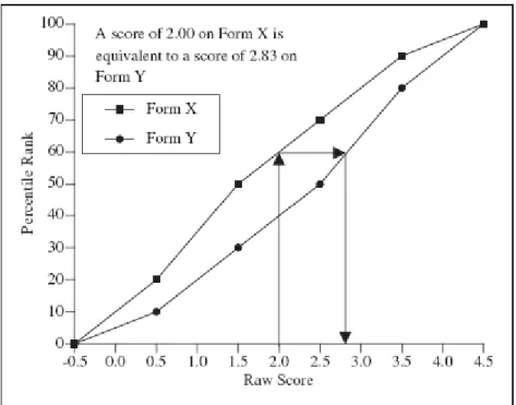
1. Example of Graphic Method of Equipercentile Equating………62

2. Score Distribution Pair 1 ……….………63

3. Form A-Score Distribution Pair 2………64

4. Form B-Score Distribution Pair………...65

5. Score Distribution Pair 3 ……….66

6. Process Methodology Flowchart………..67

7. Score Distribution Pair 1 (SDP1) from Simulated Data………..…68

8. Score Distribution Pair 2 (SDP2) from Simulated Data………..69

Ι. INTRODUCTION

Tests scores are used to inform important decisions that affect the public. Their impact may be on people in the school systems, people dependent on the quality of healthcare, or any number of other professional and educational fields where licensure or certification decisions are made. Industries such as health, education, legal, and government, and the people they service, depend on properly developed tests to ensure quality and safety. The process of developing examinations can be complex and subject to a wide range of challenges, from creating clear testing objectives to ensuring adequate resources

(financial and human) for the test development, administration, scoring, reporting and evaluation. At every step, validity evidence—that is, support for the inferences made from the results of the tests (Messick, 1989a), must be gathered and evaluated. If a test score is intended to reflect a certain level of proficiency in a given domain, there must be evidence to support that assertion.

One common problem in test development is the issue of basing decisions on data from small samples of examinees. If the data used to construct test forms come from a small sample of the intended population--especially if the sample is not truly representative of the target population- there may be weak or inadequate evidence to support the inferences made from the resulting scores. As Kane (2006) has noted: “The challenge is to make the

Jones, Smith, and Talley (2006) define as 0-200 examinees, but it can also be a consideration for large-scale programs when there are a limited number of examinees available for field-testing or other data analytic purposes. The data collected for test

development purposes are used to make important decisions regarding congruency of items to the content domain, item accuracy and statistical performance, item selection,

construction of test forms, scoring, and equating forms.

For a variety of reasons, testing programs may require multiple forms of a test that measure the same constructs. They may be necessary, for example, when tests are given at multiple times of the year, when a new form is used for each test administration, or when programs administer multiple forms concurrently. A testing program may need multiple forms to reduce item exposure for security purposes, or because failing examinees may be permitted to take a test multiple times. Clearly, a test is no longer a measure of the intended construct if a failing examinee is administered the same form on two occasions and will likely benefit from repeated exposure to the same items. With small-scale testing programs, item exposure may be less problematic than with larger programs. Fewer test takers see the items, but multiple forms may still be needed for repeat test takers and the issue of test security remains a concern.

test forms as well as sampling error. Specific ways of estimating the amount of error (e.g., standard error of equating) are addressed in more detail later in this section.

A primary goal in equating is to select data collection designs, sample sizes, and procedures that introduce the least amount of error. In some cases, the least error-prone equating procedure may be to do no equating at all, also referred to as identity equating (Kolen & Brennan, 2004). Sample size affects the amount of error introduced by equating. Other things being equal, the larger the sample size, the smaller the error of equating will be. When only small samples of data are available, it is important for test developers to consider the consequences of using a small sample size on the precision of the equating results. Peterson, Kolen, and Hoover (1989) stated “an approximate equating of scores on two forms of a test will generally be more equitable to the examinee than no equating at all, especially if the test forms differ in difficulty” (p. 243). However, it may be the case that even when test forms are developed to be parallel, the amount of error introduced in the equating process is greater than if no equating were done. According to Kolen and Brennan: “Only if equating is expected to add in less error than identity equating, should an equating other than identity equating be considered” (p. 296). Thus, when building tests that will be administered to small samples of examinees, sizes it is important to ask the question: Is the error introduced by equating greater than that associated with not equating at all?

introduced by Hanson (1992, 1996). Kolen and Brennan and Harris and Crouse (1993) recommended the approach introduced by Hanson when small samples are used to equate forms.

The method proposed by Hanson (1992, 1996) compares the score distributions on different forms of a given test to determine whether the samples likely come from the same population. If the distributions are evaluated to be equivalent, then the samples are

considered to be from the same population. In this case, no equating is recommended. If the distributions are found to be significantly different, then distributions are considered to be from different populations; thus, equating is necessary.

Although the Hanson method is recommended in the literature for small samples, Hanson (1996) indicated that this method might not, in fact, work well for small samples. When the sample sizes are very large, even a very small difference in distributions can be detected. Alternatively, the test may not be able to detect differences with a small sample size, even though there may be a significant enough difference between the distributions to warrant equating. As Hanson has recommended, “it is important that sample sizes be chosen so that meaningful differences in the distributions can be detected” (p. 319).

The purpose of the present study was to determine what sample size is needed for Hanson’s (1996) method to be able to detect meaningful differences between distributions. The study includes three pairs of distributions with varying mean differences to evaluate the power of Hanson’s method across varying sample sizes. A brief review of literature

II. REVIEW OF LITERATURE

The following review of literature is an examination of test construction and equating methodology, including relevant research as it pertains to developing multiple forms of a test using small samples of data. The review is followed by a discussion of the three methods for determining whether to equate forms: Dorans and Lawrence (1990), Assessing Equating Error, and the Hanson Method. An example of the Hanson method is provided for clarification.

Constructing Multiple Forms of a Test

The importance of proper test development procedures is critical to successful equating. Good test development begins with careful planning. This principle has been articulated by Mislevy who noted that:

Test construction and equating are inseparable. When they are applied in concert, equated scores from parallel test forms provide virtually exchangeable evidence about students’ behavior on the same general domain of tasks, under the same specified standardized conditions. When equating works, it is because of the way the tests are constructed (1992, p. 37).

and the interpretation of that measurement (Schmeiser & Welch, 2006). The content domain is the broadly defined area of the knowledge and skills to be tested. The test specifications define how that knowledge will be tested in a way that will support the interpretations of the resulting test scores. Test specifications provide specific information such as the number of forms to be developed, the number of items on each form, the intended testing audience, and test administration guidelines (Millman & Greene, 1989). In addition, test specifications may include a test blueprint, which dictates the number of items for each content area (Downing, 2006). A clear specification of what is being tested and why is critical to supporting the interpretations of the results; that is, validity (Kane, 2006).

When defining the parameters of the testing program, there should be an overall vision of what the program will look like, including its size. A very small program might consider creating only one form of a test, requiring simpler processes, fewer items, and statistical procedures that are more robust in the context of small sample sizes. Jones, Smith, and Talley (2006) recommend using a single form of a test for small testing programs, especially when there are little or no data available for test construction and equating. Where multiple forms are deemed necessary, special care should be taken in applying the steps of test development. Jones et al. suggest extra time and attention in the early phases of the test development process in an effort to minimize error in item and form construction, and to make forms as similar as possible before applying equating methods to the data.

same concepts in different ways” (p. 461). Item writing is a critical part of constructing similar forms. Item writers should be highly knowledgeable in the content area and trained on item writing techniques including how to write various item types (e.g., multiple choice, matching, constructed response), item writing rules (e.g., items should be clear and concise and avoid racial, gender, or other sources of potential bias), and writing items that are congruent with the content domain. Alignment of individual items on the test to the content domain is a primary source of validity evidence, showing the “relevance and

representativeness of the test content in relation to the content of the domain about which inferences are to be drawn and predictions made” (Messick, 1989b, p. 6). In addition to psychometric review, editorial review is conducted, and reviews by subject matter experts ensure the technical accuracy of the items.

Field testing is the next recommended step in the test development process (Millman & Greene, 1989; Schmeiser & Welch, 2006). Field testing is employed to assess the

Data from a field test can also be used to determine a score scale, which will then be used for equating scores. All subsequent forms are generally equated back to the original score scale (Kolen & Brennan, 2004). A score scale may simply be the raw score scale of an examination (e.g. 0-25 on a 25-item form), or it can be something more complex such as scaling using Item Response Theory (IRT) or some other transformation. For simplicity, the following discussion of equating will assume the use of a raw score scale.

The type of score scale and methods for scoring items should be defined in the test specifications (Millman & Greene, 1989; Schmeiser & Welch, 2006). The literature does not address at what point in the development process an equating plan should be made, but consideration for equating needs should be given at the beginning of the development process, especially if the data from the field test are going to be used for equating purposes. Equating requires the use of specific data collection designs, which will be addressed later in the discussion of equating.

Equating

Definition and Properties of Equating

As previously discussed, validity is the quality of the inferences drawn from the scores yielded by an examination. This means that if two forms of a test are developed to be equivalent, then the scores on those tests should mean the same thing. For example, if Examinee A scores 70 on Form X and Examinee B scores 70 on Form Y, then the

interpretation is that both examinees have the same level of knowledge, skill, or ability in the defined area. Is it accurate to say that the true scores for examinees A and B are the same on two different forms? It is accurate only if the two forms of the examination are identical or, if the scores on the two forms have been adjusted such that they are interchangeable.

There are four general assumptions or properties regarding equating: symmetry, same specifications, group invariance, and equity (Kolen & Brennan, 2004). The symmetry property states that conversion of scores from one form of the examination (X) to scores on a second form of the examination (Y) should be the same as the conversion of scores in the inverse (i.e., Y scores converted to X). This means that regression does not constitute an equating method (Kolen & Brennan 2004; Lord, 1980).

The same specifications property requires that all forms to be equated should be constructed to the same statistical and content specifications (Kolen & Brennan, 2004). Forms that cover even slightly different content can be linked or scaled for comparability, but not equated. Linking or scaling allows two forms to be associated with one another for comparison without making the scores on forms interchangeable.

As test results should be interpreted in the same way for all relevant groups of

requires that equating should not be affected by group membership. This is largely affected by the data collection design selected. These data collection designs for equating are discussed in detail in the following section.

The final property is the equity property. Lord (1980) stated that it should not matter to the examinees which form of the test is administered. For this property to be strictly true, forms would have to be parallel, which is impractical in practice. Thus, a more lenient version is accepted such that “examinees are expected to earn the same equated score on Form X as they would on Form Y” (Kolen & Brennan, 2004, p. 11). In addition to equated scores being the same, forms should be equally reliable (Holland & Dorans, 2006; Peterson et al., 1989; Wendel & Walker, 2006).

Reliability, like validity, pertains to the outcomes of the measurement rather than the instrument itself (Haertel, 2006). The desired result of a perfectly reliable measurement procedure is that if an examinee were to take the test repeatedly, under the same conditions and without any learning occurring between administrations, the outcome would always be the same. This is obviously not a realistic expectation and cannot be directly measured, but there are a number of ways to estimate the reliability of the results of a measurement.

Equal reliability is important to the equity property, because examinees may not be indifferent to which form is administered if the forms are not equally reliable. A more qualified examinee might want a more precise, reliable measure of abilities, and a less qualified examinee might prefer a less reliable measure that will have a higher error variance, increasing chances of passing (Petersen et al., 1989).

single group of examinees or they may be administered to two separate groups. The groups may be randomly selected and considered equivalent, or may be naturally occurring making it difficult to assume equivalency of groups. The following section describes these possible data collection designs when only small samples of examinees are available.

Data Collection for Equating

To equate two or more forms of an examination, test scores from a representative sample must be available. Before collecting these data, the structure of the testing program, the intended examinee population, and the available sample population should be

considered. The administration of the test affects data collection in that tests administered in testing windows may require different equating procedures than examinations that are administered on an ongoing basis. Examinees taking a test that is administered in a testing window must select from a limited number of days the test may be offered (e.g. April 1 or October 1). An examinee taking a test that is administered on an ongoing basis may be able to call up a testing center and take the test on any day he or she chooses.

Both the size of the available sample and the equivalency of examinees strongly impact which design to use. In accordance with the group invariance property of equating, samples used for equating forms should be unbiased and representative of the population of examinees defined for a particular test (Kolen & Brennan, 2004). Methods that use two groups for data collection must take into account group differences in ability. A description of the population sampled for data collection should always be documented, as it is the population to which the equating results will apply and will affect the interpretation of test scores and, ultimately, the validity of test score interpretations.

each that can assist in dealing with the restrictions of a particular testing program and reduce differences between sample(s) and the intended population. According to Kolen and

Brennan (2004), the three data collection designs are the random groups design, the single group design, and the common-item nonequivalent groups design. These designs and their variations are described and illustrated in Table 1.

The random groups design shown in Table 1 requires two samples to be drawn randomly from the population, creating two equivalent groups (or more if there are more than two forms). A check mark in the table indicates which sample from the population takes which form of the examination. For example, in Table 1, sample 1 from the population takes Form X, and sample 2 from the population takes Form Y. Two primary assumptions related to this design are that 1) the samples taken are sufficiently large, and 2) the forms are administered simultaneously. These assumptions make this design impractical for equating with small samples, or for programs that administer examinations in testing windows.

---Insert Table 1 about here.---

An issue that may affect the equating results when administering both examinations to a single group is an order effect (Kolen & Brennan, 2004; Wendel & Walker, 2006). Depending on the number of items in each form, examinees may become fatigued when taking the second form, lowering their scores on the second form. Also, it is possible that examinees might experience a learning effect from the first form, which might increase their scores on the second form. Either phenomenon can affect the reliability of scores resulting from the data collection. The single group design with counterbalancing, as shown in Table 1, may alleviate this problem.

The single group design with counterbalancing, also referred to as the

counterbalanced random-groups design in Petersen, Kolen, and Hoover (1989), and the counterbalanced design in Holland and Dorans (2006), requires that a single group be divided in two, with examinees randomly assigned to each group. The second group (P2 in Table 1) takes the tests in reverse order from the first group (P1), thus alleviating order effects.

If the forms of an examination are to be administered in testing windows or a field test conducted operationally, then the CINEG design shown in Table 1--also referred to as the nonequivalent groups with anchor test design (Holland & Dorans, 2006)--may be a more appropriate design. This design allows for equating using naturally occurring groups, as opposed to randomly selected groups, although naturally occurring groups may not be equivalent in ability. For example, in the case of an examination administered to one group of students in the spring and another group in the fall, these groups are not randomly selected or randomly assigned to a form of the examination and they may differ in average level of knowledge, skill, ability, experience, or some other relevant characteristic. Instead of using randomly selected groups to ensure similar abilities among examinees, a set of common items (also called an anchor test) is administered to both groups of examinees. Recall that equating deals with the differences in difficulty between forms and assumes that the examination will perform the same for all groups of examinees. The data from the common items provide a way to distinguish between differences in scores due to examinee ability and differences due to form difficulty, thus allowing the equating function to more precisely link scores between the two forms (Kolen & Brennan, 2004). Jones, Smith, and Talley (2006) stated that “when concurrent forms are to be constructed using classical test theory, the use of common items can ameliorate some of the effects of sampling error with small sample sizes by accounting for some of the random differences between groups of test takers” (p. 518).

distributed across all content domains. The common items should also perform in the same way. Ideally, items would be chosen that have similar statistical characteristics, such as average p-values and item-total correlations, indicating they are similar in difficulty and discrimination to the non-common items.

An anchor test can be internal or external to a test form. When anchor test items are internal, they should be placed in approximately the same locations on both forms (Kolen & Brennan, 2004). Internal anchor test items are typically scored, although there is no

requirement to do so. In an external anchor test, items are not usually scored and may be administered as a separate form. One of the disadvantages to using an external form is the effect of examinee motivation. If the examinees know the items in the anchor test are not scored they may not expend the same level of effort as well as they would on the operational examination, which could result in inaccurate equating.

The number of common items is also critical. Kolen and Brennan (2004)

recommended a number of items equal to or exceeding 20% of the total test length. A study conducted by Parshall, Du Bose-Houghton, and Kromrey (1995) indicated that greater overlap (as much as 69%) resulted in less equating error and bias than forms with less overlap (47%). Jones, Smith, and Talley (2006) recommended using the maximum number of common items without increasing security risks by overexposing items. The purpose of the anchor test is to provide as much information as possible about group ability without compromising the integrity of the examination.

to the process and may require that additional items be developed to accommodate this design. In addition, both the common groups design and the CINEG design may change the way field testing would be conducted if equating were not a consideration. Once data are collected, an appropriate equating method can be chosen. The data collection design will not affect which method to choose, but how that method is applied. The following section describes five equating methods and their viability for small sample situations.

Equating Methods

Equating can be performed using a number of different statistical techniques

including mean, linear, equipercentile, and IRT methods. The choice of method depends on the characteristics of the score distributions (shape of the distribution-linear or nonlinear- and dispersion of scores), the size of the available sample, and other considerations.

Mean Equating

Mean equating is the most basic equating method. It assumes that the score

distributions resulting from the administration of two test forms are the same except for the means (Kolen & Brennan, 2004). Thus, it is assumed that scores on the two forms will differ by the same amount at all score points. If there is a difference, for example, of one point for high scoring examinees, then there must also be a difference of one point between scores for middle scoring and low scoring examinees. This is an extremely limiting assumption, as it is rare that two test forms will result in distributions that differ systematically in this way across all score points. However, mean equating can be useful when scores only need to be equated at the cut score (the chosen passing score), and that cut score is at or near the mean.

) ( )

(X y Y

x−Μ = −Μ (1)

Solving for y:

) ( )

(X Y

x

y= −Μ +Μ (2)

where x is a score on Form X, M(X) is the mean of scores on Form X, M(Y) is the mean of scores on form Y, and y is a score on Form X transformed to a score on Form Y. For

example, if the mean of Form X is 50 and the mean of Form Y is 54, using equation 2: y = x – 50 + 54

= x + 4

then a score of 52 on Form X would be equivalent to a score of 51 on Form Y.

Accordingly, it is assumed that Form Y is four points easier than Form X at every point along the score scale. If this assumption holds, or when it is possible to equate only at or near the mean, mean equating is a good option for small sample testing situations (Jones et al, 2006).

Linear Equating

Linear equating is also useful for small sample testing situations. However, like mean equating, it has strong assumptions about the characteristics of the parent

students but easier for high achieving examinees, while Form Y may be easier for low achieving examinees and harder for high achieving examinees (Kolen & Brennan, 2004).

In a random groups data collection design, where a large sample is used and groups taking Form X and Form Y are assumed to be equivalent, a basic linear transformation that allows scores with the same deviation from the mean to be equal (Kolen & Brennan, 2004) can be used for equating:

) ( ) ( ) ( ) ( Y Y y X X x σ σ Μ − = Μ − (3)

Solving for y:

)] ( ) ( ) ( ) ( [ ) ( ) ( ) ( ) ( X X Y Y x X Y y x

l_y = = + Μ − Μ

σ σ σ

σ

(4)

where ly(x)is the linear conversion of a Form X score to a Form Y score,

) ( ) ( X Y σ σ is the

slope of the line, and ( )] ) ( ) ( ) ( [ X X Y

Y − Μ

Μ

σ σ

is the intercept. For example, if Form X has a

mean of 72 and a standard deviation of 10, and Form Y has a mean of 77 and standard deviation of 9, a Form X score of 75 would be equivalent to a Form Y score of 79.7 (Kolen & Brennan, 2004):

7 . 79 ) 72 ( 10 9 77 ) 75 ( 10 9 ) 75 ( = + − = y l

In this example, Form Y is 4.7 points easier than Form X at a Form X score of 75. On the same two forms, a score of 85 on Form X would transform to a score of 88.7 on Form Y, indicating Form Y is only 3.7 points easier than Form X for these higher-achieving examinees.

collection design, which, as discussed earlier, may not be suitable for small sample testing situations. The same formula would be used for a single groups design assuming there are no order affects.

Applying linear equating to a CINEG design requires the use of an anchor test to determine group differences. Correlations are used to compare group performance on the anchor test, which allows differences in group ability to be separated out from variations in form difficulty.

Regardless of the design used, sample size has a direct impact on the accuracy of linear equating, although there is no definitive sample size necessary for linear equating to be considered a sufficiently precise equating method. Tsai (1997) conducted a study that examined methods for determining sample sizes needed for mean, linear, and equipercentile equating. A minimum sample size was calculated where the error introduced by equating would not exceed the error expected when using no equating. The study used a linear equating method to equate scores to a base Form Y. When equating scores on Form X to Form Y, a minimum sample size of 32 was needed, and when equating a third form (Z) to the base Form Y the minimum sample size was 99 (Z) . Kolen and Whitney (1982) recommended linear equating in their study for a sample size of 200 compared to three-parameter IRT and Rasch models, and equipercentile equating.

better served by setting a cut score near the mean--assuming that a cut score in that location accomplishes the intent of the standard setting--and equating only near that cut score when possible (Jones et al., 2006; Kolen & Brennan, 2004). If equating is really necessary all along the score scale and distributions between forms are not linearly related, equipercentile equating would be the next logical choice to consider.

Equipercentile Equating

As distributions of scores are rarely perfectly linearly related, equipercentile equating can provide a more versatile equating method than mean or linear equating. It allows the score distributions on two forms to vary in the first four moments of the distribution (i.e., mean, standard deviation, skewness, and kurtosis). Mean and linear equating functions assume that scores differ by a constant (mean in mean equating, and mean and standard deviation in linear equating). In reality, scores may vary differently at different points on the score scale. Thus, equipercentile equating is more practical if scores need to be equated all along the score scale, rather than only at or near the mean.

in the example, a vertical line is drawn from the raw score 2.00 on the x-axis to the cumulative frequency distribution for Form X. A horizontal line is then drawn from that point to the cumulative frequency distribution for Form Y (this line corresponds to a particularcommon percentile rank, in this case about 60th). Finally, a vertical line is drawn from that point back to the x-axis to find the raw score equivalent on Form Y for the given score on From X which, in this case, is approximately 2.8.

---Insert Figure 1 about here.---

In the example shown in Figure 1, there is a limited score range (-0.5- 4.5). In reality, score ranges may be much larger, and the graphical method lacks some precision in deriving strictly equivalent scores. An analytical method is probably more practical and results in a more precise solution. The analytical method uses the function:

)]} 1 * ( *) ( )][ 5 . * ( [ ) 1 * ( { 100 )

(x = F x − + x− x − F x −F x −

P (5)

where P(x) is the percentile rank function, F is the cumulative distribution function, and x* is the discrete score closest to the actual score.

While equipercentile equating has less stringent assumptions about the shapes of the score distributions on forms, it is problematic for small-scale testing, as it requires larger sample sizes. The equipercentile equating function “compresses and stretches the score units on one test so that its raw score distribution coincides with that on the other test” making it very “data dependent” (Cook & Petersen, 1987, p 226). Sampling error is large when scores not achieved in a small sample cause irregularities in the distribution. This problem can be addressed by applying smoothing methods.

does so by estimating a smooth population distribution and replacing the observed scores with the estimated smoothed distribution. Smoothing may be done prior to equating (presmoothing) or after equating (postsmoothing). The importance of this method in the current discussion is that smoothing may make equipercentile equating more feasible for small sample sizes since it can reduce sampling error.

Livingston (1993) conducted a study to determine whether using loglinear smoothing could reduce sample sizes needed for equipercentile equating. Loglinear smoothing is a presmoothing technique that tries to fit the best model to the data by

estimating moments in the distribution. Sample sizes of 25, 50, 100, and 200 were tested in the context of a CINEG design. The smaller the sample size, the larger the reduction in error was. In all sample sizes tested, it was determined that equating with loglinear smoothing was preferred to not equating at all. Hanson, Zeng, and Colton (1994) also found that smoothing methods applied to sample sizes as small as 100 could provide more accurate equating results than equipercentile without smoothing and, in some cases, mean and linear equating.

Livingston suggested that the use of presmoothing may reduce the sample size needed for equipercentile equating by half, making it a more realistic choice for small-scale testing situations where scores need to be equated all along the score scale. However, even with the improved precision achieved with the use of smoothing, some of the more recent literature still does not recommend equipercentile equating for small sample sizes,

What constitutes an adequate sample size for equipercentile equating, with or without smoothing, is not definitive. Hanson, Zeng, and Colton (1994) suggested a sample size of 1000 for using equipercentile equating with presmoothing. Jarjoura and Kolen (1985) indicated the need for a large sample size (800) when using equipercentile equating. Jones, Smith and Talley (2006) recommended a minimum sample size of 628 with a standard error of equating of 1.0 and equating at the cut score when the cut score is near the mean; when the cut score is at least two standard deviations from the mean, the recommended sample size increased to 3056. In all of these studies, a random groups design was used with the exception of the Jarjoura and Kolen study, which used a CINEG design.

In general, the literature indicates that larger sample sizes are necessary for equipercentile equating compared to other methods, with some exceptions when using smoothing techniques. Smoothing may make this method of equating feasible for some small sample situations. When considering which equating function to use, it is wise to weigh the importance of equating all along a score scale for a non-linear distribution versus introducing the smallest amount of error in the process.

There are other options when scores need to be equated all along the scale, and/or distributions vary in a non-linear fashion. IRT (e.g., Rasch) models do not assume linearly related distributions, although IRT approaches—particularly 2- or 3-parameter logistic models—do require larger sample sizes.

Equating with IRT

comparatively large sample sizes of at least 1000 (Barnes & Wise, 1991; Jones et al, 2006) and is, thus, not practical for many small-scale equating contexts.

The Rasch (i.e., 1-parameter) model generally requires smaller sample sizes (Kolen & Brennan, 2004). It may be possible to use this model with sample sizes as small as 100-200 (Jones et al, 100-2006; Lord, 1983). The Rasch model estimates only one item parameter, b, which is the difficulty parameter. It does not estimate discrimination or guessing parameters as is done in a three-parameter IRT model. Barnes and Wise (1991) indicated that the Rasch model may be robust to violations of the assumption of equality of item discrimination (i.e., that all items discriminate equally well), but not to violations of the assumption of equality in the guessing parameters for items (i.e., that the probability of guessing an item correctly is equal for all items and equal to zero). A modified one-parameter model that fixes the guessing parameter to a certain nonzero value may be an option for sample sizes of at least 200 (Barnes & Wise; Jones et al, 2006). The Barnes and Wise study also suggested a minimum test length of 50 items for the modified one-parameter model.

Possibly the greatest challenge in equating is determining which of these methods to use or whether to choose any of them. In some cases, the best method of equating may be no equating at all, which is the subject of the following section.

Identity Equating

Brennan, 2004). Scores are considered equivalent all along the scale. The identity function is the bias introduced by not equating, and is defined as:

) ( _i Y

i e x

x − , (6)

where xi is a raw score on Form X (e.g. 25) and eY(xi) is the transformed score of xi to a Form Y equivalent (e.g. 24.25). In this example, the bias associated with using identity equating would be .75, the difference between the unequated raw score and the equated raw score.

Identity equating is most defensible when the two test forms, X and Y, have been built to be as parallel as possible during test construction. Identity equating may be advisable in cases where using an equating function would introduce more error than the bias introduced by using no equating function. Kolen and Brennan (2004) stated: “Only if equating is expected to add in less error than identity equating should an equating other than identity equating be used” (p. 272). This is especially important to the discussion of

equating in small sample testing situations.

Determining Whether to Equate Forms

Determining whether to use identity equating as opposed to another equating

function (e.g. linear or equipercentile equating) can be accomplished using various methods. Three methods are presented in this discussion: the application and comparison of equating results (Hanson et al., 1994; Kolen & Brennan, 2004); the Dorans and Lawrence (1990) method of creating confidence intervals; and the Hanson (1996) method of comparing score distributions, which is the focus of this research study.

Dorans and Lawrence Method

One way to determine which equating method to use was proposed by Dorans and Lawrence (1990). This method uses linear equating and the standard error of equating (SEE) to determine whether the identity function falls within a certain confidence interval around the equated score function.

The SEE is an index of random error introduced in the equating process. It is the square root of the error variance at a particular score (x) over replications. The random error variance is the variance of an equating function over replications that is due to using a sample to estimate the equivalent scores in the population. According to Kolen and Brennan (2004, p. 68), the error variance is:

2 )] ( ) ( ˆ [ )] ( ˆ

var[eqY xi = E eqY xi −eqY xi (7)

where eqˆ_Y(x_i) is the transformed score of x to a Form Y equivalent, and )]

( ˆ [eq_Y x_i

E , is the estimated transformation over replications. The SEE is the square root of the error variance:

2 )]} ( ) ( ˆ [ )] ( ˆ var[ )] ( ˆ

[eq_Y x_i eq_Y x_i E eq_Y x_i eq_Y x_i

SEE = = − (8)

using the desired equating function and repeated R times. In each sample, the mean of equated scores is subtracted from the population equated score. SEE using the bootstrap method is the standard deviation over multiple replications divided by R-1 (Kolen &

Brennan, 2004). An analytic method such as the delta method can also be used, but is much more mathematically complex (Kolen & Brennan, 2004).

Dorans and Lawrence (1990) provided a different formula to calculate the SEE and to create a confidence interval around the equating function that is plus or minus two standard deviations:

5 . 2 2

))] ( 2

)( /

[(s n Z y

SEE = _{x h} + (9)

“where n_h =[.5(n_x−1−1+n−_y1)]−1 is the harmonic mean of nx and ny, and Z(y)=(y-Y)/sy” (p. 247). This formula basically performs linear equating while creating a confidence interval. The confidence interval is defined as ±2SEEs from the raw score. If the identity function (the difference between a raw score and an equated score) falls within this interval, then no equating is necessary. For example, Equation 9 is used to find the equivalent (Form X raw score of a Form Y raw score (75). The Form X raw score equivalent is 74.720. The

difference between the two scores (the identity function) is .280 and the SEE is .22165. The confidence interval would be 75±.44330. The identity function falls within this interval; thus, equating is preferred over using the identity function.

Assessing Equating Error

Another option for determining whether to equate forms (including identity

equating) is to use an index of equating to select the best option. Kolen and Brennan (2004) discussed methods for choosing among smoothing methods and refer to identity, linear, and mean equating as drastic methods of presmoothing. They used the example from Hanson, Zeng, and Colton (1994) where scores from five pairs of forms were compared using identity, linear, unsmoothed equipercentile, and seven methods of pre- and post-smoothed equating methods. Table 2 is a summary of results from two of the five pairs of forms equated, using sample sizes of 100, 250, 500, 1000, and 3000. This study compared results of the different equating methods using mean squared error (MSE).

2 0 2 0 )] ( ) ( [ )] ( ) (

[e i e i e i e i

K i K i ∧ = ∧ ∧

= Ε − +∑ −

∑ µ µ (10)

where k is the number of items on a given form, i is a raw score, E is the expected value over replications, and e(i)

∧

is the equated raw score from an old form to raw score (i) on a

new form. e(i)

∧

µ is the mean of the estimated old form score equivalents to the new form for a particular score (i), over replications (500). This mean was estimated using the formula:

∑

and then applied to Equation 10. The estimate is made over 500 replications; s is a particular score on the old form of an examination, and i a score on the new form. In Equation 10, the first half of the equation calculates the random equating error variance and the second half calculates the bias.

The summary of MSE from the study by Hanson et al (1994) using data from the ACT Science Reasoning Test is provided in Table 2. The values in the table show that, when n=100, identity equating is preferred over other methods based on the criterion of a lower error index. The MSE for identity equating is .51 compared to MSE over 1.0 for all other methods of equating. For the same test, when n=250, the only method that had a lower MSE than identity equating was linear equating. In contrast, the results for the ACT English test indicated that any of the pre- or post-smoothing methods (the methods listed in Table 2 from Beta 4 and following are smoothing methods) produce smaller MSE than identity, linear, or unsmoothed equipercentile equating, for all sample sizes studied.

The MSE method of comparing equating models is recommended for a random groups design, but using this for a CINEG design may be problematic. It is not possible to test the assumptions (e.g. the regression of Form X scores on the common items is the same in population 1 and 2) associated with methods of equating that use common items to distinguish form difficulty from group differences (Kolen & Brennan, 2004). However, the MSE method may be an option when using a common groups design with counterbalancing.

The Hanson Method

Hanson (1992, 1996) provided an alternative for determining whether to equate forms, that does not require the application of multiple equating methods to scores on forms, and allows for items on the forms to differ. Kolen and Brennan (2004) recommended this approach for small sample situations. Harris and Crouse (1993) also recommended this procedure, because it uses a chi square significance test as opposed to a measure of error.

the forms were considered equivalent and no equating was needed. If the model that allowed the distributions to differ was the best fit to the data, then the null hypothesis was rejected.

The intent in comparing the models in this way was to determine which model represents the best fit to the data. Hanson (1996) used a likelihood-ratio chi-square statistic, G2, to determine model fit, applying the formula:

        =

∑ ∑

= = ij

ij I i J j ij m n n

G 2 log

1 1

2 ₍₁₂₎

for each method i represents the scores, and j the forms. The term nij is the observed number of scores for a particular score i on a particular form j, and mij is the expected number of scores for a particular model for score ion form j. The terms i and j correspond to the rows and columns of the contingency table that is used to calculate the chi-square statistic. The model fit is determined using the observed and expected values of all cells in the table.

If the resulting chi-square statistic is statistically significant, the distributions on the forms are considered to be different and the null hypothesis is rejected. If the resulting chi-square statistic is not statistically significant, the distributions are considered to be from the same population and identity equating is recommended.

The three models Hanson (1996) examined (saturated, column effects, and

polynomial) differ in the way that they fit to the data. The saturated model provides a perfect fit to the data and uses a two-way test of independence, which treats the data as nominal. The column effects model treats the data as ordinal and allows the form distributions to vary. Finally, the polynomial loglinear model is similar to that used in the loglinear

smoothing techniques described previously. Hanson determined that this model was a more powerful test than the previous two for finding differences between score distributions. As such, it is the only model described here in full and used for this study. Table 3 shows the formulas for the full and reduced models, the number of parameters estimated, and the degrees of freedom.

---Insert Table 3 about here.---

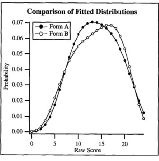
In the polynomial loglinear model shown in Table 3, λT_j is the forms effect, k is the number of items, and d represents the number of polynomial degrees (where d ranges from 1 to 10). In the full model, the first d moments of the estimated distribution are the same as the first d moments of the observed distributions. In other words, if d=2, then the mean and standard deviation of the expected frequencies will be the same as those for the observed frequencies on Form A. The same will be true on Form B. This is not true for the estimated distributions in the reduced model because the distributions for Form X and Form Y are constrained to be the same. All estimated frequencies will be estimated so that the distributions are the same on both forms of the examination. The purpose of this is to compare these two models and determine which is a better fit to the data.

chi-square values are estimated. Interpretation of the statistics is described next in the context of an example from Hanson’s study.

Application of the Hanson Method

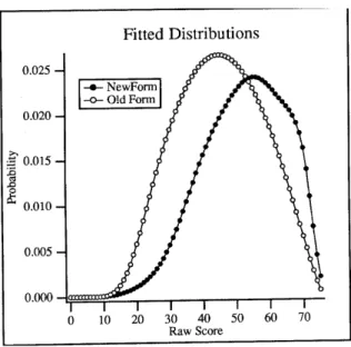
Hanson (1996) applied the methodology just described using two data sets. Figure 2 and Tables 4 and 5 summarize the data and results from one of those examples. The data for this example came from two-forms of a 24-item, ACT elementary algebra examination. Figure 2 presents the cumulative frequency distribution, and the first two lines of Table 4 present the descriptive statistics (labeled SDP1, Score Distribution Pair 1).

---Insert Figure 2 about here.--- ---Insert Table 4 about here.--- ---Insert Table 5 about here.---

Table 5 gives the results of Hanson’s (1996) method for detecting differences in score distributions using the polynomial loglinear model. The table provides the chi-square statistic associated with each polynomial degree (Degree), the degrees of freedom (df), a difference calculation (Difference) for both the full and reduced models, and a summary column (Test of Distribution Difference). The Difference column calculates the difference in the chi-square value between a particular polynomial degree and the previous one.

associated with the alternative hypothesis is the model that will be selected. The null hypothesis is rejected when a significant chi-squarevalue is reached. The alternative hypothesis (d=d*+1) is then chosen.

In the example, the chi-square values were compared using an alpha level of .001 (to adjust for nine comparisons) with two degrees of freedom (equal to number of chi-square values being compared to determine the fit of a single polynomial degree), which is a chi-squarevalue of 13.82 or larger. For the Full Model in Table 5, starting with 10 polynomial degrees and moving down, and looking at the Difference column, the first degree where the difference exceeds 13.82 is d=3 (Difference=131.78). The null hypothesis that d=3 (d*=3) is rejected, and the alternative hypothesis d=4 (d=d*+1) is accepted. The same process can be used to determine the desired Degree by looking at the Reduced Model. Only one model needs to be analyzed to select the degree.

Once the polynomial degree is selected, the last three columns (Test for Distribution Differences) are the actual comparison of the distributions. The polynomial degree selected in this example was 4 (d=3+1). At d=4 (under column df), the

χ

As mentioned earlier, the Hanson (1996) method has been recommended in the literature for determining whether to equate scores on two or more forms a test, in general, and specifically when there are only small samples of data available for equating. The Hanson method makes assumptions about the similarity of the sampled populations by comparing the score distributions between forms. When the results indicate that

distributions are the same, the samples from the two forms are considered to be drawn from the same population, and no equating is necessary. Alternatively, when the results indicate that the distributions are different, the samples are assumed to come from different

populations, and equating is necessary.

III. METHODOLOGY

This study was conducted using a Monte Carlo design. Data were simulated and Hanson’s (1996) method for determining differences in distributions applied using a SAS 9.1 program designed for this study. (The SAS code used is provided in the Appendix.) The two steps--simulating the data and applying the Hanson method--were combined into one program for the purpose of simulating and running each test multiple (n=1000) times.

Three pairs of distributions with varying standardized mean differences (SMDs) were compared. Figure 2 and 4 show plots and descriptive statistics for the original pair of distributions that were taken from Hanson’s (1996) study for testing differences in

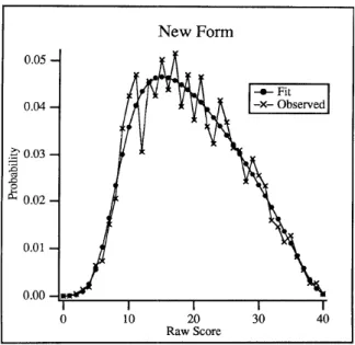
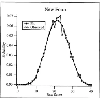
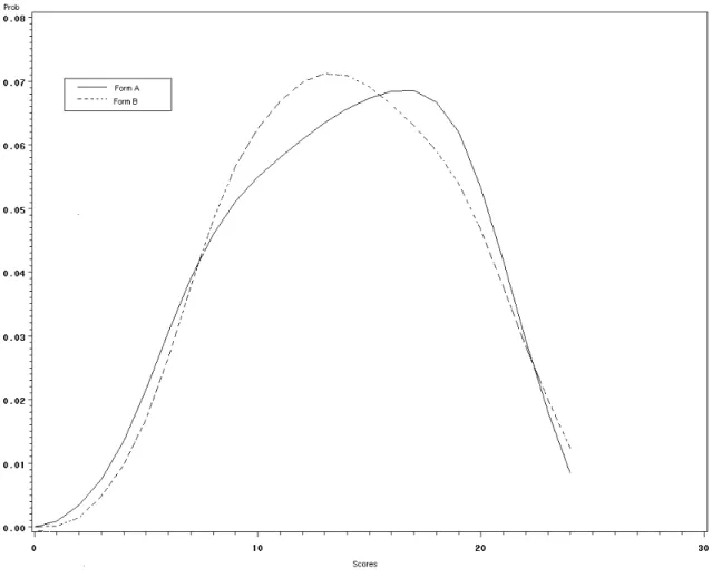
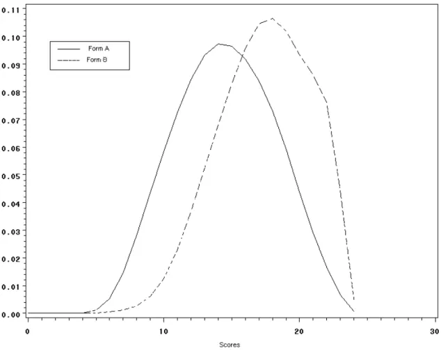
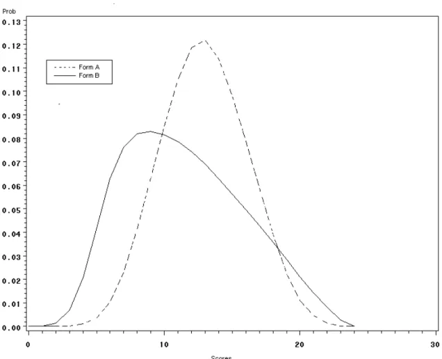
distributions. The second and third pairs were adapted from Hanson, Zang, and Colton (1994; Figures 3, 4, 5, Table 4). These distributions are loglinear-smoothed estimates of population scores based on six forms of four different ACT tests.

---Insert Figures 2-5 about here.---

Figure 2 shows two distributions from two forms (Form A and Form B) of an ACT elementary algebra assessment (Hanson, 1996). This pair of distributions will be referred to as Score Distribution Pair 1 (SDP1). Descriptive statistics for the original SDP1 are shown in 4. This is the same pair of distributions used in the example of Hanson’s method

discussed above. Recall that in this example, with n=3293, the null hypothesis that

The purpose of using this example for the current study was to be able to determine whether the null hypothesis could still be rejected when sample size (n) is reduced.

However, the means of the Form A and Form B distributions are extremely close (13.93 13.99, respectively). The SMDs between the two forms using an averaged standard deviation (4.92) is only .01, indicating the degree to which these two forms differ in difficulty is very small (Howell, 2002). In reality, it would be unlikely that two forms of a test could be constructed with this much precision. For this reason, two additional pairs of distributions were examined to determine how the Hanson (1996) method might perform for small sample sizes when there is a greater SMD. A summary of SMDs for all three pairs of distributions is provided in Table 6.

---Insert Table 6 about here.---

The distributions from the second pair of distributions (SDP2, shown in Figures 3 and 4), are a simulated pair of distributions resulting from a combination of one form from each of two 40-item tests covering different subject matter. The purpose of creating SDP2 was to test a pair of distributions that had a larger but moderate SMD compared to SDP1. The approximate SMD for this example is .31, using an averaged standard deviation of 6.71.

retesting. In this example, the scores on the first administration would be expected to be higher than those on the second administration.

The process for extracting data from these original distributions and applying it to the SAS program, which generates a data simulation and applies the Hanson (1996) method, is presented in graphical form in Figure 6. The figure shows that the graphical representation of the original distributions (SDP1) was used to find the probabilities for each raw score (SDP2) using Datathief (Tummus, 2006). Datathief is a program designed to generate data from graphical representations. The distributions derived from this process were first applied to a SAS program (see Appendix) that converted the probabilities seen in Step 2 to the file shown in Step 3. The data in Step 3 are (going from left to right): the item count, raw score, cumulative density functions of y1 and y2 (Forms A and B), and the cumulative distribution functions of y1 and y2.

---Insert Figure 6 about here.---

In Step 4, the SAS program used the information described in Step 3 to first simulate distributions, and then apply the Hanson (1996) method as described in the previous section and example. This process was completed for sample sizes of 3500, 3000, 2500, 2000, 1500, 1000, 500, 250, 200, 150, 100, 50, and 25. The procedure was applied to each sample size 1000 times for all three distributions. The results, as indicated in Figure 6, were provided as two outputs: power and test summary. These are described in the Results and Discussion sections that follow.

and 7) and SMD as indicated in Table 6 (.008 for the simulated distributions). However, the statistics for the second and third pairs vary from the original data, although the graphical presentations are similar in shape for SDP2 and SDP3 and identical for SDP1 (Figures 7, 8, and 9). The reason for this difference is that it was desirable to transform SDP2 and SDP3 to the same scale as SDP1. In the end, all three pairs of distributions are presented on a scale of 0-24. This transformation was done while converting the data in Step 2 of Figure 6 to Step 3. The converted values in the distributions were then used for the simulation and method application.

---Insert Table 7 about here.--- ---Insert Figure 7-9 about here.---

IV. RESULTS

A primary result of this study was an estimation of power for each sample size within each pair of distributions. The box labeled “Output 1” in Figure 6 presents an example. The power estimation in these results indicates the frequency with which the method rejected the null hypothesis that the two score distributions being compared were different. For example, if power is .995, then the Hanson method rejected the null

hypothesis that distributions were the same 99.5 percent of the time indicating a high level of power.

Full results of the simulation are provided in Table 8. A comparison of all three score distribution pairs for each sample size is presented. The SDP is designated across the top of the table along with the SMD for each pair of distributions. The first column (n) indicates the sample size. Within each of the sections for a particular SDP there are three columns. The first column lists the polynomial degree or range of degrees selected for the particular sample size. This is the range across the 1000 iterations. For example, for SDP1 and n=3500, the polynomial degree range is 6-10 indicating that the method did not always select the same polynomial degree, but selected a value between 6 and 10.

---Insert Table 8 about here.---

The second column for each SDP is the Power over 1000 Iterations. This value indicates the percentage of times that the method rejected the null hypothesis that the distributions were the same. In the example just described (SDP1 and n=3500) the power is .995, indicating that the method rejected the null hypothesis nearly 100% of the time.

polynomial degree of one. Even when the test finds a significant difference between

distributions in this case it is comparing two straight lines and, thus, the results are not valid. For most of the sample sizes, for all three SDPs where power was 1 (or close to 1) in the second column, the polynomial degree was two or more; thus, the power estimates are the same in both the second and third columns. For example, for SDP1 and n=3500 the Power over 1000 Iterations is .995 and the Power When Polynomial Degree of Model > 1 is .995. When the sample size decreases to 50, the power estimates increase when considering only the iterations that selected a degree over 1. In the same example with sample size of 50, only 19 of the 1000 iterations used a polynomial degree over 1, and 47% of those 19

iterations found a significant difference between the distributions of scores on the two forms, rejecting the null hypothesis. The method never selected polynomial degrees over 1 for sample sizes of 25 for any of the three SDPs, meaning that a sample size of 25 is not adequate for fitting a density function to the scores on the two forms. The point at which the method completely breaks down, in the sense that it cannot estimate the density function, appears to be somewhere between 50 and 100.

V. CONCLUSIONS AND DISCUSSION

This study was designed to consider situations where multiple forms of an

examination are used for a testing program with small sample sizes (i.e., small numbers of examinees) and the determination must be made regarding whether or not to equate the forms. In these situations, decisions must be made about how similar forms are in difficulty and whether statistical methods should be applied to make scores on two different forms equivalent. Such decisions may be informed by using statistical methods such as the Hanson (1996) method for determining whether significant differences exist between score

distributions on two forms. The present study investigated the sensitivity of Hanson’s (1996) method to detect distributional differences when sample sizes are small.

power drops from .624 to .322, meaning that for a sample size of 1000, the method detects a difference between score distributions approximately 62% of the time and then drops to 32% when sample size is 500. For sample sizes under 100, the method detected differences only about 1% of the time.

It is important to note that the results do support use of the Hanson (1996) method for moderate sample sizes. The Hanson method may not work well for very small sample sizes (n=100), but there is evidence to support the use of the method for moderate sample sizes, depending on how large the difference is between the distributions. This study

indicates that when a somewhat moderate or very large difference (.33 or .82) is present, the method is able to detect differences between distributions for sample sizes over 100. Even when differences are very small, the method works most of the time for sample sizes between 1500 and 3000. The real issue with the method is for very small testing programs with similar score distributions.

Overall, the results suggest that the answer to the research question for SDP1 is not a simple one. The Hanson (1996) method is clearly less powerful as sample size decreases but, in the case of SDP1, it does so more gradually than the decrease in power for SDP2 and SDP3 because the differences between the forms are small.

Assessing whether a given sample size is adequate to determine important

differences between forms is clearer when test forms yield distributions of scores that have larger SMDs. For SDP2, the method detected differences 100% of the time for samples sizes of 150 or more, and most of the time for sample sizes of 100-200. There was a sharp,

that when there are significant differences between the forms, the point at which the method begins to break down is clearer than with forms that are more similar.

In addition to the SMD, the number of possible scores on the forms is a factor in how powerful the Hanson (1996) method is for determining differences between

distributions. Recall the earlier discussion of assumptions for the chi-square goodness of fit test and the impact that small sample sizes have on the estimation of expected values in the frequency table and resulting estimated score distributions. In the example from Hanson’s study and in the present study a particular score distribution is estimated using a 2-way contingency table for scores 0-24 ( 2x25 table) There are two columns corresponding to the two forms and 25 rows corresponding to the number of possible scores. For each form, there are 25 cells, meaning that if the sample size is small (e.g., 25), it is likely that there will be multiple cells with frequencies of zero and many with very small frequencies, violating the minimum cell frequency requirements for using this statistical test. This has an impact on the power of the statistical test. This issue is exacerbated when number of

possible scores increase. For example, an examination with 75 items (76 possible scores) will require a larger sample size for estimation of the chi-square statistic.

Overall, the results of this study indicate that, as would be expected, the Hanson (1996) method for detecting differences between score distributions has reduced power when sample size are small. What constitutes a small sample size has been discussed

multiple forms of an examination. The results of the study indicate that the definition of a small sample size depends on the SMD between forms. Forms that differ only slightly (as in SDP1) require larger sample sizes to detect differences than forms that have larger SMDs (as in SDP2 and SDP3).

The answer also depends on the stakes of the particular testing program. A high stakes testing program where important consequences are tied to the results of the examination may require more certainty in the results of the method than a low stakes testing that has limited consequences. For example, for a high stakes exam using two forms that have very small differences as in the example of SDP1, may require that the method detect important differences as close to 100% of the time as possible, meaning a large

sample size (over 3000) would be required. On the other hand, in a low stakes program with the same SMD, a smaller sample may be acceptable because the outcome is not as critical.

Second, the polynomial loglinear model needs a certain amount of data to estimate the density function of scores on two forms. The Hanson (1996) method selects a

polynomial degree for the model that is greater than one to adequately fit the distributions. For all three distributions, the model fit the data to a first-degree polynomial most of the time when sample sizes were under 100.

When using the Hanson (1996) method with samples of data under 1000, it is important to carefully review the cumulative frequency distributions and descriptive statistics to assess how much the forms differ and whether they differ in some areas more than in others. In this study, the SMD was used to determine such differences. This index, however, does not indicated that equating may be more necessary in areas where the scores differ more drastically than in others. The Hanson method compares score distributions overall as opposed to individual score levels. In the example of SDP1, the scores were more similar in the tails, around values of 8 and 15, and varied more in between. In these areas, scores may not need to be equated, while in other areas of the score scale equating may be necessary depending on the purpose of the testing program.

In the discussion of equating presented in Section II of this thesis, much of the literature recommended equating only near the mean when using small samples of data. The results of this study give an example of why this may be the best advice for a testing

null hypothesis would be retained as would be the case if distributional differences, such as those in SDP1, were present. Thus, the decision about form equating appears to depend to a great extent on how the scores are distributed for each form and, ultimately, how well the forms were constructed and data are collected. It is very unlikely that the Hanson method will detect differences in score distributions for small testing programs if a test developer has been attentive to all aspects of the testing process; that is, the test developer has defined the content domain well, constructed a detailed test specifications document, selected qualified SMEs, thoroughly trained those SMEs for item writing, technical review and standard-setting, provided adequate psychometric, grammatical, and technical edits, administered a well-conducted field test with examinees representative of the appropriate population, applied an appropriate testing model and carefully selected items, carefully assembled test forms based on the test specifications and statistics, and ensured equal reliability of forms.

That decision would affect the validity of the resulting scores because, in this example, scores from the two forms would be interpreted as being equivalent when, in fact, they are not.

The problem of potentially non-equivalent scores being interpreted as equivalent naturally extends to classification decisions based on those scores. This would be especially problematic in high stakes testing situations where the certification or licensure of an individual in a critical role, such as a physician or pilot, is involved and the relative costs of false positive and false negative decisions must be considered (Cizek, 2006). For example, a certification examination exists for high-level medical technicians using specialized

diagnostic equipment that may have small testing populations, but that are high-risk due to the potential harm to patients of certifying those not truly competent in the area (i.e., a false positive classification). It is critical for scores on forms of this examination to be equivalent. The equivalency of forms will affect whether a qualified candidate receives a passing score and an unqualified candidate does not. In the case where a qualified candidate fails the exam (a false-negative classification), this individual is unfairly barred from practicing in the chosen profession. Thus, careful consideration is needed in determining what constitutes similar forms through the comparison of score distributions.