Linear models with a generalized AR(1) covariance structure for longitudinal and spatial data

(1)

LINEAR MODELS WITH A GENERALIZED AR(1)

COVARIANCE STRUCTURE FOR LONGITUDINAL AND

SPATIAL DATA

Sean L. Simpson

A dissertation submitted to the faculty of the University of North Carolina at Chapel Hill in partial fulfillment of the requirements for the degree of Doctor of Philosophy in the

Department of Biostatistics, School of Public Health.

Chapel Hill 2008

Approved by:

Advisor: Lloyd J. Edwards

Reader: Keith E. Muller

Reader: Pranab K. Sen

Reader: Paul W. Stewart

(2)

(3)

ABSTRACT

SEAN L. SIMPSON. Linear Models with a Generalized AR(1) Covariance Structure for Longitudinal and Spatial Data.

(Under the direction of Dr. Lloyd J. Edwards)

Cross-sectional and longitudinal imaging studies are moving increasingly to the

forefront of medical research due to their ability to characterize spatial and spatiotemporal

features of biological structures across the lifespan. With Gaussian data, such designs require

the general linear model for repeated measures data when standard multivariate techniques do

not apply. A key advantage of this model lies in the flexibility of modeling the covariance of

the outcome as well as the mean. Proper specification of the covariance model can be

essential for the accurate estimation of and inference about the means and covariates of

interest.

Many repeated measures settings have within-subject correlation decreasing

exponentially in time or space. Even though observed correlations often decay at a much

slower or much faster rate than the AR(1) structure dictates, it sees the most use among the

variety of correlation patterns available. A three-parameter generalization of the

continuous-time AR(1) structure, termed the generalized autoregressive (GAR) covariance structure,

accommodates much slower and much faster correlation decay patterns. Special cases of the

GAR model include the AR(1) and equal correlation (as in compound symmetry) models.

The flexibility achieved with three parameters makes the GAR structure especially attractive

for the High Dimension, Low Sample Size case so common in medical imaging and various

kinds of "-omics" data. Excellent analytic and numerical properties help make the GAR

model a valuable addition to the suite of parsimonious covariance structures for repeated

(4)

iv

The accuracy of inference about the parameters of the GAR model in a moderately large

sample context is assessed. The GAR covariance model is shown to be far more robust to

misspecification in controlling fixed effect test size than the AR(1) model. It is as robust to

misspecification as another comparable model, the damped exponential (DE), while

possessing better statistical and convergence properties.

The GAR model is extended to the multivariate repeated measures context via the

development of a Kronecker product GAR covariance structure. This structure allows

modeling data in which the correlation between measurements for a given subject is induced

by two factors (e.g., spatio-temporal data). A key advantage of the model lies in the ease of

interpretation in terms of the independent contribution of every repeated factor to the overall

within-subject covariance matrix. The proposed model allows for an imbalance in both

dimensions across subjects.

Analyses of cross-sectional and longitudinal imaging data as well as strictly longitudinal

data demonstrate the benefits of the proposed models. Simulation studies further illustrate

the advantages of the methods. The demonstrated appeal of the models make it important to

pursue a variety of unanswered questions, especially in the areas of small sample properties

(5)

To Lorenzo, Jr. and Adelaide, for past enablements and present encouragement; to Lorenzo, Sr. and Bessie, for modeling commitment; to Gail for exemplifying selflessness and perseverance; to Marsha and Dennis for unmitigated support; and to Eva with a future in the

(6)

vi

ACKNOWLEDGMENTS

I must first thank my family whose love, support, and guidance have made my successes

possible and my obstacles surmountable. I am eternally indebted to my parents for their

selfless devotion to nurturing my interests and abilities.

I am extremely fortunate to have had Lloyd Edwards as my dissertation advisor. His

wisdom and insight have been immeasurable in facilitating my growth as a researcher and

preparing me for an academic career in biostatistics. His genuine advice and concern as a

mentor throughout my graduate career is a rarity for which I am immensely grateful. I owe

much gratitude to Keith Muller who also served as an advisor and mentor during my time at

Chapel Hill. He has been instrumental in fostering my development as a collaborator and

methodologist. I must also thank the other members of my committee: Pranab Sen, Paul

Stewart, and Martin Styner. They have each been more than willing to provide guidance and

insight as necessary. I thank Dale Zimmerman from the Department of Statistics and

Actuarial Science at the University of Iowa for the observation that the model can be

reparameterized to give further insight into its properties. I am also thankful to Chirayath

Suchindran for giving me the opportunity to serve as a trainee on NICHHD Training Grant

(7)

List Of Tables

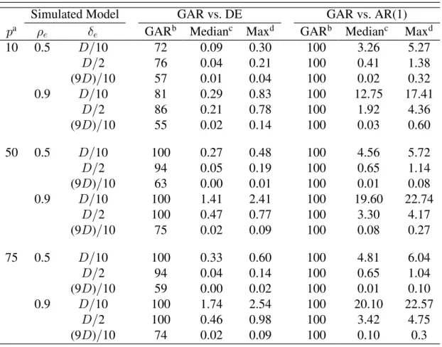
Table 2.1: Simulation results displaying the percent of realizations the GAR model

better fits the data according to the BIC, and the median and maximum

percent difference in BIC when this occurs. R œ "!! subjects and

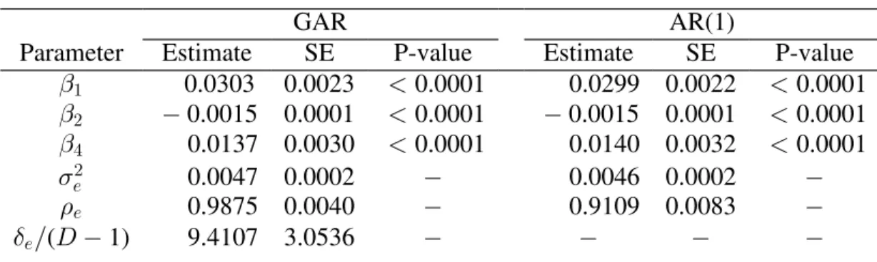
: œ : − "!ß &!ß (&3 e f observations each at unit distance intervals ... 38 Table 2.2: Final mean model estimates, standard errors, p-values, and covariance

parameter estimates for the neonate data... 39

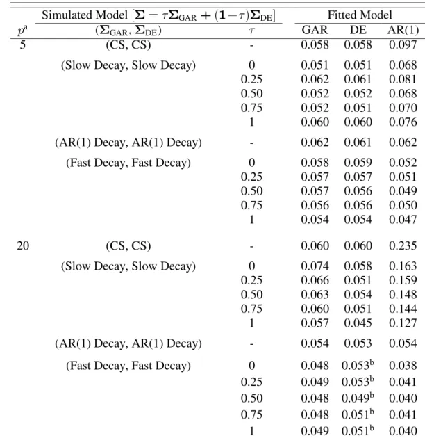
Table 3.1: Simulated fixed effect test size for the GAR, DE, and AR(1) models. Target αœ0.05, with R œ "!! subjects and : œ : − &ß #!3 e f

observations each at two-unit distance intervals...59

Table 3.2: Simulated covariance parameter test size for the GAR model. Target α œ0.05, with R œ "!! subjects and : œ : − &ß #!3 e f observations

each at two-unit distance intervals... 60

Table 3.3: Final mean model estimates, standard errors, p-values, and covariance

parameter estimates for the DASH data...61

Table 4.1: Simulations assessing the performance of the proposed estimation procedure for the Kronecker product GAR covariance model in a

moderately large-sample context. R œ "!! subjects and

> œ > œ "! ‚ = œ = œ "!3 3 observations each at two-unit

distance intervals...80

Table 4.2: BIC values for all combinations of factor specific covariance model fits

for the initial caudate data model...81

Table 4.3: Final covariance model estimates and standard errors for the caudate

(11)

List Of Figures

Figure 2.1: The lateral and ventral cortico-spinal tracts in the human nervous

system...40

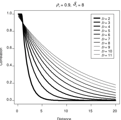
Figure 2.2: Plot of the various correlation patterns that can be obtained with the

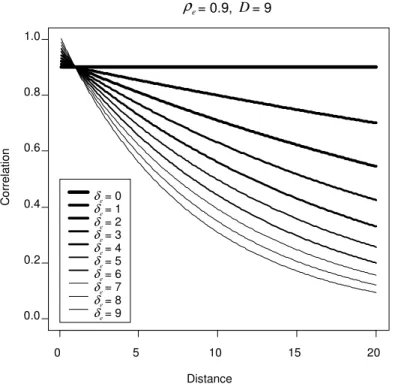
GAR model by varying the parameter while keeping and constant.$_/ 3_/ H

$_/ œ ) corresponds to an AR(1) decay rate, while $_/ œ ! corresponds to

compound symmetry...41

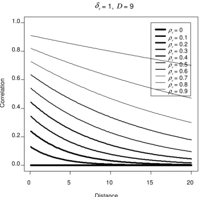
Figure 2.3: Plot of the various correlation patterns that can be obtained by varying the parameter while keeping and constant...423_/ $_/ H

Figure 2.4: Plot of the various correlation patterns that can be obtained by varying the constant while keeping and constant. H $_/ 3_/ H œ * corresponds to an

AR(1) decay rate... 43

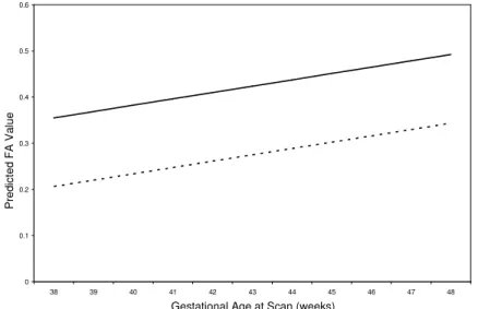
Figure 2.5: Predicted FA values for the neonates by location at the minimum (dashed line) and maximum (solid line) gestational ages at the time

of the scan...44

Figure 2.6: Predicted FA values for the neonates by the gestational age at the time

of the scan at the first (dashed line) and middle (solid line) locations...44

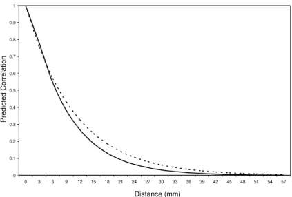
Figure 2.7: Predicted correlation curve for the best fitting GAR model (solid line) and AR(1) model (dashed line) as a function of the distance between

measurements for the neonate data... 45

Figure 3.1: Predicted correlation curve for the best fitting GAR model (solid line) and AR(1) model (dashed line) as a function of the distance between

measurements for the DASH data...62

Figure 4.1: Plot of correlation as a function of spatial and temporal distance when both factor specific matrices have a decay rate that is slower than that

of the AR(1) model... 83

Figure 4.2: Plot of correlation as a function of spatial and temporal distance when

both factor specific matrices have an AR(1) decay rate...84

Figure 4.3: Plot of correlation as a function of spatial and temporal distance when both factor specific matrices have a decay rate that is faster than that

of the AR(1) model... 85

(12)

xii

Figure 4.5: M-rep shape representation model of the caudate... 87

Figure 4.6: Predicted correlation as a function of the time between images for the

caudate data...88

Figure 4.7: Predicted correlation as a function of the distance between radius

locations for the caudate data...88

Figure 4.8: Predicted correlation as a function of the distance between radius

(13)

CHAPTER 1. INTRODUCTION AND LITERATURE

REVIEW

1.1 Introduction

Repeated measures studies are commonly utilized in biomedical research. Such

data allow examining how particular correlated outcomes vary over time or in space. In

longitudinal studies, measurements are taken on the same subjects at various points in

time. For instance, Rijcken et al. (1987) was interested in identifying risk factors for

pulmonary function loss. Therefore they recorded many baseline characteristics thought

to be possible risk factors, and attempted to measure FEV (forced expiratory volume in _" "

second) values every 3 years for 21 years to assess pulmonary function loss in terms of

the rate of decline.

In spatial studies, and more particularly in medical imaging studies, measurements

are taken on the same subjects at various points in space. The image of an organ in a

given subject is often characterized by the correlated (repeated) values resulting from the

mathematical parameterization of its shape. For example, Gerig et al. (2003) analyzed

changes of the hippocampal structure in schizophrenics as compared to matched controls

via MRI.

As technological advances continually reduce the financial and logistic obstacles

associated with the use of imaging equipment, imaging studies are becoming increasingly

important in medical research. This increasing importance was made evident by the

creation of the National Institute of Biomedical Imaging and Bioengineering at the

(14)

2

research units and centers have also been established by several universities in recent

years.

Current imaging research often utilizes a third hybrid type of repeated measures data,

namely spatio-temporal, that has both spatial and longitudinal components. The goal of

these studies is to analyze images taken over time. For instance, much of the current

Autism research involves examining the development of children's brains (via

neuroimaging) over time. Due to the frequency of the three types of repeated measures

data, the development of accurate analytic techniques for these studies is of immense

importance.

In repeated measures data, both the mean and the covariance are modeled. Though

modeling the mean is the primary focus of many studies, modeling the covariance

structure is one of the most fundamental and important concerns in the analysis of these

data. As noted by Louis (1988), there is a tradeoff between including additional

covariates in the mean model and increasing the complexity of the covariance structure.

In other words, the covariance structure may be able to account for the effects of

unmeasured covariates. Properly specifying the covariance model leads to more accurate

estimation of and inference about the covariates of interest. Having an accurately

specified covariance structure also allows for a better understanding of the biological

process under investigation.

While much work has been done on estimation, inference, and diagnostics of the

mean model (fixed effects), relatively little has been done in these areas for the

covariance model. Proper specification of the covariance model can be essential for the

accurate estimation of and inference about the means and covariates of interest. Muller et

al. (2007) showed that there can be severe test size inflation in fixed effect inference if the

covariance structure is badly misspecified. This heavy dependence of fixed-effects

(15)

amount of work on covariance models has not been commensurate with their level of

importance.

slower or much faster rate than the AR(1) structure dictates, it sees the most use among

the variety of correlation patterns available. In this dissertation I will propose a

three-parameter covariance model that is a generalization of the continuous-time AR(1)

structure which accommodates much slower and much faster correlation decay patterns.

1.2 Repeated Measures Model

Consider the following general linear model for repeated measures data:

C₃ œ\₃"/₃ (1.1) where C₃ is a _{: ‚ "}₃ vector of observations on the _:₃ ₃>2 subject _{3 œ "ß ÞÞÞß R}, _"is a _{; ‚ "}

vector of fixed and unknown population parameters, \₃ is a : ‚ ;₃ fixed and known

design matrix corresponding to the fixed effects, and is a /₃ : ‚ "₃ vector of random error

terms. We assume /₃ _{µ R Ð ß}_: ! _/3 _Ñ /₃ for _{3 Á 3}w. It follows

3 D Ð Ñ7/ and is independent of w

that C₃ _{µ R Ð}_: \₃ _ß _/3 _Ñ C₃ for _{3 Á 3}w. We also assume that

3 " D Ð Ñ7/ and is independent of w

D_/3Ð Ñ7_/ is a : ‚ :₃ ₃ positive-definite symmetric covariance matrix whose elements are

twice differentiable functions of a finite number of fixed, unknown parameters

7_/ œ Ö7_/_"ß ÞÞÞß7_/₅×, 7_/ −X, where is the set of all parameters for which X D_/3Ð Ñ7_/ is

positive-definite. Also, the parameters in 7_/are functionally independent of those in ."

The model may be abbreviated as C₃ µ R Ð:3 \₃" Dß /3Ñ.

The frequently used general linear mixed model, detailed by Laird and Ware (1982),

can be viewed as a special case of this model in which C3 œ\3"^ ,3 3/3 and

D 73Ð Ñ œ^3D,3Ð Ñ7, ^3wD/3Ð Ñ7/ , which may be abbreviated as D3 œ^3D,3^3w D/3.

We have that ^3 is a : ‚ 73 fixed and known design matrix corresponding to the random

(16)

4

effects, , which are mutually independent, and ,₃ D_/3 is the : ‚ :₃ ₃ positive-definite

symmetric covariance matrix of the random errors, , which are mutually independent./₃

It is assumed that ,₃ independent of .is /₃

1.3 Exponentially Decreasing Correlation 1.3.1 Introduction

The continuous-time first-order autoregressive covariance structure, often denoted as

AR(1), is the classic model applied to longitudinal and spatial data when the within

subject correlation is believed to decrease exponentially in time or space. For

longitudinal data this means that the correlation between measurements on a given

subject is assumed to decrease exponentially as the time between measurement occasions

increases. Analogously, this correlation is assumed to decrease exponentially as the

distance between measurement locations increases for spatial data. ForD_/3 œe5_/3à45f,

the AR(1) covariance structure is

5_/3à45 _{œ ÐC ß C Ñ œ}i ₃₄ ₃₅ 5_/# 3/.Ð> ß > Ñ34 35 4 Á 5

" 4 œ 5

 _, (1.2)

where iÐ † Ñ is the covariance operator,.Ð> ß > Ñ34 35 is the distance between measurement

times or locations, 5_/# is the variability of the measurements at each time or location, and

3/ is the correlation between observations separated by one unit of time or distance.

This two-parameter model was briefly discussed in Louis (1988) in an article surveying

methods for analyzing repeated measures data. It is a special case of the model presented

in Diggle (1988).

The AR(1) covariance model is particularly appealing when there are only a small

number of subjects with many observations per subject. It is also able to accommodate

incomplete unbalanced, (within subject), inconsistently-spaced, and/or irregularly-spaced

data which are all common issues in longitudinal studies. These problems may arise from

(17)

lengths of follow-up due to staggered entry or early withdrawal, and intentional unequal

spacing of measurements over time. Irregular-spacing may also be inherent in the

biological process being studied. For instance, a longitudinal study of pulmonary

function in children with cystic fibrosis may necessarily have this issue. Spatial data, and

more specifically medical imaging data, tend to be complete and balanced due to the tight

control typical of this area of research. However, irregular-spacing is again an issue with

these data that is easily handled with the AR(1) model. For this dissertation, it is assumed

that missing data is missing completely at random (MCAR).

Despite the utility of the AR(1) covariance model, there are situations in which it

may not be flexible enough to accurately model the correlation pattern induced by

repeatedly taking measurements over time or in space. For instance, as noted in Munoz et

al. (1992), longitudinal studies in epidemiologic settings tend to have within-subject

correlations that decay at a slower rate than that imposed by the AR(1) structure.

Conversely, there are also many situations in both longitudinal and imaging data in which

these correlations decay at faster rate. Therefore, developing a more flexible version ofa

the AR(1) model would be extremely beneficial to the scientific community.

1.3.2 AR(1) Generalizations

LaVange and Muller (1992) described a three-parameter generalization of the AR(1)

structure as a tool for power analysis in repeated measures studies, but did not discuss any

properties or consider estimation. They defined the model in order to be able to generate

a realistic suite of possible repeated measures covariance models in terms of only three

parameters. The appeal of the model led the author of NQuery power software to®

embed the model in the software as a study planning tool.

Munoz et al. (1992) presented a three-parameter generalization of the AR(1)

structure, namely the damped exponential (DE) structure, which allows for an attenuation

(18)

6

(1990) described the same model in an unpublished dissertation. ForD_/3 œ e5_/3à45f, the

damped exponential (DE) covariance structure is

5/3à45 i 34 35 5/# 3/

34 35

œ ÐC ß C Ñ œ .Ð> ß > Ñ 4 Á 5

" 4 œ 5

 c d

//

, (1.3)

times or locations, 5_/# is the variability of the measurements at each time or location, is3

/

the correlation between observations separated by one unit of time or distance and isß /_/

the decay speed. They assume ! Ÿ3_/ ' " and ! Ÿ/_/.

Implicit in this model formulation is the presence of both a stationary variance and

correlation structure. The AR(1) covariance model is a special case of this model for

which // œ ". For values of // ( ", the correlation between measurements on a given subject decreases in time or space at a faster rate than for // œ ". As // Ä ∞, this model

approaches the moving average model of order 1, MA(1). For values of such that//

! '// ' ", the correlation between measurements on a given subject decreases in time

or space at a slower rate than for // œ ". When // œ !, this model reduces to the well known compound symmetric covariance model for which the correlation between

measurements on a given subject is fixed at no matter how far apart in time or space3/

the measurements were taken. Though values of // ' ! yield valid autocorrelation

functions for which the correlation between measurements on a given subject would

increase with increasing time or distance between measurements, this is rare in

biostatistical applications. Therefore the parameter space was restricted for reasons of

practicality.

Nunez-Anton and Woodworth (1994) also proposed a three-parameter covariance

model to deal with incomplete unbalanced, , and irregularly-spaced longitudinal data. For

(19)

5 i 5

3

-3

-/3à45 34 35 /#

/ 34 35 /

œ ÐC ß C Ñ œ

Ð> + > Ñ

4 Á 5ß Á !

691Ð> Î> Ñ

4 Á 5ß œ !

" 4 œ 5

Ú Ý Ý Û Ý Ý Ü

-/ -/

,

(1.4)

where iÐ † Ñ is the covariance operator,>34is the time or location of the 4>2 measurement

for subject 3, 5_/# is the variability of the measurements at each time or location, is the3 /

correlation between observations separated by one unit of time or distance when

-_/ œ "ßand -_/is the power transformation of time parameter. They assume ! Ÿ 3_/ ' ". This model differs from DE model in that it involves power transformations of time

rather than of time intervals. The AR(1) covariance model is a special case of this model

for which -_/ œ ". The models appeal lies in the fact that the power transformation can

produce nonstationary correlation structures for the within-subject errors, with stationary

correlation structures as a special case. In other words, the model can accommodate data

where the correlation between measurements for a given subject does not just depend on

the differences in time or location between two measurements, but also on the absolute

time or location of each individual measurement. However, the model lacks the

flexibility of the DE model when a stationary structure is assumed.

1.4 Maximum Likelihood Estimation 1.4.1 Overview

The goal of estimation is to estimate the parameters that characterize a given model

based on the available data. The basic approach of maximum likelihood (ML) estimation

is to find the parameter values that maximize the probability, or "likelihood", that the

observations would end up being equal to the observed data. In other words, find the

parameter values that are best supported by the observed data. An ML estimate, , of as)

vector of parameters, , maximizes the likelihood function of the parameters given the)

data. That is, if the likelihood function is denoted PÐ à ÑC ) , then the maximum value of

(20)

8

Under model 1.1, the set of measurements on a given individual are assumed to

follow a multivariate normal distribution with )œ Ö ß" 7/×, thus the likelihood function

of the parameters is given by

PÐ à ßC₃ " 7_/Ñ œ Ð# Ñ1 +8 Î#3 lD 7₃Ð Ñl_/ +"Î#_expÖ + ÐC₃+\₃" D 7Ñw ₃Ð Ñ Ð_/ +" C₃+\₃"ÑÎ#×_.

Since the measurements from different subjects are assumed to be mutually independent,

the joint likelihood function of all the measurements is the product of the R individual

likelihood functions. That is,

PÐ à ß Ñ œ PÐ à ß Ñ

œ Ð# Ñ l Ð Ñl Ö + Ð + Ñ Ð Ñ Ð + ÑÎ#×Þ

C C

C \ C \

" 7 " 7

D 7 " D 7 "

/ 3 /

3œ" R

+8 Î# +"Î# w +"

3 / 3 3 3 / 3 3

$

$ 1 3 _exp

The log-likelihood function, which is commonly used to derive the estimators, is thus

ln

ln ln

P œ 6Ð à ß Ñ

œ + 8 Ð# Ñ + " l Ð Ñl + " Ð + Ñ Ð Ñ Ð + ÑÞ

# # #

C

C \ C \

" 7

D 7 " D 7 "

/

3œ" 3œ" 3œ"

R R R

3

3 / 3 3 w 3 / +" 3 3

1

(1.5)

The MLE of is then"

"s œ_ Ds _ Ds

3œ" 3œ"

R R

3w 3 3w 3

+" +"

3 3

+"

\ \ \ C,

where Ds3 is the covariance matrix for with the MLE of , C3 7 7/ s/, inserted. Since it is generally not possible to express s7/in a closed form, the solution for given above is"s

not a closed form expression either, and thus their values must be found via numerical

algorithms.

1.4.2 Iterative Algorithms

Since the likelihood equations cannot usually be solved analytically for the general

(21)

employed. Many algorithms for this purpose have been proposed; however, the three

most commonly used are the Newton-Raphson, Fisher scoring, and EM algorithm. These

iterative techniques will be discussed in this section.

1.4.2.1 Newton-Raphson and Fisher Scoring Algorithms

Both the Newton-Raphson and Fisher scoring (also referred to as the method of

scoring) algorithms are based on the first and second-order partial derivatives of the

log-likelihood function. As detailed in Jennrich and Schluchter (1986) the Newton-Raphson

algorithm is an iterative procedure that computes new parameter values from current

values, with the (r1) iterate under model 1.1 with st ₎œ Ö ß_{" 7} × being:

/

)Ð<"Ñ œ)Ð<Ñ+L₎₎+"=) (1.6) where

L)) œ ` 6Î` ` ` 6Î` `

` 6Î` ` ` 6Î` `

” # # /•

# #

/ / /

" " " 7 7 " 7 7

=) œ `6Î`

`6Î` ” ₇"_/•

which are referred to as the Hessian matrix (or observed information matrix) and score

vector respectively. The Fisher scoring algorithm is identical to that of the

Newton-Raphson method except that the Hessian matrix is replaced by its expectation. This

matrix of expectations is commonly referred to as the expected information matrix.

As noted in Murray (1990) the Fisher scoring method may outperform the

Newton-Raphson procedure when the expected information matrix has a block diagonal structure.

Jennrich and Schluchter (1986) mentioned that the Fisher scoring method is also

preferred when the second derivatives of D₃ are nonzero since the Newton-Raphson

algorithm may require substantially more computation. However, the Newton-Raphson

(22)

10

may not always be computationally feasible. For both methods, constrained optimization

must normally be employed since the procedures may converge to maxima outside the

boundaries that ensure the positive-definiteness of D₃.

1.4.2.2 EM Algorithm

The EM algorithm, described by Dempster et al. (1977) is a two-step procedure

consisting of an expectation step (the E step) and a maximization step (the M step). The

conditional expectation of the log-likelihood given the observed data is taken in the E

step in order to estimate sufficient statistics for the complete data. The M step then

maximizes this conditional expectation in order to produce maximum likelihood

estimates of the parameters based on the sufficient statistics derived in the E step. The

method then iterates between the two steps until the estimates converge.

As noted by Wu (1983) the computation involved in the EM algorithm is often

relatively easy due to the nice form of the complete-data likelihood function. As a result,

the algorithm often uses less computation time per iteration than either the

Newton-Raphson or Fisher scoring method. The EM procedure also tends to use less computer

storage space than the other two methods. However, as mentioned by Murray (1990), the

EM algorithm does not directly produce covariance estimates for the estimators. It may

also require many more iterations to converge than the other two methods in many

practical situations. Jennrich and Schluchter (1986) proposed a hybrid algorithm, termed

the EM scoring algorithm, combining elements of the EM and Fisher scoring algorithms.

However, this method is only advantageous when D3 is a function of a large number of

parameters (e.g. large, unstructured D3). Lindstrom and Bates (1988) concluded that a

well-implemented Newton-Raphson algorithm is generally preferable to the EM

(23)

1.4.3 Finite Difference Approximations

All three commonly used iterative algorithms require derivative calculations. The

Newton-Raphson and Fisher scoring methods utilize first and second-order partial

derivatives of the log-likelihood function, while the EM method employs the first partial

derivatives of the conditional expectation of the log-likelihood given the observed data.

The finite difference approximations of these derivatives are useful when exact analytical

derivatives are unwieldy or difficult to obtain. The forward and central difference

derivative approximations are the two main types of these approximations.

As noted by SAS documentation (SAS Institute, 1999), the forward difference

derivative approximations are often not as precise as the central difference derivative

approximations, though they do use less computer time. For first-order derivatives the

forward difference derivative approximations require additional objective function8

calls, where is the number of parameters. These approximations are computed as8

1 œ `0 ¸ 0 Ð 2 Ñ + 0 Ð Ñ

` 2

3

3 3

3 3 )

) / )

,

where is the /3 3>2 unit vector and is the 23 3>2 step size, 3 œ "ß ÞÞÞß 8. Dennis and

Schnabel (1983) detailed the forward difference approximation formulas for the Hessian

matrix. An additional 8 8 Î## function calls are required for second-order derivative

approximations based on only the objective function, which are calculated as

` 0

` ` ¸ 2 2

0 Ð 2 2 Ñ + 0 Ð 2 Ñ + 0 Ð 2 Ñ 0 Ð Ñ

#

3 4 3 4

3 3 4 4 3 3 4 4

) )

) / / ) / ) / )

.

Second-order derivative approximations based on the gradient vector, which only require

8 additional gradient calls, are computed as

` 0

` ` ¸ #2 #2

1 Ð 2 Ñ + 1 Ð Ñ 1 Ð 2 Ñ + 1 Ð Ñ

#

3 4 4 3

3 4 4 3 4 3 3 4

) )

) / ) ) / )

(24)

12

The more precise, but more computationally intensive central difference derivative

approximation formulas are presented below. For first-order derivatives the

approximations, which take an additional #8objective function calls, are computed as

1 œ `0 ¸ 0 Ð 2 Ñ + 0 Ð + 2 Ñ

` #2

3

3 3

3 3 3 3

)

) / ) /

.

Abramowitz and Stegun (1972) detailed the central difference approximation formulas

for the Hessian matrix. An additional #8 #8# function calls are required for

second-order derivative approximations based on only the objective function, which are

calculated as

` 0 + 0 Ð #2 Ñ "'0 Ð 2 Ñ + $!0 Ð Ñ "'0 Ð + 2 Ñ + 0 Ð + #2 Ñ

` ¸ "#2

#

3 3

# #

3 3 3 3 3 3 3 3

)

) / ) / ) ) / ) /

,

` 0

` ` ¸ %2 2

0 Ð 2 2 Ñ+0 Ð 2 +2 Ñ+0 Ð +2 2 Ñ0 Ð +2 +2 Ñ

#

3 4 3 4

3 3 4 4 3 3 4 4 3 3 4 4 3 3 4 4

) )

) / / ) / / ) / / ) / /

.

Second-order derivative approximations based on the gradient vector, requiring #8

additional gradient calls, are computed as

` 0

` ` ¸ %2 %2

1 Ð 2 Ñ + 1 Ð + 2 Ñ 1 Ð 2 Ñ + 1 Ð + 2 Ñ

#

3 4 4 3

3 4 4 3 4 4 4 3 3 4 3 3

) )

) / ) / ) / ) /

.

The step sizes, , for the forward difference approximations of the first-order23

derivatives based on objective function calls and the second-order derivatives based on

gradient calls are defined as

2 œ3 È# (Ð" l lÑ)3 .

For the forward difference approximations of second-order derivatives based only on

objective function calls and for all central difference formulas the step sizes are

2 œ3 È$ (Ð" l lÑ)3 .

(25)

1.5 Kronecker Product Covariance Structures 1.5.1 Overview

Multivariate repeated measures studies are characterized by data that have more than

one set of correlated outcomes or repeated factors. Spatio-temporal data fall into this

more general category since the outcome variables are repeated in both space and time.

When analyzing multivariate repeated measures data, it is often advantageous to model

the covariance separately for each repeated factor. This method of modeling the

covariance utilizes the Kronecker product to combine the factor specific covariance

structures into an overall covariance model.

Kronecker product covariance structures, also known as separable covariance

models, were first introduced by Galecki (1994). A covariance matrix is separable if and

only if it can be written as DœZ ŒW. He noted that one of the model's main

advantages is the ease of interpretation in terms of the independent contribution of every

repeated factor to the overall within-subject covariance matrix. The model also allows

for covariance matrices with nested parameter spaces and factor specific within-subject

variance heterogeneity. Galecki (1994), along with Mitchell et al. (2006) and Naik and

Rao (2001), detailed the numerous computational advantages of the Kronecker product

covariance structure. Since all calculations can be performed on the smaller dimensional

factor specific models, the computation of the partial derivatives, inverse, and the

Cholesky decomposition of the overall covariance matrix is relatively easier.

Despite the many benefits of separable covariance models, they have limitations. As

mentioned by Cressie and Huang (1999), the interaction among the various factors cannot

be modeled when utilizing a Kronecker product structure. Galecki (1994), Huizenga et

al. (2002), and Mitchell et al. (2006) all noted that a lack of identifiability can result with

this model. This indeterminacy stems from the fact that if Dœ>ŒH is the overall

(26)

14

+ Œ Ð"Î+Ñ> Hœ>ŒH. However, this nonidentifiability can be fixed by rescaling one of the factor specific covariance matrices so that one of its diagonal nonzero elements is

equal to . With homogeneous variances, this rescaled matrix is a correlation matrix."

Several tests of separability have been developed to determine whether a separable

or nonseparable covariance model is most appropriate. Shitan and Brockwell (1995)

constructed an asymptotic chi-square test for separability. A likelihood ratio test for

separability was derived by Mitchell et al. (2006) and Lu and Zimmerman (2005).

Fuentes (2006) developed a test for separability of a spatio-temporal process utilizing

spectral methods. All of these tests were developed for complete and balanced data.

Given that in many situations multivariate repeated measures data are unbalanced in at

least one of the factors, more general tests for separability need to be developed.

There is also a lack of literature on the estimation of separable covariance models

when there is an imbalance in at least one dimension. Only Naik (2001) examined the

case in which data may be unbalanced in one of the factors, namely D3 œZ ŒW3. This

situation arises often in spatio-temporal studies since the data tend to be balanced in

space, but not in time. However, there are multivariate repeated measures studies in

which the data are unbalanced in both dimensions, namely D3 œZ3ŒW3. This case has

yet to be examined in the literature.

With the assumptions of covariance model separability and homoscedasticity, an

equal variance Kronecker product structure has great appeal. In this case the overall

within-subject covariance matrix is defined as D₃ _œ₅#> _ŒH₃. This formulation has

3

several advantages. The reduction in the number of parameters leads to computational

(27)

1.5.2 Multivariate Repeated Measures Model with Kronecker Product Covariance

Consider the following general linear model with structured covariance for repeated

measures data:

C3 œ\3"/3 (1.7)

where C₃ is a _> vector of _> observations on the >2 subject , is a

3 3= ‚ " 3 3= 3 3 œ "ß ÞÞÞß R "

; ‚ " vector of fixed and unknown population parameters, \₃ is a >3 3= ‚ ; fixed and known design matrix corresponding to the fixed effects, , and is a " /₃ >3 3= ‚ " vector of

random error terms. We assume /₃ _{µ R} ₌_{Ð ß}! _/3_Ð _/#_ß _/_{Ñ œ} _/#_Ò _Ð _/ _{Ñ Œ} _/3_Ð _/ _ÑÓÑ

>3 3 D 5 7 5 >/3 7 # H 7 =

and is independent of /₃_w for _{3 Á 3}w. It follows that

C₃ _{µ R}_> _Ð\₃ _ß _Ð _{Ñ œ} #_Ò _/3_Ð _{Ñ Œ} _Ð _ÑÓÑ C₃

3 3= /3 / / / / /3 / w

#

" D 5 ß7 5 > 7 # H 7 = and is independent of for

3 Á 3w > >

/3 3 3

. We assume that > Ð7/#Ñ is a ‚ positive-definite symmetric correlation

matrix whose elements are twice differentiable functions of a finite number of fixed,

unknown parameters 7_/_# œ Ö7_/_#_"ß ÞÞÞß7_/_#₅×, 7_/_#%X#, where X# is the set of all

parameters for which >_/3Ð7/#Ñ is positive-definite. We also assume that H/3Ð7/=Ñ is a

= ‚ =3 3 positive-definite symmetric correlation matrix whose elements are twice

differentiable functions of a finite number of fixed, unknown parameters

7_/₌ œ Ö7_/₌_"ß ÞÞÞß7_/₌₅×, 7_/₌%X=, where X= is the set of all parameters for which H_/3Ð7_/₌Ñ

is positive-definite. This implies that D_/3_Ð₅_/#_ß7_/_Ñ is an _> _{= ‚ =}_> positive-definite

3 3 3 3

symmetric covariance matrix whose elements are twice differentiable functions of a finite

number of fixed, unknown parameters 5_/# and , , where is the set

/ / / /

7 œÖ7 #à7 =× 7 %X X

of all parameters for which D_/3_Ð₅_/#_ß7_/_Ñ is positive-definite._The parameters in e₅_/#_ß7_/f

are assumed to be functionally independent of those in . The model may be abbreviated"

as C₃ _{µ R}_> _Ð\₃ _ß _œ #_Ò _/3_Œ _ÓÑ

(28)

16

1.6 Inference

Likelihood-based statistics are generally used for inference concerning the

covariance parameters in the general linear model for repeated measures data. The three

most common methods of this type being the Likelihood Ratio, Wald, and Score tests.

Chi and Reinsel (1989) utilized the Score test for making inferences about the correlation

parameter in the random errors of a model for longitudinal data with random effects and

an AR(1) random error structure. However, this test was only used for reasons of

simplicity in the context of testing for the presence of autocorrelation versus

independence in the random errors of a mixed model. Jones and Boadi-Boateng (1991)

employed both the Wald and Likelihood Ratio tests to make inferences about the

nonlinear covariance parameters of irregularly-spaced longitudinal data with an AR(1)

random error structure. They noted that the Likelihood Ratio method is the most

effective way of testing the significance of the nonlinear parameters. The Wald test does

not always perform as well since the covariance matrix of these parameters is estimated

using a numerical approximation of the information matrix. It was also noted in Verbeke

and Molenberghs (2000) that the Wald test is valid for large samples, but that it can be

unreliable for small samples and for parameters known to have skewed or bounded

distributions, as is the case for most covariance parameters. They too recommend use of

the Likelihood Ratio Test for covariance parameter inference. Yokoyama (1997)

proposed a modified Likelihood Ratio test for performing inference on the covariance

parameters. However, this was only employed in lieu of the normal Likelihood Ratio

Test because its computation was too complex in their context of having a multivariate

random-effects covariance structure in a multivariate growth curve model with differing

numbers of random effects.

Neyman and Pearson (1928) first proposed the Likelihood Ratio Test. We generally

(29)

L À! )> œ)>ß!

(1.8)

L À" )> Á)>ß!

where )_>ß! is a vector of constants and )_œ _{Ð ß}) )_>w ₈w w_Ñ. The vector contains the test)_>

parameters, the parameters of interest on which inference is to be performed. The )₈

vector contains the nuisance parameters which must be estimated in order to utilize the

Likelihood Ratio Method. Denoting the parameter spaces under L! (the null hypothesis)

and L" (the alternative hypothesis) as and , respectively, the test statistic for the# > Likelihood Ratio Method is

A %#

%>

œ œ

PÐ à Ñ PÐ à Ñ

PÐ às Ñ

max

) )

C C

#

>

(1.9)

where )s# and )s> are the estimates of the parameters of the model under the null and alternative hypotheses respectively. Often this statistic is written as

+ #lnAœ #Ò6Ð àC s)>Ñ + 6Ð àC s)#ÑÓ (1.10)

which, under most conditions, is asymptotically distributed as a ;# random variable The

< Þ

degrees of freedom, , is equal to the number of linearly independent restrictions imposed<

on the parameter space by the null hypothesis. As noted by Self and Liang (1987), if the

model resides on the boundary of the covariance parameter space under the null

hypothesis, the asymptotic distribution of the test statistic in equation 1.10 becomes a

mixture of ;# distributions.

1.7 Summary

Repeated measures designs with incomplete unbalanced, (within subject),

(30)

spatio-18

temporal data, with medical imaging data being at the forefront of spatial and

spatio-temporal research. With Gaussian data, such designs require the general linear model for

repeated measures data when standard multivariate techniques do not apply.

slower or much faster rate than the AR(1) structure dictates, it sees the most use among

the variety of correlation patterns available. Munoz et al. (1992) presented a

parsimonious three-parameter generalization of the AR(1) structure, namely the DE

structure, which allows for an attenuation or acceleration of the exponential decay rate

imposed by the AR(1) structure. Nunez-Anton and Woodworth (1994) also proposed a

three-parameter covariance model for repeated measures data that allows for

nonstationary correlation structures for the within-subject errors; however, it lacks the

flexibility of the DE model when the data are assumed to have a stationary structure,

which is often the case.

In this dissertation I will propose a three-parameter covariance model that is a

generalization of the continuous-time AR(1) structure. I will show that this new model,

termed the generalized autoregressive (GAR) covariance structure, is more appropriate

for many types of data than the AR(1) model. I also will make evident that the GAR

model is more flexible than the DE covariance structure. However, merely showing that

the two models are different is sufficient for the relevance of the GAR since the aim is

not to replace other models, but to add to the suite of parsimonious covariance structures

for repeated measures data. The GAR model is proposed in Chapter 2 along with the

derivations of the estimates of its parameters and the variances of those estimates for

confidence interval construction. Chapter 3 examines inference about the parameters of

(31)

setting in which a Kronecker product covariance model is employed. Chapter 5

(32)

CHAPTER 2. ESTIMATION IN LINEAR MODELS WITH A

GENERALIZED AR(1) COVARIANCE STRUCTURE

2.1 Introduction 2.1.1 Motivation

Repeated measures designs with incomplete unbalanced, (within subject),

inconsistently-spaced, and irregularly-spaced data are quite prevalent in biomedical research. These studies are often employed to examine longitudinal, spatial, or

temporal data, with medical imaging data being at the forefront of spatial and

spatio-temporal research. Accurately modeling the covariance structure of these types of data

can be of immense importance for proper analyses to be conducted. Louis (1988) noted

that there is a tradeoff between including additional covariates and increasing the

complexity of the covariance structure. The covariance structure may be able to account

for the effects of unmeasured fixed effect covariates. Proper specification of the

covariance model can be essential for the accurate estimation of and inference about the

means and covariates of interest. Muller et al. (2007) showed that there can be severe test

size inflation in fixed effect inference if the covariance structure is badly misspecified.

exponentially in time or space. The continuous-time first-order autoregressive covariance

structure, denoted AR(1), sees the most utilization among the variety of correlation

patterns available in this context. This two-parameter model was briefly examined by

Louis (1988) and is a special case of the model described by Diggle (1988). The AR(1)

covariance model is very widely used; however, there are situations in which it may not

(33)

taking measurements over time or in space. In both longitudinal and imaging studies the

within-subject correlations often decay at a slower or faster rate than that imposed by the

AR(1) structure. Thus, a more flexible version of the AR(1) model is needed. Due to the

desire to maintain parsimony, only three-parameter generalizations are considered.

The emphasis on covariance models with a modest number of parameters reflects the

desire to accommodate a variety of kinds of real data. Missing and mis-timed data

typically occur in longitudinal research, while High Dimension, Low Sample Size

(HDLSS) data occur with imaging, metabolomics, genomics, etc. The inevitable and ever

more common scientific use of longitudinal studies of imaging only increases the

pressure to expand the suite of flexible and credible covariance models based on a small

number of parameters.

A three-parameter generalization of the continuous-time AR(1) structure, termed the

generalized autoregressive (GAR) covariance structure, which is more appropriate for

many types of data than comparable models is proposed in this chapter. Special cases of

the GAR model include the AR(1) and equal correlation (as in compound symmetry)

models. The flexibility achieved with three parameters makes the GAR structure

especially attractive for the High Dimension, Low Sample Size case so common in

medical imaging and various kinds of "-omics" data. Excellent analytic and numerical

properties help make the GAR model a valuable addition to the suite of parsimonious

covariance structures for repeated measures data.

Section 2.2 provides a formal definition of the GAR model as well as parameter

estimators and their variances. Graphical comparisons across parameter values illustrate

the flexibility of the GAR model. Simulation studies in section 2.3 help compare the

AR(1), DE, and GAR models. I discuss the analysis of an example dataset in section 2.4

(34)

22

2.1.2 Literature Review

LaVange and Muller (1992) described a three-parameter generalization of the AR(1)

structure as a tool for power analysis in repeated measures studies, but did not discuss any

properties or consider estimation. They defined the model in order to be able to generate

a realistic suite of possible repeated measures covariance models in terms of only three

parameters. The appeal of the model led the author of NQuery power software to®

embed the model in the software as a study planning tool. Munoz et al. (1992) presented

a three-parameter generalization of the AR(1) structure, namely the damped exponential

(DE) structure, which allows for an attenuation or acceleration of the exponential decay

rate imposed by the AR(1) structure. Murray (1990) described the same model in an

unpublished dissertation. As noted by Grady and Helms (1995), the DE model has issues

with convergence due to its parameterization. Nunez-Anton and Woodworth (1994)

proposed a three-parameter covariance model that allows for nonstationary correlation for

the within-subject errors. The model lacks the flexibility of the DE model when a

stationary structure is assumed.

Proper estimation of fixed effect and covariance parameters in a repeated measures

model requires iterative numerical algorithms. Jennrich and Schluchter (1986) detailed

the Newton-Raphson and Fisher scoring algorithms for maximum likelihood (ML)

estimation of model parameters. Dempster et al. (1977) first proposed the EM algorithm

for parameter estimation. The Newton-Raphson method is more widely applicable than

the Fisher scoring method due to the computational infeasibility of calculating the

expected information matrix in certain contexts. As noted by Lindstrom and Bates

(1988), the method is also generally preferable to the EM procedure.

The benefits of profiling out 5#and optimizing the resulting profile log-likelihood to

derive model parameter estimates via the Newton-Raphson algorithm was discussed by

(35)

fewer iterations, will have simpler derivatives, and the convergence will be more

consistent. There are also certain situations in which the Newton-Raphson algorithm may

fail to converge when optimizing the original log-likelihood but converge with ease

utilizing the profile log-likelihood.

2.2 GAR Covariance Model 2.2.1 Notation

Consider the following general linear model for repeated measures data with the

GAR covariance structure:

C3 œ\3"/3 (2.1)

where C₃ is a _{: ‚ "}₃ vector of observations on the _:₃ ₃>2 subject _{3 œ "ß ÞÞÞß R}, _"is a _{; ‚ "}

vector of fixed and unknown population parameters, \₃ is a : ‚ ;₃ fixed and known

design matrix corresponding to the fixed effects, and is a /₃ : ‚ "₃ vector of random error

terms. We assume /₃ _{µ R Ð ß}_: ! _/3_Ñ /₃ for _{3 Á 3}w. It follows that

3 D and is independent of w

C₃ _{µ R Ð}_: \₃ _ß _/3_Ñ C₃ _{3 Á 3}w

3 " D and is independent of w for .

ForD_/3 œ e5_/3à45f, the generalized autoregressive(GAR) covariance structure is

5_/3à45 _{œ ÐC ß C Ñ œ}i ₃₄ ₃₅ 5_/# 3/" Ð.Ð> ß > Ñ + "Ñ ÎÐH + Ñ34 35 $/ 4 Á 5

" 4 œ 5

 c 1 d _, (2.2)

times or locations, is a computational flexibility H constant that can be specified and by

default it is set to the maximum number of distance units, 5_/# is the variability of the

measurements at each time or location, is the correlation between observations3_/

separated by one unit of time or distance and is the decay speed. We assumeß $_/

! Ÿ3_/ ' "ß ! Ÿ $_/ßand H ( ".

Implicit in this model formulation is the presence of both a stationary variance and

(36)

24

which $_/ œ H + ". For values of $_/ ( H + ", the correlation between measurements on

a given subject decreases in time or space at a faster rate than for $_/ œ H + ". As

$_/ Ä ∞, this model approaches the moving average model of order 1, MA(1). For

values of such that $_/ ! '$_/ ' H + ", the correlation between measurements on a given

subject decreases in time or space at a slower rate than for $_/ œ H + ". When $_/ œ !,

this model reduces to the well known compound symmetric covariance model for which

the correlation between measurements on a given subject is fixed at no matter how far3_/

apart in time or space the measurements were taken. Though values of $_/' ! yield valid

autocorrelation functions for which the correlation between measurements on a given

subject would increase with increasing time or distance between measurements, this is

rare in biostatistical applications. Therefore the parameter space is restricted for reasons

of practicality.

2.2.2 Plots

Graphical depictions of the GAR structure help to provide insight into the types of

correlation patterns that can be modeled. Figures .2- .4 2 2 show a subset of the correlation

patterns that can be modeled with the GAR model.

2.2.3 Maximum Likelihood Estimation

In order to estimate the parameters of the model defined in equation 2.1, 5_/# is first

profiled out of the likelihood. The first and second partial derivatives of the profile

log-likelihood are then derived to compute ML estimates of parameters, via the

Newton-Raphson algorithm, and the variance-covariance matrix of those estimates. The resulting

estimates are then used to compute the value and variance of 5s_/#. A SAS IML (SAS

Institute, 2002) computer program has been written implementing this estimation

procedure for the general linear model (GLM) with GAR covariance structure and is

(37)

Setting D_/3 _œ₅_/#>_/3_{Ð Ñ}7_/ , where 7_/ _œ_{Ö ß}_{$ 3}_/ _/_×, the log-likelihood function of the parameters given the data under the model is:

6Ð à ß Ñ œ +8 Ð# Ñ + " l l + " Ð Ñ Ð Ñ

# # #

œ +8 Ð# Ñ + " : Ð Ñ l l + " Ð Ñ

# # #

C ß < <

< <

" 7 > " > "

> " >

5 1 5

5

1 5

5

/# / /# /3 3 w /3+" 3

3œ" 3œ"

R R

/#

3œ" 3œ"

R R

3 /# /3 3 w /3+"

/ #

ln ln

ln

ˆ ln ln ‰ ₃Ð Ñß"

(2.3)

where 8 œ:. Taking the first partial derivative with respect to gives

3œ" R

3 5/#

`6 " "

`5_/# œ + # :5 #5_/% Ð Ñ Ð Ñ

3œ" 3œ"

R R

3 /+# 3 w /3+" 3 < " > < " .

Setting the derivative to zero and solving for an estimate of the variance yields

5

s Ð Ñ œ " Ð Ñ Ð Ñ

8

/ /3

#

Q P / 3 3

3œ" R

w +"

" 7ß < " > < " .

Substituting 5s/#Q PÐ" 7ß /Ñ into the log-likelihood function in equation 2.3 leads to the following profile log-likelihood:

6 Ð à ß Ñ œ +" l l + 8" Ð Ñ Ð Ñ + 8" " + 8

# # # 8 #

: / /3 3 3

3œ" 3œ"

R R

w +" /3

C " 7 ln> ln_–< " > < " _— lnŒ  . (2.4)

The first partial derivative with respect to in equation 2.4 is"

`6 Î`: œ 8 _3œ" 3Ð Ñ 3Ð Ñ _3œ" 3Ð Ñ

R _+" +" R _w _+" 3

" Š < " >w _/3 < " ‹ \>_/3 < " .

Setting the previous equation to zero and solving implies _3œ"R \₃w>+"/3 <3 œ!. If

Š3œ" ‹

R

3 +" 3

+"

< Ð Ñ" >w _/3 <Ð Ñ" œ ! the likelihood would be degenerate. Therefore

"s_{Q P}Ð Ñ œ7/ _3œ" > Ð Ñ7/ 3 _3œ" > Ð Ñ7/ 3

R R

3w +" 3w +"

+"

(38)

26

The remaining first partial derivatives are as follows:

`6

` œ +# ` # Ð Ñ Ð Ñ Ð Ñ ` Ð Ñ

" ` 8 `

`6

` œ +# ` #

" ` 8

:

/ _3œ" / _3œ" _3œ" /

R R R

+" +" +" +"

3 3 3 3

+"

:

/ _3œ" /

R

+"

3 3 3

$ $

_Œ _ _ _

Œ  _ _

tr

> > " > " " > > > "

> >

/3 /3 /3 /3

/3 /3

< w < < w <

3œ" 3œ"

R R

3 +" 3 3 +" +" 3 +"

/

< Ð Ñ <Ð Ñ < Ð Ñ ` < Ð Ñ `

" >w _/3 " " >w _/3 >/3>_/3 "

$ ,

where `>_/3Î`3_/ and `>_/3Î`$_/ are : ‚ :₃ ₃ matrices with Ð4ß 5Ñ>2 element for

4ß 5 − "ß ÞÞÞß :e 3f:

Œ 

Ú Û Ü

Œ  c d

Œ 

Ú Û Ü

Œ c d 

`

` œ

" Ò.Ð> ß > Ñ + "ÓÐ Ñ 4 Á 5

ÐH + "Ñ

Ð.Ð> ß > Ñ + "Ñ ÎÐH + Ñ

! 4 œ 5

`

` œ

" Ð.Ð> ß > Ñ + "Ñ ÎÐH + Ñ Ò

> > /3 /3 3 $ 3 $ $

3 $ 3

/ 45

34 35 /

/ 34 35 /

/ ₄₅

/ 34 35 / /

1

,

1

ln .Ð> ß > Ñ + "Ó

ÐH + "Ñ 4 Á 5

! 4 œ 5

34 35

.

The ML estimates of the model parameters are found by utilizing the Newton-Raphson

algorithm detailed in section 1.4.2.1 which requires the first and second partial

derivatives. The second partial derivatives of the parameters are also employed to

determine the asymptotic variance-covariance matrix of the estimators.

The second partial derivatives with respect to the profile log-likelihood are:

` 6

` ` œ 8 # Ð Ñ Ð Ñ Ð Ñ Ð Ñ +

Ð Ñ Ð Ñ

# : w

3œ" 3œ" 3œ"

R R R

3 +" 3 w +" 3 w +" 3

+# w

3 3

3œ" 3œ"

R R

3 +" 3 w +" 3 +"

3

" " " > " > " > "

" > " >

–     

   —

< < \ < \ <

< < \ \ w

w

/3 /3 /3

(39)

` 6

` œ+# ` +#

" ` l l 8 ` Ð Ñ Ð Ñ ` Ð Ñ Ð

` Ð Ñ Ð Ñ

# :

/ /

# #

3œ"

R # # +" +"

3œ" 3œ"

R R

3 3 3 3

3œ" R

3 +" 3 #

3 3

Ú Ý Ý Ý Ý Û Ý Ý Ý Ý Ü

” • Œ 

Œ 

Ô ×

Ö Ù

Õ Ø

ln> ln " > " " >

" > "

/3 /3 /3

/3

< < < <

< <

w w

w

"

" > " " > "

" > "

> > >

Ñ

`

` Ð Ñ Ð Ñ ` Ð Ñ Ð Ñ

` Ð Ñ Ð Ñ `

œ " ` `

# ` 3 3 3 / # 3œ" 3œ" R R

3 +" 3 # 3 +" 3

3œ" R

3 +" 3 /

# 3œ" R +" +" / w Þ á á á ß á á á à

” • Œ 

Œ 

–Œ  —

ln

tr

< < < < < < w w w /3 /3 /3 /3 /3

/3 > _> >

" > " " > > > "

" > "

/3 /3

/3

/3 /3 /3

/3

` + `

`

8 `

# Ð Ñ Ð Ñ Ð Ñ ` Ð Ñ

Ð Ñ Ð Ñ

3 3 3 / +" # /# 3œ" 3œ" R R

3 +" 3 3 +" +" 3

+# #

/

3œ" R

3 +" 3

+ Ú

Û Ü

Ô ×

Õ    Ø

Þ á ß á à Ô × Ö Ù

Õ  Ø

< < < <

< < w w w " 3œ" R 3 3

+"` +" `

/

< Ð Ñ Š ‹<Ð Ñ

` `

" " > >

w /3 /3

>/3 3/

3 .

Similarly,

` 6

` œ # ` ` + `

" ` ` `

8 `

# Ð Ñ Ð Ñ Ð Ñ ` Ð Ñ

# :

/# _3œ" /

R

+" +" +"

/ /

w _#

3œ" 3œ"

R R

3 +" 3 3 +" +" 3

+# #

/

$ $ $ $

$

–Œ  —

–   

tr > > > > > >

" > " " > > > "

/3 /3 /3

/3

#

< w < < w < _Ÿ

  Š ‹ Ÿ—

Ð Ñ Ð Ñ Ð Ñ Ð Ñ

` `

3œ" 3œ"

R R

3 +" 3 3 3

+" +"` +" `

/

< " > < " < " < " > > w w /3 /3 /3 >/3 $/ $ . ` 6

` ` œ 8 Ð Ñ Ð Ñ Ð Ñ Ð Ñ ` Ð Ñ+

`

Ð Ñ Ð Ñ

# :

/ _3œ" _3œ" _3œ" /

R R R

3 +" 3 w +" 3 3 +" +" 3 +#

3

3œ" 3œ"

R R

3 +" 3 w

+"

3

" " > " > " " > > " >

" > " >

3 –    3

   

< < \ < < <

< < \

w w

w

/3 /3 /3 /3

/3

/3 /3 /3

/3 +" +"

/ 3

`

` Ð Ñ

>

> "

(40)

28

` 6

` ` œ 8 Ð Ñ Ð Ñ Ð Ñ Ð Ñ ` Ð Ñ+

`

Ð Ñ Ð Ñ

# :

/ _3œ" _3œ" _3œ" /

R R R

3 +" 3 w +" 3 3 +" +" 3 +#

3

3œ" 3œ"

R R

3 +" 3 w

+"

3

" " > " > " " > > " >

" > " >

$ –    $

   

< < \ < < <

< < \

w w

w

/3 /3 /3 /3

/3

/3 /3 /3

/3 +" +"

/ 3

`

` Ð Ñ

>

> "

$ < —.

` 6

` ` œ +# ` ` + # ‚

" ` l l 8 ` Ð Ñ Ð Ñ

` Ð Ñ Ð Ñ

` Ð Ñ Ð Ñ `

` #

:

/ / _3œ" / /

R # # +"

3œ" R

3 3

3œ" R

3 +" 3 #

3œ" R

3 +" 3

/

3 $ 3 $

3 Ú Ý Ý Ý Û Ý Ý Ý Ü ” •

Œ 

Œ  Œ

ln> ln " > "

" > "

/3 /3 /3 /3 < < < < < < w w

w _

Þ á á á ß á á á à

” • Œ 

Œ 

– —

3œ" R

3 +" 3

/

3œ" 3œ"

R R

3 +" 3 # 3 +" 3

3œ" R

3 +" 3 / /

3œ" R

< <

< < < < < <

Ð Ñ Ð Ñ

`

` Ð Ñ Ð Ñ ` Ð Ñ Ð Ñ

` Ð Ñ Ð Ñ ` `

œ " #

" > "

" > " " > "

" > "

w w w w /3 /3 /3 /3 $ 3 $ ln

tr Œ 

Ú Û Ü Ô

Õ   

—

 

> > > > > >

" > " " > > > "

" >

/3 /3 /3

/3 +" +" +"

/ / / /

w _#

3œ" 3œ"

R R

3 +" 3 3 +" +" 3 +# / 3œ" R 3 ` ` ` ` ` + ` ` 8 `

# Ð Ñ Ð Ñ Ð Ñ ` Ð Ñ ‚

Ð Ñ

3 $ 3 $

3

< < < <

< w w w /3 /3 /3 /3 /3 /3 +" +" / 3 3œ" 3œ" R R

3 +" 3 3 3

+" +"` +" `

/ `

` Ð Ñ

Ð Ñ Ð Ñ Ð Ñ Ð Ñ

` `

>

> "

" > " " " > >

$

3 <

< < < <

Þ á ß á à Ô × Ö Ù

Õ  Ø

Š ‹

w w

>/3 $/

,

where `# ` #, `# ` #, and `# ` ` are the : ‚ : matrices whose Ð4ß 5Ñ>2

/ / / / 3 3

>_/3Î 3 >_/3Î $ >_/3Î 3 $

Linear models with a generalized AR(1) covariance structure for longitudinal and spatial data