Modeling, Analysis, and Hard Real-time Scheduling of Adaptive Streaming Applications

Modeling, Analysis, and Hard Real-time Scheduling

of Adaptive Streaming Applications

Jiali Teddy Zhai, Sobhan Niknam, and Todor Stefanov,

Member, IEEE

Abstract—In real-time systems, the application’s behavior has to be predictable at compile-time to guarantee timing constraints. However, modern streaming applications which exhibit adaptive behavior due to mode switching at run-time, may degrade system predictability due to unknown behavior of the application during mode transitions. Therefore, proper temporal analysis during mode transitions is imperative to preserve system predictabil-ity. To this end, in this paper, we initially introduce Mode Aware Data Flow (MADF) which is our new predictable Model of Computation (MoC) to efficiently capture the behavior of adaptive streaming applications. Then, as an important part of the operational semantics of MADF, we propose the Maximum-Overlap Offset (MOO) which is our novel protocol for mode transitions. The main advantage of this transition protocol is that, in contrast to self-timed transition protocols, it avoids timing interference between modes upon mode transitions. As a result, any mode transition can be analyzed independently from the mode transitions that occurred in the past. Based on this tran-sition protocol, we propose a hard real-time analysis as well to guarantee timing constraints by avoiding processor overloading during mode transitions. Therefore, using this protocol, we can derive a lower bound and an upper bound on the earliest starting time of the tasks in the new mode during mode transitions in such a way that hard real-time constraints are respected.

I. Introduction

T

O handle the ever-increasing computational demands and meet hard real-time constraints in streaming applications, where the huge amount of streaming data should be processed in a short time interval, embedded systems have relied on Multi-Processor System-on-Chip (MPSoC) platforms to benefit from parallel processing. To efficiently exploit the computational capacity of MPSoCs, however, streaming applications must be expressed primarily in a parallel fashion. The common practice for expressing the parallelism in an application is to use parallel Models of Computation (MoCs) [1]. Within a parallel MoC, a streaming application is modeled as a directed graph, where graph nodes represent actors (i.e., tasks) and graph edges represent data dependencies. Actors are executed concurrently and communicate data explicitly via FIFOs. For example, Synchronous Data Flow (SDF) [2] and Cyclo-Static Data Flow (CSDF) [3] are two popular parallel MoCs because of their compile-time analyzability. Due to the static nature of SDF and CSDF MoCs, the actors are restricted to produce and

This article was presented in the International Conference on Embedded Software 2018 and appears as part of the ESWEEK-TCAD special issue.

The authors contributed to the paper equally. The authors are with the Leiden Institute of Advanced Computer Science, Leiden University, Leiden, The Netherlands, Email: [email protected], {s.niknam,t.p.stefanov}@liacs.leidenuniv.nl. This research is supported by the Dutch Technology Foundation STW under the Robust Cyber Physical Systems program (Project 12695).

consume data with fixed rates per firing or, in case of CSDF, with fixed periodic patterns.

Nowadays, many modern streaming applications, in the do-main of multimedia, image, and signal processing, increasingly show adaptive behavior at run-time. For example, a computer vision system processes different parts of an image continuously to obtain information from several regions of interest depending on the actions taken by the external environment. This adaptive behavior, however, cannot be effectively expressed with an SDF or CSDF model due to their limited expressiveness. As a result, more expressive models, e.g., Scenario-Aware Data Flow (SADF) [4], Finite State Machine (FSM)-based Scenario-Aware Data Flow (FSM-SADF) [5], Variable-rate Phased Data Flow (VPDF) [6], and Mode-controlled Data Flow (MCDF) [7], have been proposed and deployed as extensions of the (C)SDF model. These MoCs are able to capture the behavior of an adaptive streaming application as a collection of different static behaviors, called scenarios or modes, which are individually predictable in performance and resource usage at compile-time. Moreover, to guarantee tight timing constraints in modern streaming applications with adaptive behavior nature, proper temporal analysis for application execution during mode transitions, when the application’s behavior is switching from one mode to another mode, is imperative at compile-time. However, such analysis can be difficult due to the fact that different actors in different modes are concurrently executing during mode transitions. This difficulty comes directly from the protocol adopted for the mode transitions. In the existing adaptive MoCs, like MCDF [7] and FSM-SADF [5], a protocol, referred as self-timed transition protocol, has been adopted which specifies that actors are scheduled as soon as possible not only in each mode individually, but also during mode transitions. This protocol, however, introduces interference of one mode execution with another one, as explained in Section IV-C1. As a consequence, the temporal analysis of a mode transition is tightly dependent on the mode transitions that occurred in the past. Another consequence of the incurred interference between modes is the high time complexity of analyzing mode transitions, as the mode transitions cannot be analyzed independently, e.g., see the state-space exploration approach proposed in [5].

Therefore, to overcome the aforementioned interference issue and consequent problems caused by the self-timed transition protocol, in this paper, we propose a new MoC called Mode Aware Data Flow (MADF) to model adaptive streaming applications, that is armed by a novel transition protocol called Maximum-Overlap Offset. This transition protocol enables an independent analysis for mode transitions. The specific novel contributions of this paper are the following:

• We propose a new MoC, Mode-Aware Data Flow (MADF), that has the advantages of SADF [4] and VPDF [6]. Inspired by SADF, we characterize the behavior of adaptive streaming applications with individual modes and transitions between them. Similar to VPDF, the length of production/consumption sequences for an actor varies from one mode to another. The length is only fixed when the mode is known. Then, based on the clear distinction between modes and transitions, we define analyzable operational semantics for MADF;

• As an important part of the operational semantics of

MADF, we propose the Maximum-Overlap Offset (MOO) which is our novel protocol for mode transitions. The main advantage of this transition protocol is that, in contrast to the self-timed transition protocol, adopted in [5], [7], it avoids timing interference between modes upon mode transitions. As a result, this transition protocol enables an independent analysis for mode transitions. This means, the analysis of any mode transition is independent from the mode transitions that occurred in the past. This independent analysis significantly reduces the complexity of the analysis as the complexity merely depends on the number of allowed transitions. This is crucial for applications with a large number of modes and possible transitions;

• Based on the novel MOO transition protocol, we propose

a hard real-time analysis approach to guarantee the timing constraints by avoiding processor overloading, i.e., avoiding that the total utilization of allocated tasks on a processor exceeds its capacity, during mode transi-tions. Our analysis is much simpler and faster than the computationally intensive state-of-the-art timing analysis approaches such as [5].

The remainder of this paper is organized as follows: Section II gives an overview of the related work. Section III introduces the background needed for understanding the contributions of this paper. Our novel adaptive MoC and transition protocol are then introduced in Section IV. Based on the novel transition protocol, in Section V, we present our hard real-time analysis approach to guarantee the timing constraints during mode transitions. In Section VI, two case studies are presented to illustrate the practical applicability of our proposed MADF mode, transition protocol, and real-time analysis. Finally, Section VII ends the paper with conclusions.

II. RelatedWork

To model the adaptive behavior of modern streaming applica-tions while having certain degree of compile-time analyzability, different MoCs such as Scenario-Aware Data Flow (SADF) [4], Finite State Machine (FSM)-based Scenario-Aware Data Flow (FSM-SADF) [5], Variable-rate Phased Data Flow (VPDF) [6], Mode-controlled Data Flow (MCDF) [7], and Parameterized SDF (PSDF) [8] have been already proposed in the literature.

In SADF [4] and FSM-SADF [5], detector actors are

introduced to parameterize the SDF model. All valid scenarios and their possible order of occurrence, which is shown either by using a Markov chain [4] or finite state machine [5], must

be predefined at compile-time. Each scenario consists of a set of valid parameter combination that determines a scenario of SADF. This guarantees the consistency of SADF in individual scenarios, therefore, no run-time consistency check is required. In a scenario, the SADF model behaves the same way as the SDF model. Therefore, an SADF graph can be seen as a set of SDF graphs. In the initial FSM-SADF definition, all the production and consumption rates of the data-flow edges are constant within a graph iteration of a scenario.

For the FSM-SADF MoC [5], the authors proposed an approach to compute worst-case performance among all mode transitions, assuming the self-timed transition protocol. Although it is an exact analysis, the approach has inherently exponential time complexity. Moreover, this approach leads to timing interference between modes upon mode transitions. In contrast, our approach does not introduce interference between modes due to the novel MOO transition protocol proposed in Section IV-C2. The timing behavior of individual modes and during mode transitions can be analyzed independently. In addition, our approach considers allocation of actors on processors, which by itself is a harder problem than the one addressed in [5].

In [9], the author proposes to use a linear model to capture worst-case transition delay and period during scenario transi-tions of FSM-SADF. Our transition protocol is conceptually similar to the linear model. However, we obtain the linear model in a different way, specifically simplified for the adopted hard real-time scheduling framework. For instance, finding a reference schedule is not necessary in our case, but being crucial in the tightness of the analysis proposed in [9]. Moreover, our approach solves the problem of changing the application graph structure during mode transitions, which was not studied in [9].

For VPDF [6], the analysis has been limited to computing buffer sizes under throughput constraints so far. The execution of a VPDF graph on MPSoC platforms under hard real-time constraints has not been studied. In particular, the allocation of actors and how to switch from one mode to another one are not discussed. Moreover, delay due to mode transitions has not been investigated. Our approach, on the other hand, takes these important factors into account. Therefore, our analysis results are directly reflected in a real implementation.

reflected in the final implementation. In this sense, our analysis is exact in the timing behavior of mode transitions.

In [8], a meta-modeling technique is proposed to augment the expressive power of wide range of existing data-flow models which have the graph iteration concept. In [8], the proposed technique is especially applied to the SDF model which is called Parameterized SDF (PSDF). In PSDF, separate initand

sub-init graphs are proposed to reconfigure the body graph

in a hierarchical manner. In this model, functional properties can only be partially decided at compile-time, and thus run-time verification is needed. To this end, for all configurations, computing a schedule and verifying consistency for both graphs and specifications need to be fulfilled at run-time which is pretty complex procedure. In addition, temporal analysis to find the worst-case system reconfiguration delay to preserve model predictability is not proposed. In contrast, our MADF model does not require run-time consistency check as every mode in our model is predefined at compile-time and represented as a CSDF graph. In addition, our MADF provides the temporal analysis of the mode transitions at compile-time using the MOO transition protocol.

In [10], [11], an analysis is proposed to reason about worst-case response time of a task graph in case of a mode change. However, the task graph has very limited expressiveness and is not able to model the behavior of adaptive streaming applications. Instead, in our paper, we define a more expressive MoC that is amenable to adaptive application behavior and real-time analysis.

In [12], [13], the authors focus on timing analysis for mode changes of real-time tasks. The starting times of new mode tasks need to be delayed to avoid overloading of processors during mode changes. In [12], [13], however, it is assumed that tasks are independent. The proposed algorithms are thus not applicable to adaptive MoCs, since the starting times of tasks in adaptive MoCs depend on each other due to data dependencies. Moreover, the algorithms in [12], [13] involve high computational complexity because fixed-point equations must be solved at every step in the algorithms. In contrast, in our paper, we propose an adaptive MoC and analysis for applications with data-dependent tasks, which is more realistic and applicable to wider range of real-life streaming applications. Moreover, our analysis is simpler with low computational and time complexity.

III. Background

In this section, we provide a brief overview of our system model, the CSDF MoC, and the scheduling framework pre-sented in [14]. This background is needed to understand the novel contributions of our work.

A. System Model

The considered MPSoC platforms in this work are homo-geneous, i.e., they may contain multiple, but the same type of programmable Processing Elements (PEs) with distributed memories. Moreover, the platform must be predictable, which means timing guarantees are provided on the response time of hardware components and OS schedulers. The precision-timed

(PRET) [15] platform is such an example. On the software side, we assume partitioned scheduling algorithms, i.e, no migration of tasks between PEs is allowed. The considered scheduling algorithms on each PE include Fixed-Priority Preemptive Scheduling (FPPS) algorithms, such as RM [16], or dynamic scheduling algorithms, such as EDF [16].

B. Cyclo-Static Data Flow (CSDF)

An application modeled as a CSDF [3] is defined as a directed graph G = (A,E) that consists of a set of actors

A which communicate with each other through a set of

edgesE. Actors represent computation while edges represent data dependency due to communication and synchronization. In CSDF, every actor Ai ∈ A has an execution sequence

Ci=[c1,c2, . . . ,cφi] of length φi. This means, the x−th time

that actor Ai is fired, it performs the computationCi(((x−1)

modφi)+1). Similarly, production and consumption of data

tokens are also sequences of length φi in CSDF. The token

production of actorAi to edgeEj is represented as a sequence

of constant integers PRDj = [prd1,prd2, . . . ,prdφi], called

production sequence. Analogously, token consumption from

every input edge Ek of actor Ai is a predefined sequence

CNSk=[cns1,cns2, . . . ,cnsφi], calledconsumption sequence.

Thex−th time that actorAiis fired, it produces PRDj(((x−1)

modφi)+1) tokens to channelEjand consumesCNSk(((x−1)

modφi)+1) tokens from channelEk.

An important property of the CSDF model is the ability to derive a schedule for the actors at compile-time. In order to derive a valid static schedule for a CSDF graph at compile-time, it has to be consistent and live.

Theorem 1 (From [3]). In a CSDF graph G, a repetition

vector~q=[q1,q2,· · ·,q|A|]T is given by

~q= Θ·~r with Θj,i=

(_φ

i i f j=i

0 otherwise (1)

where~r = [r1,r2, ...,r|A|]T is a positive integer solution of the balance equationΓ·~r=~0and where the topology matrix

Γ∈_Z|E|×|A|is defined by

Γj,i=         

Pk=φi

k=1 PRDj(k) i f actor Ai produces to edge Ej

−Pk=φi

k=1 CNSj(k) i f actor Ai consumes f rom edge Ej

0 otherwise.

A CSDF graphGis said to be consistent if a positive integer solution~r=[r1,r2, ...,r|A|]T exists for the balance equation in

Equation (1). If a deadlock-free schedule can be found,Gis said to be live. Each consistent CSDF graph has a non-trivial repetition vector~q=[q1,q2,· · ·,q|A|]T∈N|A|. An entry qi∈~q

denotes how many times an actorAi∈ Ahas to be executed

in every graph iteration ofG. For more details, we refer the reader to [3].

C. Strictly Periodic Scheduling of CSDF

A1 [1[1], 1[0]] A2 A3 A5

OP1:

[p2[1]]

A4

IP2:

[1[0], 1[p6]]

IP1:

[1[p5], 1[0]]

[1[0], 1[p1]]

Ac

OP1:

[1[1], 1[0]] IP1:

[p2[1]]

E1

[1[p4]]

OP1:

[1[p4]]

[1[1]] [1[1]]

IP3:

[1[0], 1[1]]

IC

E22

E2 E3

E4 E5

E6

E44 E11

E55

IC5

IC2

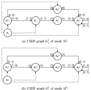
Fig. 1. An example of MADF graph (G1).

parameters, namely periodT and earliest starting timeS, where the deadline of the task is equal to its period (i.e., implicit deadline). The minimum periodTi [14] of any actor Ai∈ A

under SPS can be computed as:

Ti= lcm(~q)

qi

_maxA

i∈A{µiqi}

lcm(~q)

, (2)

where qi is the number of repetitions of actor Ai per graph

iteration, andµi is the worst-case execution time (WCET) of

actor Ai. In general, the derived period vector T~ must satisfy

the condition q1T1 = q2T2 = · · ·= qnTn = H, where H is

the iteration period, also called hyper period, that represents the duration needed by the graph to complete one iteration. The minimum period of the sink actor for a CSDF graph determines the maximum throughout that this graph can achieve. In addition, the utilization of any actor Ai∈ A, denoted byui,

can be computed as ui=µi/Ti, where ui∈(0,1].

To sustain a strictly periodic execution with the period derived by Equation (2), the earliest starting time Si [14]

of any actor Ai∈ A can be obtained as:

Si=       

0 i f prec(Ai)=∅

maxAj∈prec(Ai)(Sj→i) otherwise,

(3)

where prec(Ai) represents the set of predecessor actors of Ai

andSj→iis given by:

Sj→i= min t∈[0,Sj+H]

n

t: Prd

[Sj,max{Sj,t}+k) (Aj,Eu)

≥ Cns [t,max{Sj,t}+k]

(Ai,Eu), ∀k∈[0,H],k∈No

(4)

where Prd[ts,te)(Aj,Eu) is the total number of tokens pro-duced by Aj to edge Eu during the time interval [ts,te) and

Cns[ts,te](Ai,Eu) is the total number of tokens consumed byAi from edge Eu during the time interval [ts,te]. Equation (4)

considers the dependency between actors Aj and Ai, over

directed channel Eu. It calculates the earliest starting time Sj→i such that Ai is never blocked on reading data tokens

from Eu during its periodic execution. This is ensured by

checking that at each time instant, actor Ai can be fired such

that the cumulative number of tokens produced by Ajover Eu

is greater than or equal to the number of tokens Aiconsumes

from Eu. Start timesSj→i are computed for each actor Aj in

the predecessor set of Ai, i.e., Aj∈prec(Ai). Then, when actor Ai has several predecessors, the earliest starting time Si has

to be set to the maximum of starting times Sj→i considering

each predecessor in isolation, as captured by Equation (3). For more details, we refer the reader to [14].

A11 [1, 0] _A21 [1, 1] _A31 [2, 0] _A51

Ac

[0, 1] [1, 0] [1, 1]

A41 [0] [0]

[1] [1]

[0, 0] [0, 0]

(a) CSDF graphG1₁ of modeSI1.

A12 [1, 0] A22 A32 A52

A42

[0, 1] [1, 0] [0, 1]

Ac

[0, 1] [1, 0]

[1] [1]

[1] [1]

[1] [1]

(b) CSDF graphG2₁of modeSI2.

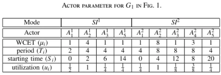
Fig. 2. Two modes of the MADF graph in Fig. 1.

IV. Mode-AwareDataFlow(MADF)

In this section, we introduce our new MoC called Mode-Aware Data Flow (MADF). MADF can capture multiple modes associated with an adaptive streaming application, where each individual mode is a CSDF graph [3]. Details and formal definitions of the MADF model and its operational semantics are given later in this section. Here, we explain the MADF intuitively by an example. Throughout this paper, we use graph

G1 shown in Fig. 1 as the running example to illustrate the definition of MADF and the hard real-time scheduling analysis related to MADF. This graph consists of 5 computation actors

A1 to A5 that communicate data over edges E1 to E5. Also, there is an extra actorAcwhich controls the switching between

modes through control edges E11, E22, E44, and E55 at run-time. Each edge contains a production and a consumption pattern, and some of these production and consumption patterns are parameterized. Having different values of parameters and worst-case execution times (WCET) of the actors determine different modes. For example, to specify the consumption pattern with variable length on edge E1 in graph G1, the parameterized notation [p2[1]] is used on edge E1 that is interpreted as a sequence of p2 elements with integer value 1, e.g., [2[1]]=[1,1]. Similarly, the notation [1[p4]] on edgeE4 is interpreted as a sequence of 1 element with integer value

p4, e.g., [1[2]]=[2]. Assume in this particular example that parameter vector (p1,p2,p4,p5,p6) can take only two values (0, 2, 0, 2, 0) and (1, 1, 1, 1, 1). Then, Ac can switch the

application between two corresponding modesSI1 and SI2 by setting the parameter vector to value (0, 2, 0, 2, 0) and (1, 1, 1, 1, 1), respectively, at run-time. Fig. 2(a) and (b) show the corresponding CSDF graphs of modeSI1 andSI2.

A. Formal Definition of MADF

Definition 1 (Mode-Aware Data Flow (MADF)).

TABLE I

Mapping relationM2for actorA2

inFig. 1.

~

p2=[p2] φ C¯2

2 2 [c1,c2]

1 1 [c3]

TABLE II

FunctionMC5defined for actor

A5inFig. 1.

S _N2

SI1 _[2,0]

SI2 _[1,1]

• A={A₁, . . . ,A_|A|}is a set of dataflow actors;

• Ac is the control actor to determine modes and their

transitions;

• E is the set of edges for data/parameter transfer;

• Π ={~p1, . . . , ~p|A|}is the set of parameter vectors, where

each ~pi∈Πis associated with a dataflow actor Ai.

For G1, A = {A1,A2,A3,A4,A5} is the set

of dataflow actors. Ac is the control actor.

E = {E1,E2,E3,E4,E5,E6,E11,E22,E44,E55} is the set of edges. For actor A5, ~p5=[p5,p6] is the parameter vector. The input port IP1 of actor A5 has a consumption sequence [1[p5],1[0]], which can be interpreted as [p5,0].

Definition 2(Dataflow Actor).A dataflow actor Aiis described

by a tuple (Ii, ICi, Oi,Ci,Mi), where

• I_i={IP1, . . . ,IP|Ii|}is the set of data input ports of actor

Ai;

• ICi is the control input port that reads parameter vector ~

pi for actor Ai;

• Oi={OP1, . . . ,OP|Oi|}is the set of data output ports of

actor Ai;

• Ci={c1, . . . ,c|C|}is the set of computations. When actor

Ai fires, it performs a computation ck∈ Ci;

• Mi : ~pi→ {φ,C¯i} is a mapping relation, where ~pi∈Π,

φ ∈ _N+, and C¯i ⊆ Ci is a sequence of computations

[ ¯Ci(1), . . . ,C¯i(k), . . . ,C¯i(φ)]withC¯i(k)∈ Ci,1≤k≤φ.

Actor A2 in Fig. 1 has a set of one input portI2={IP1}, a set of one output port O2={OP1} as well as a control input port IC2. A set of computationsC2={c1,c2,c3}is associated withA2. The mapping relationM2is given in Table I. It can be interpreted as follows: If p2 =2, actorA2repetitively performs computations according to sequence ¯C2=[c1,c2] every time when firingA2. When p2 =1, firing A2 performs computation

c3.

Definition 3(Control Actor). The control actor Acis described

by a tuple (IC,O_c,S,M_c), where

• S ={SI1, . . . ,SI|S|} is a set of mode identifiers, each of

which specifies a unique mode;

• IC is the control input port which is connected to the

external environment. Mode identifiers are read through the control input port from the environment;

• Oc ={OC1, . . . ,OC|A|} is a set of control output ports.

Parameter vector~piis sent through OCi∈ Oc to actor Ai;

• M_c={MC1, . . . ,MC|A|}is a set of functions defined for

each actor Ai∈ A. For each MCi∈ Mc, MCi : S →N|~pi|

is a function that takes a mode identifier and outputs a vector of non-negative integer values.

ForG1in Fig. 1, we have two mode identifiersS={SI1,SI2}. At run-time, control actor Ac reads these mode identifiers

through control port IC (black dot in Fig. 1). For actor A5,

MC5∈ Mc is given in Table II. As explained previously, the

parameter vector for actorA5 is ~p5=[p5,p6]. Therefore,MC5 takes a mode identifier and outputs a 2-dimensional vector as shown in the second column in Table II. For instance, mode

SI1 results in a non-negative integer vector [2,0].

To further define production/consumption sequences with variable length, we use the notationn[m] for a sequence ofn

elements with integer valuem, i.e.,

n[m]=[

ntimes

z }| {

m, . . . ,m].

Definition 4 (Input Port). An input port IP of an actor is

described by a tuple (CNS, MIP), where

• CNS = [φ₁[cns₁], . . . , φ_K[cns_K]] is the consumption

se-quence with φ phases, where φ = PK

i=1φi is deter-mined by the mapping relation M in Definition 2, and

cns1, . . . ,cnsK ∈N;

• MIP : ~pi→ψIP is a mapping relation, where~pi∈Πand

ψIP={φ1, . . . , φK,cns1, . . . ,cnsK}. (5)

Definition 5 (Output Port). An output port OP of an actor is

described by a tuple (PRD,MOP), where

• PRD = [φ1[prd1], . . . , φK[prdK]] is the production

se-quence with φ phases, where φ = PK

i=1φi is deter-mined by the mapping relation M in Definition 2, and

prd₁, . . . ,prd_K∈_N.

• MOP : ~pi→ψOP is mapping relation, where ~pi∈Πand

ψOP={φ1, . . . , φK,prd1, . . . ,prdK}. (6)

The consumption/production sequence defined here is a generalization of that for the CSDF MoC (see Section III-B). We can see that a CSDF actor has a constantφ phases in its consumption/production sequences, whereas the length of the phase of an MADF actor is parameterized byφ=PK

i=1φi. In

addition, the mapping relation MIP/MOP must be provided by

the application designer. Consider the two input portsIP1 and

IP2of actorA5in Fig. 1. The mapping relationsMIP1 andMIP2

are represented as follows:

MIP1 : ~p5 =[p5,p6]→ψIP1 ={φ1, φ2,cns1,cns2}={1,1,p5,0},

(7)

MIP2 : ~p5 =[p5,p6]→ψIP2 ={φ1, φ2,cns1,cns2}={1,1,0,p6}.

(8) It can be seen that parameter p5 is mapped to cns1 of IP1, parameter p6 is mapped tocns2 ofIP2, andφ1 and φ2 both are constant equal to 1. Therefore, the consumption sequence ofIP1 is CNS =[1[p5],1[0]] =[p5,0] and the consumption sequence of IP2 is CNS = [1[0],1[p6]] = [0,p6]. Similarly considering output portOP1 of actor A4, its mapping relation

MOP1 is given as:

MOP1 : ~p4=[p4]→ψOP1={φ1,prd1}={1,p4}. (9)

In this case, parameter p4 is mapped to prd1 and φ1 = 1. Therefore, production sequence PRD = [1[p4]] = [p4] is obtained forOP1 of A4.

Definition 6 (Edge). An edge E ∈ E is defined by a tuple

(Ai,OP),(Aj,IP)

Actors

5 10 15 SI1

L1 H1

S21

S31

S51 _Time

A11

A21

A31

A41

A51

20 H1

H1

H1

(a) ModeSI1in Fig. 2(a).

Actors

5 10 15

SI2

L2

S22

S32

S42

S52 _Time

A22

A12

A32

A42

A52

20

H2

H2

H2

H2

H2

(b) ModeSI2in Fig. 2(b).

Fig. 3. Execution of two iterations of both modesSI1_andSI2_{under self-timed}

scheduling.

• actor Ai produces a parameterized number of tokens to

edge E through output port OP;

• actor Ajconsumes a parameterized number of tokens from

E through input port IP.

Considering edge E5 in Fig. 1, it connects output port OP1 of actor A4 to input portIP2 of actor A5.

Definition 7 (Mode of MADF). A mode SIi of MADF is a

consistent and live CSDF graph, denoted as Gi_{, obtained by}

setting values of Πin Definition 1 as follows:

∀~pk∈Π : ~pk=MCk(SIi), (10)

where function MCk is given in Definition 3.

Definition 8(Mode of MADF Actor). An actor Akin mode SIi,

denoted by Ai

k, is a CSDF actor obtained from Ak as follows: ~

pk=MCk(SIi). (11)

Fig. 2(a) shows the CSDF graph of mode SI1 and Fig. 2(b) shows the CSDF graph of mode SI2. Consider function MC5 for actor A5 in Table II with parameter vector ~p5 =[p5,p6]. For instance, mode SI1 results in ~p5 =[p5,p6]=[2,0], where parameter values p5=2 and p6 =0. Consequently, according to mapping relations MIP1 and MIP2 given in Equation (7) and

Equation (8),cns1= p5=2 can be obtained for input portIP1 and cns2=p6=0 forIP2. This determines actorA1₅ shown in Fig. 2(a) for mode SI1.

Definition 9 (Inactive Actor). An MADF actor Ak_i is inactive

in mode SIk if the following conditions hold:

1) ∀IP∈ I_i : CNS=[0, . . . ,0];

2) ∀OP∈ O_i : PRD=[0, . . . ,0].

Otherwise, Ak

i is called active in mode SI k_.

For actor A1

4 shown in Fig. 2(a), it has consumption and production sequence [0]. Therefore, actor A4 is said to be inactive in mode SI1.

B. Operational Semantics

During execution of a MADF graph, it can be either in a steady-state or mode transition.

Definition 10 (Steady-state). A MADF graph is in a

steady-state of a mode SIi, if it satisfies Equation(10)with the same SIifor all its actors.

TABLE III

Actor parameter forG1inFig. 1.

Mode SI1 SI2

Actor A1

1 A12 A13 A15 A 2

1 A22 A23 A24 A25

WCET (µi) 1 4 1 1 1 8 1 3 1

period (Ti) 2 4 4 4 4 8 8 8 4

starting time (Si) 0 2 6 14 0 4 12 8 20

utilization (ui) 1₂ 1 1_{4 4}1 1₄ 1 1₈ 3₈ 1₄

Definition 11(Mode Transition). A MADF graph is in a mode

transition from mode SIo to SIl, where o,l, if some actors

have SIo for Equation(11) and the remaining active actors

have SIl for Equation(11).

In the steady-state of a MADF graph, all active actors execute in the same mode. As defined previously in Definition 7 and shown in Fig. 2(a) and Fig. 2(b), the steady-state of the MADF graph has the same operational semantics as a CSDF graph. We use hAk

i,xi to denote the x-th firing of actor Ai in mode SIk. AthAk

i,xi, it executes computation ¯Ci ((x−1) modφ)+

1_{, where ¯C}

i is given in Definition 2. The number of tokens

consumed and produced are specified according to Definitions 4 and 5, respectively. For instance, thex-th firing ofAk

i produces PRD((x−1) modφ)+1_{tokens through an output portOP. In}

each modeSIk, the MADF graph is a consistent and live CSDF graph and thus has the notion of graph iterations with a non-trivial repetition vector~qk∈_N|A| _{resulting from Equation (1).}

Next, we further define mode iterations.

Definition 12(Mode Iteration). One iteration Itk of a MADF

graph in mode SIk _{consists of one firing of control actor A}

c and qk

i ∈~q

k _{firings of each MADF actor A}k

i.

Consider the two modes shown in Fig. 2(a) and Fig. 2(b). Repetition vectors~q1 _and~q2 _are:

~

q1=[4,2,2,0,2], ~q2=[2,1,1,1,2]. (12) For any mode of a MADF graph, i.e., a live CSDF graph, underanyvalid schedule, it has (eventually) periodic execution in time. This holds for CSDF graphs under self-timed schedule [17], K-periodic schedule [18], and SPS [14]. The length of the periodic execution, callediteration period, determines the minimum time interval to complete one graph iteration (cf. Definition 12). The iteration period, denoted by

Hk, is equal for any actor in the same mode SIk. During a periodic execution, the starting time of each actor Ak_i, denoted bySk_i, indicates the time distance between the start of source actorAk

srcand the start of actorAki in the same iteration period.

Based on the notion of starting times, we define iteration

latency Lk _{of a MADF graph in modeSI}k _{as follows:}

Lk=Sk_snk−S_srck , (13)

whereSk

snk andS

k

Actors

A1

A2

A3

A5

5 10 15

A4

20 25 30 35 40 Time

L1 _Δ1→2_=L2

Δ2→1

Quiescent points for A1 _t MCR2 tMCR1

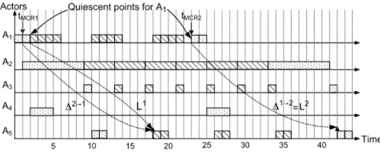
Fig. 4. An execution ofG1 in Fig. 1 with two mode transitions under the

ST transition protocol.MCR1at timetMCR1 denotes a transition request from

modeSI2 toSI1, andMCR2at timetMCR2denotes a transition request from

modeSI1 toSI2.

we obtain iteration latenciesL1 _=S1 5−S

1

1=10−0=10 and

L2_=S2 5−S

2

1=10−0=10 as shown in Fig. 3.

C. Mode Transition

While the operational semantics of a MADF graph in steady-state are the same as that of a CSDF graph, the transition of MADF graph from one mode to another is the crucial part that makes it fundamentally different from CSDF. The protocol for mode transitions has strong impact on the compile-time analyzability and implementation efficiency. In this section, we propose a novel and efficient protocol of mode transitions for MADF graphs.

During execution of a MADF graph, mode transitions may be triggered at run-time by receiving a Mode Change Request (MCR) from the external environment. We first assume that a MCR can be only accepted in the steady-state of a MADF graph, not in an ongoing mode transition. This means that any MCR occurred during an ongoing mode transition will be ignored. Consider a mode transition from SIo toSIl. The transition is accomplished by the control actor reading mode identifier SIl from its control input port (see the black dot in Fig. 1) and writing parameter values of ~pi to the control

output port connected to each dataflow actor Al

i according

to function MCi given in Definition 3. Then, Al_i reads new

parameter values ~pi from its control input port and sets the

sequence of computations according to mapping relation Mi

in Definition 2. The production and consumption sequences are obtained in accordance with MIP and MOP in Definition 4

and Definition 5, respectively. We further define/require that mode transitions are only allowed at quiescent points [19].

Definition 13 (Quiescent Point of MADF). For mode SIl, a

quiescent point of MADF actor Ai is firing hAli,xi in mode iteration Itl _{that satisfies}

¬∃hAl_i,yi ∈Itl : y<x. (14)

Definition 13 simply refers to the first firing of actor Ai

in each iteration Itl of mode SIl. Recall that each iteration of mode SIl consists of ql

i firings of actor Ai. Therefore, our

requirement that a mode transition is only allowed at a quiescent point implies that a transition from mode SIl to SIo of actor

Ai happens when all firings of actor Ai are completed in the

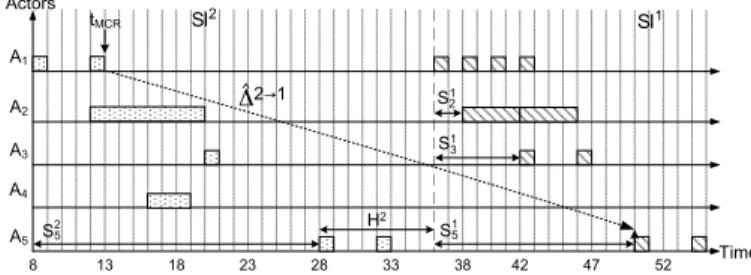
iteration of SIl when MCR occurs. Fig. 4 shows an execution ofG1 in Fig. 1 with two mode transitions. For instance, the

MCR at timetMCR1 =1 denotes a transition request from mode

SI2 toSI1. The mode transition of actorA1 happens when all firings of actorA1 are completed, that is at time 2 in Fig. 4 in this particular example.

Definition 13 defines mode transitions of MADF graphs as partially ordered actor firings. However, it does not specify at which time instance a mode transition actually starts. Therefore, below, we focus on the transition protocol that defines the points in time for occurrences of mode transitions. To quantify the transition protocol, we introduce a metric, called transition

delay, to measure the responsiveness of a protocol to a MCR.

Definition 14 (Transition Delay). For a MCR at time tMCR

calling for a mode transition from mode SIoto SIl, the transition

delay ∆o→l _{of a MADF graph is defined as}

∆o→l_=σo→l

snk −tMCR, (15)

whereσo_snk→l is the earliest starting time of the sink actor in the new mode SIl.

In Fig. 4, we can compute the transition delay for MCR1

occurred at timetMCR1 =1 as ∆2→1=18−1=17.

1) Self-timed Transition Protocol: In the existing adaptive

MoCs like FSM-SADF [5], a protocol, referred here as

Self-Timed (ST) transition protocol, is adopted. The ST protocol

specifies that actors are scheduled in the self-timed manner not only in the steady-state, but also during a mode transition. For FSM-SADF upon a MCR, a firing of a FSM-SADF actor in the new mode can start immediately after the firing of the actor completes the old mode iteration. The only possible delay is introduced due to availability of input data. One reason behind the ST protocol is that the ST schedule for a (C)SDF graph (steady-state of FSM-SADF1_{) leads to its highest achievable} throughput. However, the ST protocol generally introduces interference of one mode execution with another one. The time needed to complete mode transitions also fluctuates as the transition delay of an ongoing transition depends on the transitions that occurred in the past. We consider this as an undesired effect because mode transitions using the ST protocol become potentially slow and unpredictable. Another consequence of the incurred interference between modes using the ST transition protocol is the high time complexity of analyzing transition delays, because transition delays cannot be analyzed independently for each mode transition. The analysis proposed in [5] uses an approach based on state-space exploration, which has the exponential time complexity.

Consider G1 in Fig. 1 and an execution of G1 with the two mode transitions illustrated in Fig. 4. The execution is assumed under the ST schedule for both steady-state and mode transitions of G1. After MCR1 at time tMCR1, the transition from modeSI2 toSI1 introduces interference to execution of the new modeSI1 from execution of the old mode SI2. The interference increases the iteration latency of the new mode

SI1 toL1=S1₅−S1₁=18−2=16 from initially 10 as shown in Fig. 3(a) whenG1 is only executed in the steady-state of

1_{The steady-state of SADF is defined similarly to that of MADF. The only}

Actors

A12

5 10 15

S22

S52

S32

S31

S51

Time H2

H2

H1

S21

H1

H1

H2

H1

H2

A11

A22

A21

A32

A31

A52

A51

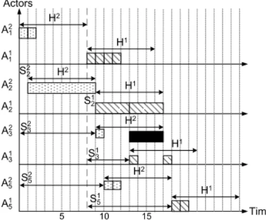
Fig. 5. An illustration of the Maximum-Overlap Offset (MOO) calculation.

modeSI1. Even worse, the interference is further propagated to the second mode transition after MCR2at timetMCR2. In this case, the iteration latency L2 =S₅2−S2₁ =42−23=19 is increased from initially 10 as shown in Fig. 3(b) when

G1 is only executed in the steady-state of mode SI2. This example thus clearly shows the problem of the ST protocol. That is, it introduces interference between the old and new modes due to mode transitions, thereby increasing the iteration latency of the new mode in the steady-state after the transition. Furthermore, the increase of iteration latency also potentially increases transition delays as it will be shown in the next section.

2) Maximum-Overlap Offset Transition Protocol: To address

the problem of the ST transition protocol explained above, we propose a new transition protocol, called Maximum-Overlap Offset(MOO).

Definition 15 (Maximum-Overlap Offset (MOO)). For a

MADF graph and a transition from mode SIo to SIl,

Maximum-Overlap Offset (MOO), denoted by x, is defined as

x=

      

maxAi∈Ao∩Al(S

o i −S

l

i) if maxAi∈Ao∩Al(S

o i −S

l i)>0

0 otherwise,

(16)

where Ao_{∩ A}l _{is set of actors active in both modes SI}o _and SIl_.

Basically, we first assume that the new mode SIl starts immediately after the source actor Ao

src of the old mode SI

o

completes its last iteration Ito. All actorsAl

i of the new mode

execute according to the earliest starting timesSl

iand iteration

period Hl in the steady-state. Under this assumption, if the execution of the new mode overlaps with the execution of the old mode in terms of iteration periodsHoandHl, we then need to offset the starting time of the new mode by the maximum overlap among all actors. In this way, the execution of the new mode will have the same iteration latency as that of the new mode in the steady-state, i.e., no interference between the execution of both old and new modes.

Consider MCR1at timetMCR1 shown in Fig. 4. Obtaining MOO xis illustrated in Fig. 5. We first assume that the new modeSI1starts at the time when the source actorA2₁ completes the last iteration at time 8 (see bold, dashed line in Fig. 5). Actors A1_i in the new mode start as if they executed in the

Actors

A1

A2

A3

A5

5 10 15

A4

20 25 30

x=4

35 Time

L1 L2

Start of mode SI1

H2 _H1

Start of mode SI2

Δ2→1 Δ1→2

tMCR1 tMCR2

Fig. 6. The execution ofG1 with two mode transitions under

Maximum-Overlap Offset (MOO) protocol.

steady-state of modeSI1. Then, we can see that, for actorA3, the execution ofA1

3in the new modeSI

1_{according toS}1

3in Fig. 3(a) overlaps 4 time units (solid bar in Fig. 5) with the execution ofA2

3in the old modeSI

2_{in terms of iteration periods H}2_and

H1_{. This is also the maximum overlap between the execution} of actors in modesSI2 and SI1. According to Definition 15, x

can be obtained through the following equations:

S2₁−S1₁ =0−0=0, S2₂−S1₂=1−1=0,

S2₃−S1₃ =9−5=4, S2₅−S1₅=10−10=0. Therefore, it results in an offset x = max(0,0,4,0) = 4 to the start of mode SI1 and is shown in Fig. 6. The starting time of the new modeSI1, namely the source actorA1

1, must be first delayed to the time when A1

2 completes the iteration period H2 _{in the last iteration, namely time 8 shown as the} first bold dashed line in Fig. 6. In addition, the MOO x=4 must be further added to the starting time of A1

1 (the second bold dashed line in Fig. 6). Fig. 6 also shows another transition from modeSI1toSI2with a MCR occurred at timetMCR2=23. The starting time of the source actorA2₁ in the new modeSI2

must be first delayed to the time 28 (the third bold dashed line in Fig. 6), namely the time when A1₁ completes the last iteration in the old modeSI1. To calculate the MOO xfor this transition, the following equations hold:

S1₁−S2₁=0−0=0, S1₂−S2₂=1−1=0,

S1₃−S2₃=5−9=−4, S1₅−S2₅=10−10=0. Thus, the equations above result in x=max(0,0,−4,0)=0. For this transition, the new modeSI2starts at time 28 as shown in Fig. 6.

The MOO protocol offers several advantages over the ST protocol. Essentially, the MOO protocol retains the iteration latency of the MADF graph in the new mode the same as the initial value, thereby avoiding the interference between the old and new modes. For instance, afterMCR1andMCR2in Fig. 6, modeSI1 andSI2 still have the initial iteration latency

Concerning the transition delay, it may be the case that the MOO protocol results in initially longer transition delay than the ST protocol does due to the offset given in Definition 15. ForMCR1occurred at time tMCR1, the transition delay of the MOO protocol is ∆2→1 _{= 22−1 = 21 as shown in Fig. 6,} whereas the transition delay of the ST protocol is equal to

∆2→1 _{=18−1=17 as shown in Fig. 4. On the other hand,} let us consider the same transition requestMCR2 occurred at time tMCR2 =23 shown in Fig. 4 and Fig. 6. ForMCR2, the ST protocol results in transition delay ∆1→2_{=42−23=19 as} shown in Fig. 4. In contrast, the transition delay for the MOO protocol is∆1→2=38−23=16 as shown in Fig. 6. The MOO protocol could provide shorter transition delay than the ST protocol, thereby faster responsiveness to a mode transition.

V. HardReal-TimeAnalysis andScheduling ofMADF

Based on the proposed MOO protocol for mode transitions, in this section, we propose a hard real-time analysis and scheduling framework for MADF. More specifically, we propose an analysis technique for mode transitions in MADF to reason about transition delays, such that timing constraints can be guaranteed. The hard real-time scheduling framework for MADF graphs is an extension of the SPS [14] framework initially developed for CSDF graphs.

As explained in Section III-C, the key concept of the SPS framework is to derive a periodic taskset representation for a CSDF graph. Since the steady-state of a mode can be considered as a CSDF graph according to Definitions 7 and 10, it is thus straightforward to represent the steady-state of a MADF graph as a periodic taskset and schedule the resulting taskset using any well-known hard real-time scheduling algorithm. Using the SPS framework, we can derive the two main parameters for each MADF actor in mode SIk, namely the period (Tk

i in

Equation (2)) and the earliest starting time (Sk

i in Equation (3)).

Under SPS, the iteration period in mode SIk is obtained as

Hk _=qk iT

k i, ∃A

k

i ∈ A. Below, we focus on determining the

earliest starting time of each actor in the new mode upon a transition. From the earliest starting time, we can reason about the transition delay to quantify the responsiveness of a transition.

Upon a MCR, a MADF graph can safely switch to the new mode if all of its actors have completed their last iteration in the old mode upon synchronous protocol. In this case, the firings of MADF actors in the new mode do not overlap with the firings of actors in the old mode. This is called synchronous protocol [12] in real-time systems with mode change. One of its advantages is the simplicity, i.e., the synchronous protocol does not require any schedulability test at both compile-time and run-time. However, other protocols lead to earlier starting times than the synchronous protocol. Therefore, the synchronous protocol sets an upper bound on the earliest starting time for each MADF actor in the new mode.

Lemma 1. For a MADF graph G under SPS and a MCR from

mode SIo to SIlat time tMCR, the earliest starting time of actor Al_i,σˆo_i→l, is upper bounded by

ˆ

σo→l

i =F

o src+S

o snk+S

l

i, (17)

Actors

A1

A2

A3

A5

A4

SI2 _SI1

H2

8 13 18 23 28 33 38 42 47 52 Time

Δ2→1

⌃ _S

21

S31

S51

S52

tMCR

Fig. 7. Upper bounds of earliest starting times for transition from modeSI2

toSI1.

where Fo

src indicates the time when the source actor Aosrc

completes its last iteration Ito of the old mode SIo and is

given by

F_srco =t_So+

t_MCR−to S Ho

Ho. (18)

to

S is the starting time of mode SI

o _{and H}o _{is the iteration} period of mode SIo.

Proof. As explained previously for a transition from modeSIo

toSIl, the upper bound of the earliest starting time for each actor Al_i is computed in such a way that no firings of actors

Ao_i and Al_i occur simultaneously. This means, the start of an actor Al_i must be later than all actors Ao_i have completed the last iteration Ito _{of the old mode SI}o_{. Given that mode SI}o

starts at time to

S, the completion time of all actorsA o i in the

last iterationIto can be thus computed as

Fo_snk=to_S +

t_MCR−to S Ho

Ho+So_snk+Ho. (19)

where Fo

snk is the time when the old modeSI

o _{completes the}

last iterationIto. It is assumed that the sink actorAo_snk is the last actor to complete the iteration, i.e.,∀Ao_i ∈ A,So_i ≤So_snk. Given Equation (18), Equation (19) can be rewritten as

Fo_snk=to_S +

t_MCR−to S Ho

Ho+So_snk=Fo_src+So_snk.

Now, starting the source actorAl

src at any time later than Fsnko is valid without introducing simultaneous execution of actors

Ao

i andA

l

i. Therefore, the earliest starting time of source actor Al

src is ˆσosrc→l = Fsnko . For any actor A

l

i ∈ A \A l

src, its earliest starting times must satisfy Equation (3) imposed by the SPS framework. That is, the earliest starting time ˆσo→l

i of actor A l i

can be obtained by addingSl i to ˆσ

o→l

src .

Let us consider the actor parameters given in Table III forG1 in Fig. 1. The third row shows the WCET for each actor in modes SI1 and SI2. Based on WCETs, the period (fourth row in Table III) and the earliest starting time (fifth row in Table III) for each actor in the steady-state of both modes are obtained according to Equation (2) and Equation (3), respectively. Given~q2 _{in Equation (12), we can also compute} iteration period H2 _{= q}2

1T 2

1 = 2×4= 8. Now consider the mode transition from modeSI2toSI1shown in Fig. 7. Assume that the MCR occurs at timetMCR =13 and modeSI2 starts at timet2_S =8. The completion time of the last iterationIt2 is equal to the completion time of the sink actor A2₅ computed as

F2_snk=t2_S +

t_MCR−t2 S H2

H2+S2₅=8+

₁₃₋₈

8

Actors

A1

A2

A3

A5 A4

SI1 SI2

8 13 18 23 28 33 38

x

Time

tMCR

S51 S31 S21

Fig. 8. Earliest starting times for transition from modeSI2 toSI1with the MOO protocol.

In Fig. 7, F2

snk corresponds to the earliest starting time of the source actor A1₁ (bold dashed line). Finally, we can compute the earliest starting time for each actor in the new modeSI1

by adding S1_i. Considering for instance the sink actor A1₅ in the new mode with S1₅ =14, the upper bound of its earliest starting time can be obtained as

ˆ

σ2→1

5 =F 2 src+S

2 5+S

1 5=F

2 snk+S

1

5=36+14=50. We can thus compute the transition delay (cf. Definition 14) as

ˆ

∆2→1_=σˆ2→1

5 −tMCR=50−13=37.

Although the upper bound of the earliest starting times is easy to obtain for MADF actors in the new mode, it does not provide a responsive mode transition. Therefore, here we aim at deriving a lower bound of the earliest starting times with the proposed MOO protocol.

Lemma 2. For a MADF graph under SPS and a MCR from

mode SIo _{to SI}l_{at time t}

MCR, the earliest starting time of actor Al

i using the MOO protocol is lower bounded byσˇ

o→l

i given

as

ˇ

σo→l

i =F

o

src+x+Sli, (20)

where Fo

src is given in Equation (18) and x is given in

Equation(16).

Proof. Under the MOO protocol, the start of actor Al_i must be later than the time when Ao_i, if any, completes its last iteration in the old modeSIo. We assume that the source actorAlsrcis the first actor to start in the new mode SIl_{, i.e.,∀A}l

i∈ A,S l i≥S

l

src. Thus, the starting time of the source actorAl

src is at least equal to the completion time of the last iteration of Ao

src, denoted by

Fo

src. Given Fosrc in Equation (18), it thus holds ˇσosrc→l ≥Fosrc. Then, the offset x because of the MOO protocol given in Equation (16) must be taken into account. Consequently, the earliest starting time ofAl

srcis lower bounded by ˇσo

→l

src =Fsrco +x. For any actor Al

i ∈ A \A l

src, its earliest starting times must satisfy Equation (3) imposed by the SPS framework. Hence, the earliest starting time ˇσo_i→l of actorAl_i can be obtained by

addingSl_i to ˇσosrc→l.

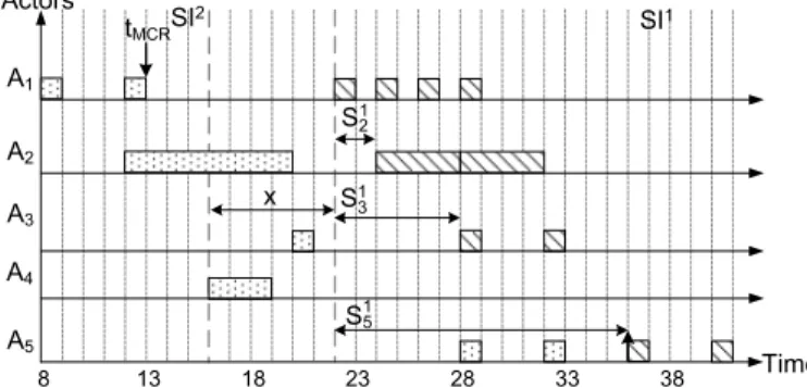
Let us consider again the transition from modeSI2 toSI1. With the MOO protocol, the mode transition is illustrated in Fig. 8. Upon the MCR at time tMCR=13 and t2_S =8, source

actorA2₁ completes its last iteration It2 in the old modeSI2 at the time (cf. Equation (18)) given as

Fsrc2 =F 2 1=t

2

S +

t_MCR−t2 S H2

H2=8+

₁₃₋₈

8

8=16.

This is the earliest possible time at which mode transition

is allowed. For MOO, x can be computed according to

Equation (16). Therefore, the following equations hold:

S2₁−S1₁=0−0=0, S2₂−S1₂ =4−2=2,

S2₃−S1₃=12−6=6, S2₅−S1₅=20−14=6. It thus yields x=max(0,2,6,6)=6, i.e., an offset x=6 is added to Fsrc2 . It can be seen in Fig. 8 that the source actorA11 starts at timeFsrc2 +x=16+6=22. Finally, the earliest starting times of actors in modeSI1 can be determined by adding S1

i.

Considering for instanceA1

5 in the new mode, the lower bound of its earliest starting time can be obtained as:

ˇ

σ2→1

5 =F 2

src+x+S15=16+6+14=36.

Now, the transition delay (cf. Definition 14) can be obtained as

ˇ

∆2→1_=σˇ2→1

5 −tMCR=36−13=23.

A. Scheduling Analysis under a Fixed Allocation of Actors

During a mode transition of a MADF graph according to the MOO protocol, actors execute simultaneously in the old and new modes. The derived starting time in Lemma 2 for each actor is only the lower bound because the allocation of actors on PEs is not taken into account yet. That means, the derived starting times according to Lemma 2 can be only achieved during mode transitions when each actor is allocated to a separate PE. In a practical system where multiple actors are allocated to the same PE, the PE may be potentially overloaded during mode transitions. To avoid overloading of PEs, the earliest starting times of actors may be further delayed.

Lemma 3. For a MADF graph under SPS, a MCR from mode

SIo to SIl, and a m-partition of all actors Ψ ={Ψ₁, . . . ,Ψ_m}, where m is the number of PEs, the earliest starting time of an actor Al_i without overloading the underlying PE is given by

σo→l

i =F

o src+δ

o→l_+Sl

i, (21)

where F_srco is computed by Equation (18)andδo→lis obtained as

δo→l_{= min}

t∈[x,So snk]

{t:Uj(k)≤UB, ∀k∈[t,Sosnk]∧∀Ψj∈Ψ}. (22)

UB denotes the utilization bound of the scheduling algorithm

used to schedule actors on each PE. Ψj contains the set of

actors allocated to PEj. Uj(k) is the total utilization of PEj

at time k demanded by both mode SIo _{and SI}l_{actors, and is}

given by

Uj(k)= X

Ao d∈Ψj

uo_d−h(k−So_d)·uo_d

| {z } Uo

j(k)

+ X

Al

d∈Ψj

h(k−S_dl −t)·ul_d

| {z } Ul

j(k)

,

A1

A2

A3

A5

PE1 PE2

A4

Ac

PE3

Fig. 9. Allocation of all MADF actors in Fig. 1 to 3 PEs.

Ao

d∈Ψj is an actor active in the old mode SI

o _{and allocated}

to PEj. Al_d ∈Ψj is an actor active in the new mode SIl and allocated to PEj. h(t) is the Heaviside step function.

Proof. Lemma 2 shows the lower bound of the earliest starting

time for actor Al_i in the new modeSIl. However, starting Al_iat time ˇσo_i→lmay overload PEj, i.e., the resulting total utilization

of PEj, denoted byUj( ˇσoi→l), exceedsUB. Therefore, in this

case, the earliest starting timeσo→l

i must be delayed byδ

o→l

such that Uj(σoi→l) ≤ UB holds. From Equation (21) and

Equation (20), we can see that δo→l _{is lower bounded by x}

which corresponds to the MOO protocol. In addition, δo→l

is upper bounded by So

snk if we consider Equation (21) and Equation (17).

δo→l_{of interest is the minimum timetin the bounded interval}

[x,So_snk] that satisfies two conditions.

Condition 1: For each PEj, the total utilization cannot exceed UB at time t, i.e., Uj(t)≤UB. The total utilizationUj(t) in

Equation (23) consists of two parts, namely Uo

j(t) and U l j(t). Uo

j(t) denotes the PE capacity occupied by the actors in mode SIothat are not completed yet. Additional PE capacityUl_j(t) is demanded by the already released actors in the new mode SIl.

Condition 2: We need to check all time instantsk>tin the interval [t,So

snk], such thatUj(k)≤UB, to guarantee that each

PEj is not overloaded during the mode transition.

Fig. 9 shows all actors ofG1in Fig. 1 allocated to 3 PEs and let us assume that the actors allocated to each PE are scheduled using the EDF scheduling algorithm [16]. The utilization bound of EDF is given in [16] asUB=1. Given this allocation and the transition from mode SI2 to SI1 shown in Fig. 8, the lower bound of the earliest starting time ˇσ2→1

1 = 22 for actor A

1 1 cannot be achieved. At time 22, only actor A2

1 has completed the last iterationIt2 on PE1. Starting the new modeSI1 at time 22 corresponds toδ2→1_{=x=6. The total utilization of PE1} demanded by the actors in the old mode SI2 at time 22, i.e.,

U2

1(6), can be computed as follows:

U₁2(6)= X

A2

d∈Ψ1

u2_d−h(6−S2_d)·u2_d, d∈ {1,3,4,5}

=u2₁−h(6)·u2₁+u2₃−h(−6)·u2₃+u2₄−h(−2)·u2₄+u2₅−h(−14)·u2₅ =0+u2₃+u2₄+u2₅=1

8+ 3 8+

1 4=

3 4.

Enabling A1

1 in the new mode SI

1 _{at time 22 would yield}

U1(6)=U12(6)+u 1 1=

3 4+

1

2 >UB=1,

Actors

A1

A2

A3

A5 A4

8 13 18 23 28 33 38 42

x δ

SI1 SI2

Time tMCR

2→1

S21

S31

S51

Fig. 10. Earliest starting times for transitionSI2toSI1on 3 PEs shown in Fig. 9.

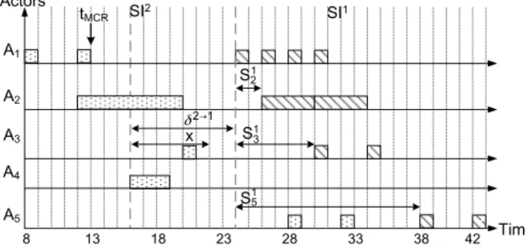
thereby leading to being unschedulable on PE1. In this case, the earliest starting times of all actors in mode SI1 must be delayed by δ2→1_{=8 to time 24 as shown in Fig. 10. At time} 24, the total utilization demanded by modeSI2 actors is

U2₁(8)= X

A2

d∈Ψ1

u2_d−h(8−S2_d)·u2_d, d∈ {1,3,4,5}

=u2₁−h(8)·u2₁+u2₃−h(−4)·u2₃+u2₄−h(0)·u2₄+u2₅−h(−12)·u2₅ =0+u2₃+0+u2₅=1

8+ 1 4=

3 8.

Now, enabling A1

1 in the new mode at time 24 results in the total utilization of PE1 as

U1(8)=U2₁(8)+u1₁= 3

8+ 1 2 <1.

Next, assuming that the new mode SI1 starts at time 24, we need to check that the remaining actors in the new mode

SI1, namely A1₃ andA₅1, can start with S₃1 andS1₅ respectively without overloading PE1. For instance, enablingA13 at time 24 results in starting timeσ2₃→1=24+S1₃=24+6=30. At time 30, the total utilization of PE1 can be obtained according to Equation (23) as follows:

U₁2(8+6)= X

A2

d∈Ψ1

u2_d−h(14−S2_d)·u2_d, d∈ {1,3,4,5}

=u2₁−h(14)·u2₁+u2₃−h(2)·u2₃+u2₄−h(6)·u2₄+u2₅−h(−6)·u2₅ =0+0+0+u2₅=1

4,

U₁1(8+6)= X

A1_d∈_Ψ1

h(14−S1_d−8)·u_d1, d∈ {1,3,5}

=h(6)u1₁+h(0)u₃1+h(−8)u1₅=1

2+ 1 4=

3 4,

U1(8+6)=U21(8+6)+U

1

1(8+6)=1=UB.

Hence, actors A2₅, A1₁, andA1₃ are schedulable on PE1 using EDF. Similarly, starting A1₅ at timeσ₅2→1=24+S1₅=38 still keeps the resulting set of actors schedulable on PE1.

Using Lemma 3, we can quantify the maximum and minimum transition delays for any transition from modeSIo

toSIl.

Theorem 2. For a MADF graph under SPS, a fixed allocation

of all MADF actorsΨ ={Ψ₁, . . . ,Ψ_m} to m PEs, and a MCR from mode SIoto SIl, the minimum transition delay is given by

∆o→l

min =δ

o→l_+Sl

snk (24)

and the maximum transition delay is given by

∆o→l

max =δ

o→l_+Sl snk+H

Read

Wave DFT AddCosWin Rec2Polar Unwrap

Spec2Env male2female

Polar2Rec InvDFT

Write Wave

Ac

IC

[1[128dl]]

[1[256]][1[256]] [128[dl]] [128[dl]] [128[dl]]

[1[256]] [1[256]] [1[128dl]] [128[dl]] [128[dl]] [128[dl]]

[128[dl]] [128[dl]]

[128[dl]] [128[dl]]

[128[dl]]

[128[dl]] [128[dl]]

[128[dl]]

[128[dl]] [128[dl]] [128[dl]]

[128[dl]]

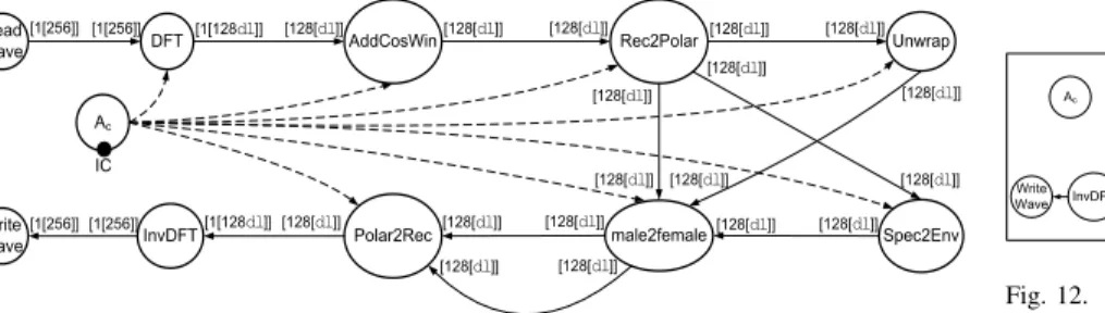
Fig. 11. MADF graph of Vocoder.

PE1 PE2

Read Wave

DFT

AddCosWin Rec2Polar Unwrap

Spec2Env male2female

Polar2Rec InvDFT Write Wave

PE3

PE4

Ac

Fig. 12. Allocation of dataflow actors of Vocoder to 4 PEs. The control edges are omitted to avoid cluttering.

where δo→l is computed by Lemma 3, Sl_snk is the starting time of the sink actor in the new mode SIl, and Ho is the iteration period of the old mode SIo.

Proof. For a MCR from modeSIo toSIl, the transition delay

∆o→l _{of a MADF graph is given in Definition 14 as ∆}o→l₌ σo→l

snk −tMCR, where the earliest starting time of the sink actor is calculated as σo_snk→l=Fosrc+δo→l+Slsnkaccording to Lemma 3. Therefore, ∆o→l _{can be rewritten as ∆}o→l _{= F}o

src+δo→l+

Sl

snk−tMCR. Essentially,∆o→l is composed of three parts. In the first part, the MOO transition protocol together with a fixed allocation of the MADF actors determine δo→l_{. The second}

partSl

snkresults from the SPS framework. These two parts thus can be determined at compile-time. The third part Fo

src−tMCR depends on when the MCR occurs, namely attMCR, which can only be determined at run-time. In the following, we distinguish two cases fortMCR:

Case 1: Assume that the MCR occurs at the end of an iteration of the source actor in the old modeSIo, i.e.,tMCR=

F_srco . Then, the source actor shall be only delayed by δo→l to start in the new modeSIl according to Lemma 3, thereby guaranteeing the fastest possible start of the new modeSIl. As a consequence, it results in the minimum possible transition delay. Therefore, substituting tMCR=Fosrc, we obtain

∆o→l

min =F

o

src+δ

o→l_+Sl

snk−F

o

src=δ

o→l_+Sl

snk. Case 2: Assume that the MCR occurs at the beginning of an iteration of the source actor in the old modeSIo_{, i.e.,t}

MCR=

Fo

src−Ho. Then, the source actor cannot start in the new mode before it completes the whole iteration in the old mode SIo

followed by the delay δo→l _{according to Lemma 3. Therefore,}

the maximum transition delay is computed as follows:

∆o→l

max =F

o

src+δ

o→l₊

Sl_snk−(Fsrco −H

o_)=δo→l₊

Sl_snk+Ho.

It can be seen from Theorem 2 that the maximum and minimum transition delays solely depend on the allocation of MADF actors and the old and new modes in question, irrespective of the previously occurred transitions. The old and new modes determineHo _andSl

snk, respectively, while the allocation of MADF actors determines the value ofδo→l_{. Here,}

the offset xdue to our MOO protocol is captured in δo→l _and

can be considered as performance overhead if x,0. The other

parts, namely Ho _{and S}l

snk, in the maximum and minimum transition delays cannot be avoided as they will be present in any transition protocol.

VI. CaseStudies

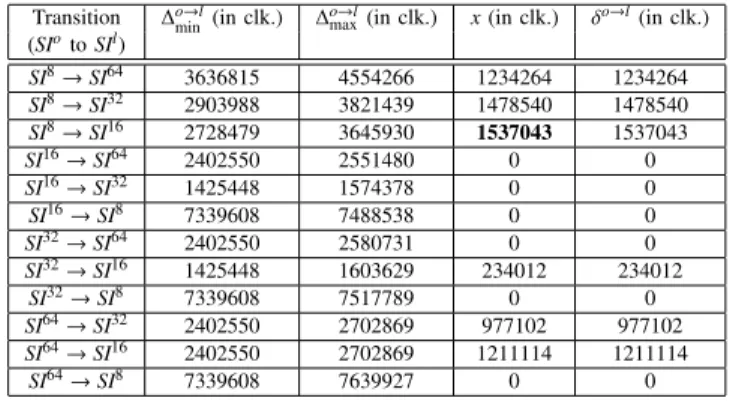
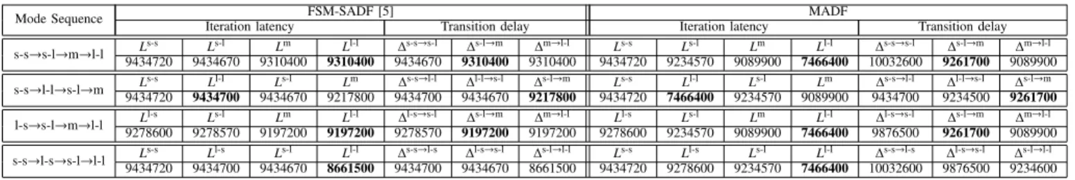
To evaluate our proposed MADF MoC and MOO protocol, in this section, we present two case studies. In the first case study, we model a real-life adaptive streaming application, called Vocoder, with our MADF MoC proposed in Section IV and apply the hard real-time analysis proposed in Section V. With this case study, we show that the MADF MoC is capable of capturing different application modes and the transitions between them. Then, in the second case study, we model another real-life adaptive streaming application, called MP3decoder, with MADF and we focus on analyzing the transition delays and demonstrating the effectiveness of our MADF model armed with the proposed MOO transition protocol compared to the well-known FSM-SADF model [5] which also can capture modes/scenarios. In this case study, we adopt self-timed scheduling for both our MADF and FSM-SADF models in the steady-state. The major difference between these models in this case study is their transition protocol which is the MOO protocol in our MADF model and the self-timed protocol in FSM-SADF. Another example of the application of our MOO protocol can be found in [20].

A. Case Study 1

In this section, we consider a real-life adaptive application from the StreamIT benchmark suit [21], called Vocoder, which implements a phase voice encoder and performs pitch transposition of recorded sounds from male to female. We modeled Vocoder using a MADF graph with 4 modes, which capture different workloads. The MADF graph of Vocoder is shown in Fig. 11. Depending on the desired quality of audio encoding and various performance requirements, the resource manager as a middle-ware or OS-like component for the MPSoC may switch between four different modes of Vocoder at run-time. The four modesS={SI8,SI16,SI32,SI64}specify different lengths of the Discrete Fourier Transform (DFT), denoted by dl∈ {8,16,32,64}. ModeSI8 (dl=8) requires the least amount of computation at the cost of the worst voice encoding quality among all DFT lengths. ModeSI64 (dl=64) produces the best quality of voice encoding among all modes, but is computationally intensive. The other two modesSI16and