Equation Section 1 First Draft: Do Not Quote

Equation Section 1

First Draft: Do Not Quote

Estimating Nonlinear Effects of

Management Styles in the US Equity Market

Dan diBartolomeo

Sandy Warrick, CFA

Northfield Information Services, Inc.

184 High Street, Boston, MA 02110

617 451 2222

617 451 2122 (fax)

[email protected]

[email protected]

Abstract

The vast majority of asset pricing models assume linear relationships between security returns and underlying factors. Among investment practitioners, models of both risk and return derived from such asset pricing models continue the assumption of linear

relationships.

In this paper, we report on an investment “style” scoring model of the US equity market that has been in practitioner use for over ten years. Returns associated with the style scores, their squares and interaction terms are investigated using both deciles analysis and via a monthly cross-sectional regression.

The style scores are shown to have a high degree of statistical significance in the cross-section of US stock returns from April of 1991 to March of 2001. Identifiable time series properties are found for the coefficients describing the linear relationships to the style scores.

Contrary to traditional models, return relationships are also shown for some of the second order and interaction effects for a large fraction of the cross-sections. These relationships appear to be both statistically and economically significant.

We conclude from this information that practitioners ought pay substantial attention to second order and interaction effects arising from active management “bets”. There is also evidence that second order and interaction effects have a meaningful role in asset pricing.

Introduction

The vast majority of asset pricing models assume linear relationships between security returns and underlying factors. Among investment practitioners, models of both risk and return derived from such asset pricing models continue the assumption of linear

relationships.

In most academic research, the factors underlying equity security behavior are

represented by observable characteristics such as capitalization, or the ratio of book value to market price. For some models, the metrics cannot be observed but most be

statistically estimated (e.g. market beta).

Within the practitioner community it is commonplace to characterize investment themes with qualitative titles such as “growth”, “value” or momentum. These qualitative titles may represent concepts that encompass several quantitative measures of the properties of equity securities.

In this paper, we report on an investment “style” scoring model of the US equity market that has been in practitioner use for over ten years. Returns associated with the style scores, their squares and interaction terms are investigated using both deciles analysis and via a monthly cross-sectional regression.

Unlike any previous literature, this paper studies the nonlinear behavior of stock returns in relationship to richly defined underlying factors that are consistent with the actual methodologies of the practitioner community.

Literature Review

There is an extremely rich literature in asset pricing models. Among the most notable are the Capital Asset Pricing Model of William Sharpe (1964) and the Arbitrage Pricing Theory of Ross (1976). These models suggest that financial markets operate efficiently, in an equilibrium state where expectations of returns are linearly related to some

underlying factors of risk.

These theoretical works have been followed by countless empirical studies. Notable works include Fama and MacBeth (1973), Reinganum (1981), Fama and French (1992), and Lakonishok, Schliefer and Vishny (1994). The members of this genre of papers provide evidence of market efficiency, or purport to illustrate some anomalous exception thereto.

Putting aside the issue of market efficiency, linear factor models have also achieved widespread acceptance as means of forecasting the correlation and covariance of

securities. Farrell (1976) provides an excellent overview of the use of multi-index models for estimation of risk. Rosenberg (1974) and Rosenberg and Guy (1976) investigate using fundamental variables rather than time series methods linear estimation of components of risk. Grinold (1993) provides an interesting synthesis. He suggests that while the

empirical evidence of market efficiency is mixed, there has been little challenge to usefulness of linear factor models in the estimation of risk.

There is an extensive literature regarding the nonlinear aspects of market index returns. In this area, we find papers such as Lebaron and Scheinkman (1989), Willey (1992) and Abhyankar, Copeland and Wong (1995). The principal empirical results of these papers revolve around higher order time-series behavior of market indices.

However, there are a very small number of papers that challenge the underlying assumptions of linear factor models. Elton and Gruber (1992) address the issue of a multi-index model with a nonnormal asset return distribution. Closest in intent to this paper is the work of Qi (1999), wherein nonlinear relationships between stock returns and underlying fundamental and economic variables are studied. Papers on the interaction between stock return factors include Quinton (2000) and Aggrawal, Johnson and Waggle (2001).

Investment “style” is a predominant consideration among investment practitioners, particularly active managers in equity markets. Practitioner investment strategies

normally involve the pursuit of a particular investment thesis (e.g. “value”, “momentum”, etc.) through targeting a number of purported desirable security (or portfolio)

characteristics. Among the more prominent papers on equity style are Estep (1987), Arnott, Dorian and Macedo (1992), Christopherson (1995) and Gallo and Lockwood (1997). The effect of style in international equity markets is reviewed in Arshanapalli, Coggin, Doukas and Shea (1998) and Michaud (1998).

Data

In 1989, Northfield Information Services studied the “style” issue by surveying several hundred US equity managers as to their approach to active portfolio management. Styles were identified based on the answers to two key questions:

1. What do you call your approach to stock selection?

2. In ten words or less, what is your approach to stock selection?

Based on the tabulation of these results, Northfield developed seven different equity style classifications.

1. Value 2. Growth

3. Price momentum

4. Sector momentum (Timeliness) 5. Safety first (capital preservation) 6. Economic forecasts

7. Market timing

Northfield choose to develop a style scoring method encompassing the first five styles listed above. The next step was to develop observable quantitative metrics from the short descriptions that managers had provided of their strategies. For example, a dividend

discount model might be a metric of a “value” strategy, while targeting low beta, low volatility securities would be a metric for “safety first” approach. In all, approximately forty of these descriptive metrics were developed to span the various views of the many managers as to their view of how to define and pursue their chosen style. Details of the descriptive metrics can be found in the Appendix.

The descriptive metrics are grouped into the five identified styles. Each month, Northfield ranks all US traded stocks (NYSE, AMEX and NASDAQ) on all of descriptive metrics. The ranking values are then averaged across all of the metrics within each of the styles to form a composite ranking for that style. As such, each stock has monthly ranking of how well it typifies the characteristics of stocks that would be consistent with a particular style. It should be noted that this scoring scheme is meant only to describe the likely affinity that various styles of manager would have for a particular stock, not to indicate in any way whether a particular stock was attractive or could be expected to offer extraordinary returns.

Each month-end since April of 1991, Northfield has produced this data set in a consistent fashion, and made it commercially available to the institutional investment community. As the database is free of both look-ahead and survivor bias, it is possible to perform studies of these data without worrying that any data snooping bias will be introduced due to the composition of the database.

Prior work related to this data set include Apt, diBartolomeo and Godfredsen (1993), wherein the Timeliness style score is developed and diBartolomeo (1996) where the time-series properties of the style returns is explored.

Hypothesis & Experimental Design

Our hypothesis is that nonlinear relationships exist between the style scores and US stock returns. To test this hypothesis, we will estimate a series of equations over the

information in our data set. The first equation will be the classic linear model: 5

i,t j,t i,j,t-1 i,t j = 1

R =

å

Where

Ri,t = return on security i during period t

Rj,t = return to style score j during period t

Ei,j,t-1 = value of style score j for security i at the end of period t-1

εi.t = return error term for security i during period t

We will then move to the heart of our analysis. We extend the model to include second order (j = k) and interaction terms (j <> k):

5 5 5

i,t j,t i,j,t-1 j,k,t i,j,t-1 i,k,t-1 i,t j = 1 j = 1 k = 1

R =

å

å å

Rj,k,t = return to interaction of style score j with style score k during period t

If we find that the coefficients representing returns to the style scores have a statistically significant time-series mean, this suggests that the particular term in question is important in the relationship between this form of risk characterization and expected returns. Any significant returns to non-linear would be considered to be violations of Arbitrage Pricing Theory, which posits that only linear relationships can exist between factors and returns, else it would be possible to create arbitrage (bullet vs. barbell) portfolios that would exploit the nonlinear relationship.

If the coefficients representing returns to the style scores have persistently high cross-sectional significance (high absolute value of the t-statistics), it suggests that this form of risk characterization is valuable in explaining the period-to-period variations in returns to stocks. Such a model is useful construct in describing the covariance among equity securities and portfolios thereof.

Given the previous work on the predictability of time-series aspects of returns to the style scores, we will also test the above equations with accounting for autoregressive

relationships in the resultant coefficients.

For simplicity of computation, all the security return values and the style score values used in the analysis were normalized into z-scores. As such, the coefficients arising out of the cross-sectional regressions represent partial correlation coefficients.

Discussion of Results

As is often done in empirical stock market research, we begin our investigation by doing a monthly sorting of the stock universe into deciles according to each of the five style scores. This analysis is done for each month from January of 1991 through March of 2001. By observing the returns of the deciles, and averaging the returns of each group over the one hundred and twenty six month periods, it is possible to develop considerable insight into linear and nonlinear relation between returns and factors. These average decile returns for each of the five factors are shown in Figure 1 through Figure 6.

Figure 1 shows that the Value style score shows that the highest quintile (the top two deciles, those with the most value) had a significantly higher average monthly return than the other quintiles. The top quintile has approximately 1% per month higher returns than the other fractiles.

The Growth style score is illustrated in Figure 2. Over the sample period, very little difference in return is evidenced between the various deciles.

Figure 3 shows that for Momentum style score, the lowest decile (those with the least momentum attributes) had a 90 basis point higher average monthly return than the other deciles, but the highest decile (those with the most greatest attributes) had the second highest returns. This highly nonlinear behavior may be able to be exploited.

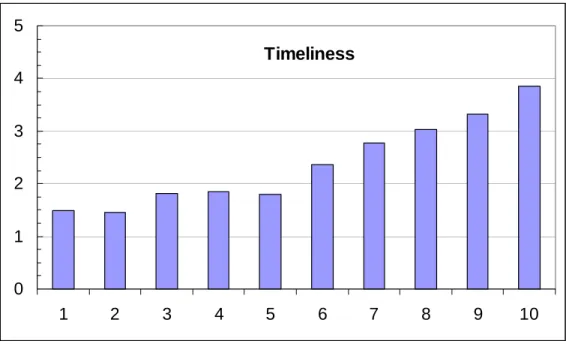
The Timeliness style score is presented Figure 4. It shows that the highest timeliness decile had a significantly higher average monthly return than the other deciles. This style score shows a high degree of monotonic behavior. The inter-decile spread is reasonably uniform, at approximately 60 b.p. per month premium per decile.

Figure 5 shows that the lowest decile of Safety First style scores (those with the least safety attributes) had a significantly higher average monthly return than the other deciles. As market beta is a large component of the Safety style score this is consistent with the Capital Asset Pricing Model.

We next proceed to the estimation of the linear model. As noted earlier, all of the

security return data and style scores were converted to z-score form. We then conducted monthly cross-sectional OLS regressions to estimate the coefficients of Equation 1. The time series of each coefficient was then analyzed using an AR(2) process.

Figure 1: Average Monthly Returns to Value Deciles, 1991-July 2001

Value 0 1 2 3 4 1 2 3 4 5 6 7 8 9 10

Figure 2: Average Monthly Returns to Growth Deciles, 1991-July 2001

Figure 3: Average Monthly Returns to Momentum Deciles, 1991-July 2001

Momentum 0 1 2 3 4 1 2 3 4 5 6 7 8 9 10 Growth 0 1 2 3 1 2 3 4 5 6 7 8 9 10

Figure 4: Average Monthly Returns to Timeliness Deciles, 1991-July 2001

Figure 5: Average Monthly Returns to Safety Deciles, 1991-July 2001

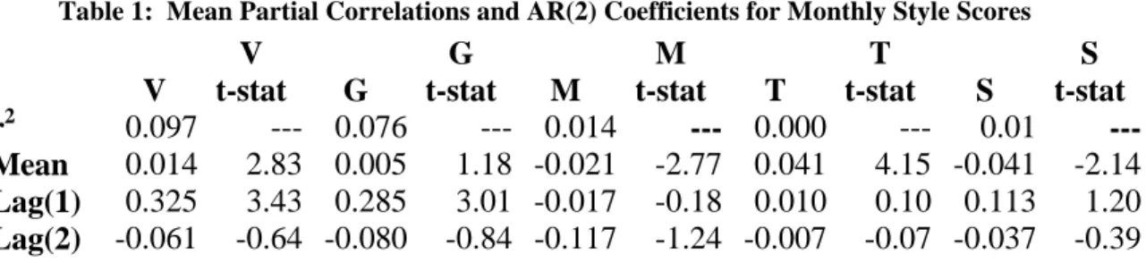
Table 1 shows the results of the coefficient autoregression analysis. Of the 15 coefficients that define the five return models, six are statistically significant when averaged over the sample time period. None of the second lags are significant, which

Timeliness 0 1 2 3 4 5 1 2 3 4 5 6 7 8 9 10 Safety 0 1 2 3 4 5 1 2 3 4 5 6 7 8 9 10

means that an AR(1) model should be sufficient. The significant variables are discussed below. Table 1 shows the coefficients for the Linear Model. It should be noted that the r-squared values represent the explained portion of the time series process of the style score concerned, not the explanatory power of that style score over the security returns.

Table 1: Mean Partial Correlations and AR(2) Coefficients for Monthly Style Scores

V V t-stat G G t-stat M M t-stat T T t-stat S S t-stat r2 0.097 --- 0.076 --- 0.014 --- 0.000 --- 0.01 ---Mean 0.014 2.83 0.005 1.18 -0.021 -2.77 0.041 4.15 -0.041 -2.14 Lag(1) 0.325 3.43 0.285 3.01 -0.017 -0.18 0.010 0.10 0.113 1.20 Lag(2) -0.061 -0.64 -0.080 -0.84 -0.117 -1.24 -0.007 -0.07 -0.037 -0.39

For the Value style score both the mean and lag(1) coefficients are both statistically significant. This means that, over the time period, there was a positive return to value, and that this return is positively autocorrelated – if the return to value is positive in one month, it will likely be positive the next month as well.

The Growth style score mean coefficient is not statistically significant, but the lag(1) coefficient is. This means that, over the time period, there is no consistent positive or negative return to growth, but the return is positively autocorrelated – if the return to growth is positive in one month, it will likely be positive the next month as well.

The correlation between the Momentum style score and return is strongly for positive, but the Lag 1 term is not. Figure 3 shows that only the lowest decile (the decile with the least momentum, which implies the highest negative momentum) has a positive relative return to the other deciles. This implies that the stocks that have performed the worst in the recent past will perform a little better in the next month.

The mean for Timeliness is positive, and with a very high average monthly t-statistic. This means that there has been a high and consistent return to timeliness over this period. The lag1 is very small; indicating the return to this factor is oscillating randomly about its mean.

The Safety First style score has a negative coefficient, indicating that high beta stocks have a higher realized return in this sample. This is consistent with CAPM. Figure 5 shows that there is a particularly high return to the highest beta (least safe) decile. The lag1 is moderately high, indicating a slight positive autocorrelation pattern to this factor.

We now turn to the key question of this research. In order to determine if there are

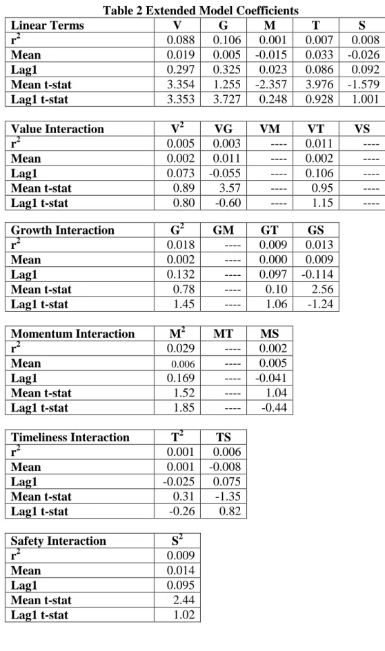
nonlinear (higher order or factor interaction) terms have any impact on returns, we extend our model by adding the squared terms and all combinations of interaction terms. We repeat the estimation of the linear model, while reducing the autoregressive estimation to a lag of one. The results are shown in Table 2.

Table 2 Extended Model Coefficients Linear Terms V G M T S r2 0.088 0.106 0.001 0.007 0.008 Mean 0.019 0.005 -0.015 0.033 -0.026 Lag1 0.297 0.325 0.023 0.086 0.092 Mean t-stat 3.354 1.255 -2.357 3.976 -1.579 Lag1 t-stat 3.353 3.727 0.248 0.928 1.001 Value Interaction V2 VG VM VT VS r2 0.005 0.003 ---- 0.011 ---- Mean 0.002 0.011 ---- 0.002 ---- Lag1 0.073 -0.055 ---- 0.106 ---- Mean t-stat 0.89 3.57 ---- 0.95 ---- Lag1 t-stat 0.80 -0.60 ---- 1.15 ---- Growth Interaction G2 GM GT GS r2 0.018 ---- 0.009 0.013 Mean 0.002 ---- 0.000 0.009 Lag1 0.132 ---- 0.097 -0.114 Mean t-stat 0.78 ---- 0.10 2.56 Lag1 t-stat 1.45 ---- 1.06 -1.24 Momentum Interaction M2 MT MS r2 0.029 ---- 0.002 Mean 0.006 ---- 0.005 Lag1 0.169 ---- -0.041 Mean t-stat 1.52 ---- 1.04 Lag1 t-stat 1.85 ---- -0.44 Timeliness Interaction T2 TS r2 0.001 0.006 Mean 0.001 -0.008 Lag1 -0.025 0.075 Mean t-stat 0.31 -1.35 Lag1 t-stat -0.26 0.82 Safety Interaction S2 r2 0.009 Mean 0.014 Lag1 0.095 Mean t-stat 2.44 Lag1 t-stat 1.02

The extended model first order coefficients and t-statistics changed very little from the linear model. The only higher order terms that are statistically significant at the 95% level are the VG interaction term and the S2 term. TheVG interaction term may

represent an additional return for stocks for which both value and growth are high. The S2 represents the additional return seen in the lowest deciles of Figure 5.

There are, however, a number of terms that are significant at the 90% level when

averaged over the period, including: the lag for the G2 term, the mean and lag for the M2 term, and the mean for the TS interaction term. We have been able to establish that a few of the higher order terms appear significant when averaged over the entire period and there may be some autoregressive properties to the time-series behavior of the

coefficients. It appears that asset-pricing models based on equity style factors ought give at least some meaningful consideration to the issues of second order and interaction terms.

Let us now turn our attention to the question of whether second order and interaction effects are important to the variation in securities return from period to period, the estimation of covariance between stocks and hence the issue of portfolio risk. It is entirely possible that a style score is highly significant with positive sign in one period and highly significant with a negative sign in the subsequent period. Even if not significant on average over the two periods, the strong effect in each period would be of the utmost importance to investors trying to forecast portfolio risk.

To do this, we’ll examine the absolute value of the t-statistics on our cross-sectional correlation coefficients. Given the sample period of one hundred twenty six months, we would expect that even random process would generate some coefficients that appeared statistically significant among the many trials. If the number of periods where the absolute value of the t-statistics is high is much greater than would be expected under a random process, we can conclude that this style score is meaningful from a risk

Table 3: Frequency of Months with t-Statistics with Absolute Value > 2

Value 40

Growth 32

Momentum 39

Timeliness 61

Safety First 85

Value

40

Growth

₁₆

Momentum

₄₃

Timeliness

₃₅

Safety First

₄₃

Value

××××

Growth

18

Value

××××

Timeliness

11

Growth

××××

Timeliness

12

Growth

××××

Safety First

15

Momentum

××××

Safety First 32

Timeliness

××××

Safety First

36

Of the twenty terms in the extended model (5 linear, 5 second order and 10 interaction), fifteen have frequencies of high absolute value t-statistics that are far above what would be expected merely coincidental relationships. All of both the linear and second order terms were persistently important.

Among the linear terms, the most noteworthy item would be that the “Safety First” style score had a significant t-statistic in approximately two thirds of the monthly sample periods. This provides a strong argument that conventional risk measures such as market beta and past total volatility are indeed efficient estimators of future risks. The

“Timeliness” measure also was frequently significant. When considered with the significant time series positive mean for “Timeliness”, we can see that the Timeliness model of Apt and Godfredsen appears to successfully predict future stock returns on a consistent basis.

For the second order terms, the frequency of high absolute value t-statistics was approximately half that for the comparable linear term, with the exception of the

“Momentum” style score. For Momentum, the second order term was important in more monthly periods than its linear cohort.

Among the ten interaction terms, five had frequencies of high absolute value t-statistics that were well in excess of random expectations. Of these, by far the strongest effects were seen in the interaction of the “Safety First” style score with “Momentum” and “Timeliness”

Conclusions

Investment style, as described the Northfield style scores, is meaningfully related to stock returns through both linear and nonlinear relationships. At least one defined investment style, “Timeliness” appears to successfully predict stock returns in conflict with the

efficient market assumptions of linear asset pricing models. We also confirm the earlier findings of diBartolomeo as to existence of strong time series properties in the returns to the style scores.

The “Momentum” style score shows clear evidence of a significant second order effect. This is immediately apparent upon visual inspect of the decile analysis. The

cross-sectional regressions confirm the strong non-linear nature of this effect. This information may be an important clue to a long running debate among practitioners as to the relative merits of value and momentum strategies. To the extent that the simplest value strategies may just be negative momentum strategies, it would appear that portfolios tilted toward either strong positive momentum or strong negative momentum would outperform a momentum neutral portfolio. Both sides of the argument may be right.

Our investigation of second order and interaction effects suggest that these effects are more strongly felt in forecasting of portfolio risk rather than return expectations. Nonlinear style effects are persistently important in understanding the variation in stock returns from period to period.

There is an important implication for practitioners. Both passive and active managers are generally interested in controlling the active return risk (tracking errors) of their

portfolios, relative to benchmark market indices. Our results suggest that merely

matching the average style attributes of their portfolio to their benchmark is insufficient. Successful risk control requires that the distribution of style attribute for a portfolio match the distribution of the same style attribute for the benchmark.

References

Abhyankar, Copeland and Wong. “Nonlinear Dynamics in Real Time Equity Market Indices: Evidence from the United Kingdom,” Economics Journal, 1995.

Aggrawal, Pankaj, Don Johnson and Donald Waggle, “Interaction Between Value Line’s Timeliness and Safety Ranks,” Journal of Investing, 2001.

Apt, Adam, Dan diBartolomeo and Eugene Godfredsen. “Trend Extrapolation Strategies for the US Stock Market,” Northfield Annual Conference Proceedings, Key West, 1993.

Arnott, Robert , John Dorian and Rosemary Macedo. “Style Management: The Missing Element in Equity Portfolios,” Journal of Investing, 1992.

Arshanapalli, Bala, T.Daniel Coggin, John Doukas and H. David Shea. “The Dimensions of International Equity Style,” Journal of Investing, 1998.

Christopherson, Jon. “Equity Style Classifications,” Journal of Portfolio Management, 1995.

diBartolomeo, Dan. “Time Series Properties of Valuation Models,” Northfield Working Paper, Boston, 1996

Elton, Edwin and Martin Gruber. “Portfolio Analysis with a Nonnormal Multi-Index Return Generating Model,” Review of Quantitative Finance and Accounting, 1992. Estep, Tony. “Manager Style and the Source of Equity Returns,” Journal of Portfolio Management, 1987.

Farrell, James. The Multi-Index Model and Practical Portfolio Analysis, The Financial Analysts Research Foundation Occasional Paper No. 4, 1976.

Fama, Eugene F. and James D. MacBeth. “Risk, Return and Equilibrium: Empirical Tests,” Journal of Political Economy, 1973.

Fama, Eugene F. and Kenneth R. French. “The Cross-Section of Expected Stock Returns,” Journal of Finance, 1992

Gallo, John and Larry Lockwood. “Benefits of Proper Style Classification of Equity Portfolio Managers,” Journal of Portfolio Management, 1997.

Grinold, Richard. “Is Beta Dead Again?,” Financial Analyst Journal, 1993 Guy, James and Barr Rosenberg. “Beta and Investment Fundamentals,” Financial Analyst Journal, 1976.

Lakonishok, Josef, Andrei Schliefer and Robert Vishny. “Contrarian Strategies, Extrapolation and Risk,” Journal of Finance, 1994

Lebaron, Blake and Jose Scheinkman. “Nonlinear Dynamics and Stock Returns,” Journal of Business, 1989.

Michaud, Richard. “Is Value Multidimensional? “Implications for Style Management and Global Stock Selection,” Journal of Investing, 1998.

Qi, Min. “Nonlinear Predictability of Stock Returns Using Financial and Economic Variables,” Journal of Business and Economic Statistics, 1999.

Quinton, Keith. “Consensus Growth Estimates and Stock Selection,” Northfield Annual Conference Proceedings, Key West, 2000

Reinganum, Marc. “Misspecification of Capital Asset Pricing: Empirical Anomalies Based on Earnings Yield and Market Values,” Journal of Financial Economics, 1981. Rosenberg, Barr. “Extra-Market Components of Covariance in Security Returns,”

Journal of Financial and Quantitative Analysis, 1974.

Ross, Stephen. “An Arbitrage Theory of Capital Asset Pricing,” Journal of Economic Theory, 1976.

Sharpe, William. “Capital Asset Prices: A Theory of Market Equilibrium under Conditions of Risk,” Journal of Finance, 1964.

Willey, Thomas. “Testing for Nonlinear Dependence in Daily Stock Indices,” Journal of Economics and Business, 1992.

Appendix

The five styles that were modeled are:

Value Growth

Price Momentum

Sector Rotation (also referred to as Timeliness) Safety First

At each month-end since April of 1991, each stock in the Northfield universe was given a score of 0 to 100 for each of the five listed models. The scores are normalized percentile ranks. Each of the five models is a composite of two to eight sub-models. Each model ranking is an equal-weighted combination of the rankings of the sub-models included within that model.

It should be noted that the process of surveying managers and tabulating those surveys was done without any regard to the past performance or business success of the

managers. As such, there is no a priori reason to believe that these models would lead to a ranking system that would produce superior investment results. Rather, the rankings portray the level of probable attractiveness that a given stock would have for each type of manager at a particular moment.

The "Value" model has five components (sub-models). These are:

a) Dividend Discount Model b) Graham-Dodd Formula

c) Relative Value to Universe (cross-sectional regression of P/E, P/B, and Yield) d) Relative Value Within Industry (cross-sectional regression of P/E, P/B and Yield) e) Time Series of Price/Value Ratio, with Value defined as 12 month EPS

capitalized at the T-Bill rate

The “Growth” model has eight components. These are:

a) True Growth rate as defined by EUPS (an elaborate model of corporate growth and reinvestment)

b) True Growth Consistency as defined by EUPS

c) Earnings Momentum (2nd derivative with respect to time of a curve fit to the EPS time series)

e) Estimate Revision 1 Month ((no. of up revisions - number of down revisions) / (no. of analysts))

f) 5-Year Trend of Sales and 5-Year Trend of Margins g) 5-Year Growth of Dividends

h) “Torpedo Effect" (assumes stocks with highest earnings-growth expectations will disappoint)

The "Price Momentum" model has four sub models. These are:

a) 52 Week Jensen's Alpha b) 52 Week Relative Strength

c) Consistency of 5-year price increases

d) Asymmetry of Regression beta (up markets minus down markets)

The "Sector Rotation" (Timeliness) model has two sub-models: These are:

a) Expected Jensen's alpha based on Factor Exposure b) Expected Jensen's alpha based on Industry Participation

Details of the construction of the Timeliness model and its two sub-components can be found in Trend Extrapolation Strategies by Adam J. Apt, Ph.D. and Eugene A.

Godfredsen, Ph.D., Northfield Conference Proceedings, 1993. The model starts with standard CAPM assumptions. Each month a cross-sectional regression analysis is performed, which yields the statistical relationship between observed Jensen's alpha (at the individual security level) and sixty-six fundamental characteristics of stocks (11 continuous variables such as P/E, Yield, Size, etc. and 55 "dummies" for industry groups). As this process is repeated each month, a time series is created for each of the sixty-six factors. Using the time series methods of Box and Jenkins, an ARIMA (1,0,1) model is used to forecast the expected next value in each of the sixty-six series. Given these forecasts of factor alpha, a forecast of alpha for each stock is calculated as the vector product of the observed factor exposures times the expected factor alphas.

The "Safety" model has two components. These are:

a) Forecast Beta. Historical regression beta adjusted to reflect changes in company fundamentals

b) Price Volatility, calculated as (52-week high - 52-week low) / (52-week high + 52-week low)