Image recognition with Deep Learning techniques and TensorFlow

(1)

Universitat Politècnica de Catalunya (UPC) - BarcelonaTech

Facultat d’Informàtica de Barcelona (FIB)

Image Recognition with Deep Learning

Techniques and TensorFlow

Maurici Yagües Gomà

Master in Innovation and Research in Informatics

Data Mining and Business Intelligence

Advisor

: Jordi Torres Viñals

Universitat Politècnica de Catalunya (UPC) Department of Computer Architecture (DAC)

Co-Advisor

: Ruben Tous Liesa

Universitat Politècnica de Catalunya (UPC) Department of Computer Architecture (DAC)

(2)

Abstract

Deep neural networks have gained popularity in recent years, obtaining outstanding results in a wide range of application, but most notoriously in computer vision and natural language processing tasks. Despite the newly found interest, research in neural networks span many decades back, and some of today’s most used network architectures where invented many years ago. Nevertheless, the progress made during this period cannot be understood without taking into account the technological advancements seen in key contiguous domains such as massive data storage and computing systems, more specifically in the Graphic Processing Unit (GPU) domain. These two components are responsible for the enormous performance gains in neural networks, that have made what we call Deep Learning a common word among the Artificial Intelligence and Machine Learning community.

These kind of networks need massive amounts of data to effectively train the millions of parameters they contain, and this training can take up to days or weeks depending on the computer architecture we are using. The size of new published datasets keeps growing, and the tendency of creating deeper networks that outperforms shallower architectures means that on the medium and long term the computer hardware to undertake these kind of training processes can only be found in high performance computing facilities, where they have enormous clusters of computers. However, using these machines is not straightforward, as both the framework and the code need to be appropriately tuned for effectively taking advantage of these distributed environments.

For this reason, we test TensorFlow, an open-sourced framework for Deep Learning from Google that has built-in distributed support, on top of the GPU cluster, called MinoTauro, at Barcelona Supercomputing Center (BSC). We aim to implement a defined workload using the distributed features the framework offers, to speed up the training process, acquire knowledge of the inner workings of the framework and understand the similarities and differences with respect to a classic single node training.

(3)

(4)

Acknowledgements

I would like to express my gratitude to my advisor, Jordi Torres, for introducing me to the Deep Learning universe, his endless enthusiasm and guiding me through the making of this thesis. Also, to my co-advisor, Ruben Tous, for the wise comments and encouragement. To the Barcelona Supercomputing Center for the opportunity and to their Support Team for the prompt answers whenever a problem occurred.

To my colleagues at the Autonomic Systems and e-Business Platforms group, for the inter-esting talks at lunch and their constant support whenever there is a problem. Special thanks to Francesc Sastre, without whom this thesis will not have been finished on time.

Also, to all people I have met during these years at the master, for introducing me to new areas of informatics I did not know.

Thanks to my family and friends, for supporting me and being always there, in the good, the not so good, and the funny times.

(5)

(6)

1. Problem statement

1.1

Goals of this thesis

The aim of this master thesis is to test the scalability of the TensorFlow framework in the MinoTauro machine (GPU cluster) at Barcelona Supercomputing Center (BSC). This frame-work is oriented, but not constrained, to develop Deep Learning applications, and has built-in distributed computing for using multiple nodes of both CPUs and GPUs. A series of machine configurations will be tested with a defined workload, in order to understand the behaviour of both the framework and the machines.

Distributed training in deep learning is quite a recent tendency given the massive sizes of datasets coupled with the always increasing depth of the neural networks. As of today, mainly the big software companies use these systems internally for their own products, but out of the box versions were difficult to implement or were non-existent. TensorFlow is in ongoing development, and the amount of documentation for their distributed version is scarce, given that it is not the most used functionality, as not many users have access to clusters of GPUs.

1.2

Introduction to distributed machine learning systems

During the last decade machine learning has seen an increased interest from many different areas, becoming a key element in multiple industries. Although many of today’s algorithms rely on decades, or even centuries, old mathematics, their increased performance is a conse-quence of both more complex models and bigger volumes of data. The need for storing these large amounts of data (both structured and unstructured) has encouraged the research in new database formats, circumventing the constraints of old systems. The rise of distributed storage systems led to the need of machine learning algorithms that could benefit from that type of architecture, and that could cope with more complex models, even though that meant designing new algorithms or adapting old ones.

Part of this section takes the main ideas of the great introduction in Bekkerman, Bilenko, and Langford [5], presenting some general concepts of applying machine learning in distributed environments. Furthermore, an overview of deep learning and the current state of distributed machine learning is presented.

1.2.1

Scaling up machine learning

Distributed computing has emerged as an efficient solution for tackling growing machine learning challenges. These platforms allow the scalability of machine learning tasks, enabling

(9)

some properties that could not be achieved with single-machine processing:

• Larger number of data instances: combining the distributed storage and bandwidth of a cluster of machines the amount of data that can be processed is increased.

• Higher input dimensionality: some tasks involving natural language, video or biolog-ical data are prone to a high number of features. Parallelizing the computation across features can be used for scaling up the process.

• Model and algorithm complexity: running complex non-linear models that are com-putationally expensive can be alleviated with distributed computing by means of parallel multicore or multinode, and the use of coprocessors such as GPUs.

• Model selection and parameter tuning: for these kind of tasks parallelization is straightforward as they consist of independent executions of the same dataset, with dif-ferent combinations of hyper-parameters.

However, scaling up the computation to a distributed system is also a more difficult task than working on a single machine. Depending on the efficiency of the algorithm, communication between nodes can be a bottleneck, and the system has to be robust in order to overcome possible failures.

1.2.2

Types of parallelism

The main idea behind this computing paradigm is to run tasks concurrently instead of serially, as it would happen in a single machine. To achieve this, there are two principal implementations, and it will depend on the needs of the application to know which one will perform better, or even if a mix of both approaches can increase the performance.

Data parallelism

In this mode, the training data is divided into multiple subsets, and each one of them is run on the same replicated model in a different node (worker nodes). These will need to synchronize the model parameters (or its gradients) at the end of the batch computation to ensure they are training a consistent model. This is straightforward for machine learning applications that use input data as a batch, and the dataset can be partitioned both rowwise (instances) and columnwise (features).

Some interesting properties of this setting is that it will scale with the amount of data available and it speeds up the rate at which the entire dataset contributes to the optimization [51]. Also, it requires less communication between nodes, as it benefits from high amount of computations per weight [38]. On the other hand, the model has to entirely fit on each node [15], and it is mainly used for speeding computation of convolutional neural networks with large datasets.

Model parallelism

In this case, the model will be segmented into different parts that can run concurrently, and each one will run on the same data in different nodes. The scalability of this method depends on the degree of task parallelization of the algorithm, and it is more complex to implement than the previous one. It may decrease the communication needs, as workers need only to synchronize

(10)

the shared parameters (usually once for each forward or backward-propagation step) and works well for GPUs in a single server that share a high speed bus [14]. It can be used with larger models as hardware constraints per node are no more a limitation, but is highly vulnerable to worker failures.

1.2.3

Performance metrics

The term performance in these systems has a double interpretation. On one hand it refers to the predictive accuracy of the model, and on the other to the computational speed of the process. The first metric is independent of the platform and is the performance metric to compare multiple models, whereas the second depends on the platform on which the model is deployed and is mainly measured by metrics such as:

• Speedup: ratio of solution time for the sequential algorithms versus its parallel counter-part

• Efficiency: ratio of speedup to the number of processors

• Scalability: efficiency as a function of an increasing number of processors

Some of this metrics will be highly dependent on the cluster configuration, the type of network used and the efficiency of the framework using the libraries and managing resources.

1.3

Deep learning overview

Despite having gained a lot of notoriety in the last years, research in multilayer neural networks span many decades [57]. Conventional machine learning techniques had difficulty in processing natural data in their raw form, so to make classifiers more powerful it was common to use generic non-linear features such as kernel methods and create multi-stage hand-tuned pipelines of extracted features and discriminative classifiers [55]. However, those generic features did not allow the learner to generalize well from the training examples, so one of the main advantages of these new methods is the fact that good features can be learned automatically using a general purpose learning procedure and without human engineering [41]. That is why deep learning techniques are also referenced as representation learning methods that are fed with raw data and have multiple levels of representation, obtained by composing simple but nonlinear modules that each transform the representation at one level into a representation at a higher, slightly more abstract level [41, 7]. These methods have dramatically improved the state of the art in recent years in multiple areas such as speech recognition, visual object recognition and detection, drug discovery and genomics.

1.3.1

Early tendencies and evolution

Early works of multilayer neural networks date back to Ivakhnenko [34] for Feedforward Multilayer Perceptron type networks and to Fukushima [20] for today’s version of convolutional neural networks, inspired by the structure of the nervous visual system, having lower order hypercomplex cells in the early layers and higher order hypercomplex cells in the latest ones. Although this works mainly established the structure for deep neural networks that was later popularised, they still lacked a good learning algorithm for weight updates during the training phase. It was not until the mid 80s that backpropagation was popularised for neural networks

(11)

by Rumelhart, Hinton, and Williams [54]. With backpropagation the error values at the output are back propagated using the chain rule to compute the gradient of the error with respect to each weight [26]. This way the weights get updated at each step with the objective to minimize a loss function. LeCun et al. [42] were the first to apply backpropagation to the network architecture presented by Fukushima [20] to recognize handwritten zip code digits (MNIST dataset). Backpropagation is still today the dominant approach for training deep networks.

However, backpropagation for feedforward neural networks and recurrent neural networks seemed to work only for shallow structures and suffered from the vanishing or exploding gra-dient problem. That means cumulative backpropagated error signals either shrink rapidly, or grow out of bounds, making deep structures impossible to train [57]. This led to the Long Short-Term Memory (LSTM) cell [31] that outperformed the performance of recurrent neural networks on tasks that require learning the rules of regular languages, and tasks involving con-text free languages that could not be represented by Hidden Markov Models. In addition, this new method did not suffer from the vanishing or exploding gradients. In recent years these kind of structures have improved the state of the art in applications such as protein analy-sis, handwriting recognition, voice activity detection, optical character recognition, language identification, audio onset detection, text-to-speech synthesis, social signal classification and machine translation [57].

All in all, ventures based on neural networks and other AI technologies began to make un-realistically ambitious claims while seeking investments. When AI research did not fulfill these unreasonable expectations, investors were disappointed, which led to a decline of popularity of neural networks until the mid 2000s [24]. That gap was filled with other methods such as Support Vector Machines, kernel methods and graphical models that dominated many practical and commercial pattern recognition applications during that time [57].

The expression Deep Learning was coined around 2006 with the publication of structures such as a stack of Restricted Boltzmann Machines called Deep Belief Network that arouse inter-est for the good results obtained [30]. At the same time, early tests on GPU-based convolutional neural networks made training times several times faster, and by 2010 a GPU implementation of backpropagation was up to 50 times faster than its CPU version [57].

1.3.2

Recent years

Certainly advancements in computer hardware are of main importance in developing deeper architectures that can build more complex models. Neural networks have doubled in size roughly every 2.4 years with the availability of faster CPUs at first and the advent of general purpose GPUs later, in addition to better software infrastructure for distributed computing [24]. Also, the digitization of society has made possible the availability of gigantic datasets that can be used to successfully train neural networks. ImageNet is an image database with 1.2 million images with 1000 different categories organized according to the WordNet hierar-chy and has, at least, 732 images per class, making it one of the biggest datasets available. Different tracks are available, image classification, single and multiple-object localization, or object detection in videos, with classifications for models using the provided data and another for those that use additional resources. Since 2012, deep convolutional networks have won the ImageNet competition for object classification, and by 2014 all top contestants were relying on convolutional neural networks [55].

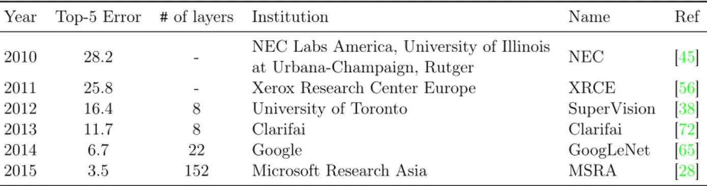
Table 1.1 and Table 1.2 show the progress convolutional neural networks have achieved in image classification and single-object localization, challenges started at 2010 and 2011,

(12)

respec-tively. For those years, the winners used methods related to support vector machines, but since then increasingly deeper neural networks have been topping the results, with notable gains year after year.

Table 1.1: Summary of winning teams in the ImageNet image classification challenge. (Source: Russakovsky et al. [55] with some additions)

Year Top-5 Error #of layers Institution Name Ref

2010 28.2 - NEC Labs America, University of Illinois

at Urbana-Champaign, Rutger NEC [45]

2011 25.8 - Xerox Research Center Europe XRCE [56]

2012 16.4 8 University of Toronto SuperVision [38]

2013 11.7 8 Clarifai Clarifai [72]

2014 6.7 22 Google GoogLeNet [65]

2015 3.5 152 Microsoft Research Asia MSRA [28]

Table 1.2: Summary of winning teams in the ImageNet single-object localization. (Source: Russakovsky et al. [55] with some additions)

Year Error Institution Name Ref

2011 42.5 University of Amsterdam, University of Trento UvA [70] 2012 34.2 University of Toronto SuperVision [38]

2013 30.0 New York University OverFeat [58]

2014 25.3 University of Oxford VGG [61]

2015 9.0 Microsoft Research Asia MSRA [28]

1.3.3

Current uses and tendencies

The domain of application and research of deep learning techniques has progressed a lot in a small span of time. Image classification was the first application where deep neural net-works began showing incredible results. The ImageNet challenge pushed the research of many groups in this area, with incredible results, as seen in the previous section, in the domains of image classification, single and multiple-object localization, and object detection in videos as of recently.

However, convolutional neural networks have been used in some varied applications such as in Gatys, Ecker, and Bethge [22], where these kind of networks are able to modify the content of a photo to match the style of a picture. Using the pre-trained network in Simonyan and Zisserman [61] the new image is approximated to both, the activations at some layer of the original content, and the Gram matrix of the activations of the style image. The user can tune the weight of the content and the style in the final picture adjusting some hyperparameters in the loss function, and choose the layers to take into account in the optimization process. This approach was later applied to video by Ruder, Dosovitskiy, and Brox [53] and Anderson et al. [4], and some alternative implementations of the original neural art appeared during the last year [11,21, 35, 48, 69].

Other neural network architectures have also benefited from deeper models, more compu-tational power and bigger datasets. Recurrent neural networks and LSTM have been used for some years related to natural language processing fields, improving the state of the art in

(13)

(a)City of London skyline (Photo by DAVID ILIFF)1 _(b) _{Style from Vincent van Gogh’s}_{The Starry Night}

Figure 1.1: Example of neural art with own implementation.

applications such as language translation [13, 64], speech-to-text recognition [25] and senti-ment analysis [63]. Vinyals et al. [71] coupled the powerful architecture of convolutional neural networks for image recognition to a recurrent neural networks, to create a generative model that can output a description of an image given as input. Recently, a group of people from the Google Brain has been developing algorithms for music generation with recurrent neural networks [52].

Another successful application that had a lot of attention in the media was the win of the Google DeepMind project AlphaGo2 to Go professional player Lee Sedol. Go had been till then a much more difficult feat for artificial intelligence, due to its enormous search space and the difficulty of evaluating board position and moves. Prior to this match, the program was paired to another Go player, Fan Hui, and the details of the match can be found at Silver et al. [60]. The paper also explains the methods used for building AlphaGo, which uses: convolutional networks for creating a representation of the position, supervised learning for training a policy network from human expert moves, reinforcement learning for optimizing the policy network in games of self-play, value networks for evaluating the board positions and predicting the winner of the game, and paired with the Monte Carlo tree search that estimates the value of each state in the tree of all possible sequence of moves.

Given the costs of computation of the networks, they used asynchronous multi-threaded searches, executing simulations on CPUs, and computing policy and value networks in parallel on GPUs. The final version of AlphaGo used 40 search threads, 48 CPUs, and 8 GPUs, but a distributed version was tested with 40 search threads, 1,202 CPUs and 176 GPUs. Their version was tested against other programs available, winning most of the matches even when free moves where allowed for the opponents. During the match against Lee Sedol a custom ASIC, called TPU was used [16,36], which is more energy efficient than GPUs, and is specially tailored for machine learning tasks, as it is optimized for low precision computations that have proved to work well in inference.

1_{License: CC-BY-SA 3.0 (}_Wikipedia₎ 2_{AlphaGo webpage}

(14)

1.3.4

Framework comparison

Given the amount of interest in these algorithms, many frameworks specialized in this area have appeared in the last years3_{. However, most of them where designed for efficient single-node} computation with multiple devices (CPUs and GPUs), and their distributed applications were dependent on other frameworks of distributed processing (Spark, Hadoop, etc.).

The appearance of new programming models, such as MapReduce [17], that built on old approaches like Message Passing Interface, has shifted the computation of many companies to distributed configurations. This new models make it easy to parallelize tasks on many servers, taking advantage of the distributed storage system for efficient computation. However, state-of-the-art deep learning systems rely on custom implementations to facilitate their asynchronous, communication-intensive workloads [47]. As a consequence, some deep learning frameworks with only single-node computing capabilities have been used on top of those parallelizing sys-tems to obtain a satisfactory degree of performance.

With the growing expansion of deep learning, some frameworks with different properties and options have been appearing during the last years. Table 1.3 resumes some properties of a reduced selection of frameworks available for deep learning.

Table 1.3: Framework comparison. (Source: Tokui et al. [68] with some additions)

Caffe CNTK MXNet TensorFlow Theano Torch

Started

from* 2013 2014

4 ₂₀₁₅ ₂₀₁₅ ₂₀₀₈ ₂₀₁₂

Main

developers BVLC

5 _Microsoft _DMLC6 _Google Université

de Montréal

Facebook, Twitter, etc.7 Core

languages C++ C++ C++ C++, Python C, Python C, Lua

Supported languages

C++, Python

MATLAB CLI

C++, Python

R, Julia, Go... C++, Python C, Python C, Lua Parallel

computation Multi GPU

Multi GPU Multi-node

Multi GPU

Multi-node8 Multi GPU Multi GPU *Year of GitHub repository creation

Most of the broadly used frameworks enable multi-device computation and support both CPUs and GPUs. Also, most of them enable by now parallel computing in single node envi-ronments (multi GPUs), and some of the newest begin supporting multi-node architectures, although this is a much more scarce feature, given the complexity of the implementation and that not many users have access to clusters of GPUs.

Performance on single-node execution is similar across frameworks, as they rely on similar implementations for running on GPUs [1]. Differences may arise in the way each framework handles memory allocation or other specific design choices of the developers. As Adolf et al. [3] summarize, there is a convergent evolution amongst the more popular libraries. For example,

3_{At least 40 according to the following list (}_{Deep Learning Software links}₎ 4_{Released on January 2016 (}_announcment₎

5_{Berkeley Vision and Learning Center (}_BVLC₎

6_{Distributed (Deep) Machine Learning Community (}_dmlc.ml₎

7_{Ronan Collobert, Clement Farabet, Koray Kavukcuoglu, Soumith Chintala (}_{list of contributors}₎ 8_{Since version 0.8.0 RC0 in April 2016 (}_{release notes}₎

(15)

they all use a simple front-end specification language, optimized for productivity, and highly-tuned native backend libraries for the actual computation.

As said before, prior to the appearance of native distributed versions, some experiments were done combining single-node frameworks with parallel engines. For instance, Caffe is a framework that can be used on multiple GPUs in a single-node machine, and has been applied to a distributed environment with SparkNet [47] and CaffeOnSpark [19], developed by the Yahoo Big ML Team. Prior to open sourcing the native distributed implementation of TensorFlow, its single-node version was scaled with Spark by Databricks [32], for hyperparameter tuning, and Arimo [62], for scalability tests.

Other trends include the addition of extensions and libraries to those frameworks that enable multi-node capabilities without the need of a middle layer as Spark. Theano-MPI is a framework, built on Theano, that supports both synchronous and asynchronous training of models in data parallelism setting on multiple nodes of GPUs [46]. In the case of Caffe, FireCaffe offers similar properties for scaling the training of complex models [33], and for Torch, the Twitter Cortex team developed a distributed version [66].

1.4

Framework used: TensorFlow

TensorFlow9 was open-sourced on November 2015, as a software library for numerical com-putation using data flow graphs [2]. Despite its extended library for deep learning functions, the system is general enough to be used for many other domains. This system is the evolution of the previous scalable framework DistBelief, supports large-scale training and inference in multiple platforms and architectures, and aims to be a flexible framework for both experiment-ing and runnexperiment-ing in production environments. This is achieved by usexperiment-ing dataflow programmexperiment-ing models (Spark, MapReduce) which provide a number of useful abstractions that insulate from low-level details of distributed processing. Then, communication between subcomputations is explicit and makes it easy to partition and run independent sub-graphs on multiple distributed devices.

The node placement algorithm uses a greedy heuristic for examining the completion time of every node on each possible device, including communication costs across devices. The graph is then partitioned into a set of subgraphs, one per device, andReceive andSend nodes are added to the incoming and outgoing connections, as Figure 1.2a shows. These will coordinate the transfer data across devices, making the scheduling of the nodes decentralized into the workers. The native distributed version of TensorFlow builds up from DistBelief, which could utilize computing clusters with thousands of machines [18]. The parameter server architecture pre-sented in Li et al. [43] manages asynchronous data communication between nodes, and supports flexible consistency models, elastic scalability, and continuous fault tolerance. This architecture uses a set of servers to manage shared state variables that are updated by a set of data-parallel workers. In essence, variables of the model are stored in the parameter servers, and are loaded to each worker for the computation, with the batch of data. The workers return the gradients obtained to the parameter servers, where the variables are updated and sent again for the next computation (Figure 1.2b).

Initial implementations of the parameter server were (key, value) pairs, where for LDA the pair is a combination of the word ID and the topic ID. The implementation in [43] treats these

(16)

(a) Placement of Send/Receive nodes.

(Source: Abadi et al. [2]) (b) Parameter server architecture. (Source: Dean et al. [18])

Figure 1.2: Architecture details of TensorFlow.

objects as sparse linear algebra objects, by assuming that keys are ordered, and those missing are treated as zeros, which enables optimized operations for vectors.

TensorFlow implements a user-level checkpointing for fault-tolerance, so that a trained model can be restored in the event of a failure. Those checkpoints need not to be consistent, unless strictly specified, and is a choice of the user to define the checkpoint retention scheme. This enables easy reutilization of models for fine-tuning or unsupervised pre-training [1].

Another interesting feature is the visualization tool named TensorBoard, that enables com-putation graph and summary data visualizations, for better understanding of the model defined and the training process. Some internal features made it possible to build a tracing profile of the model, so that the user can track the device placement of every node, node dependencies and computation time.

For this project, the version used is the latest stable one available 0.10.0, and all the scripts and models have been built with the Python API. Further details of the implementation will be specified when necesseary in the following sections.

1.4.1

Types of data parallelism

TensorFlow enables multiple strategies for aggregating the results in multinode settings when working with data parallelism. Chen et al. [12] compare different methods, with varying results in model accuracy and training speeds for up to 200 different nodes. The workers will have a similar task in both cases, but it is the way the model is updated at the parameter servers that makes the key difference between these two approaches.

(a) Asynchronous replication (b) Synchronous replication (c)Synchronous with backup workers Figure 1.3: Strategies for data parallelism. (Source: Abadi et al. [1])

(17)

Asynchronous mode

In this mode, each worker replica will be computed independently of the computations in other nodes, so no problems will arise if one of them crashes. They will follow these steps for every batch iteration:

1. The worker fetches from the parameter servers the most up-to-date model needed to process the current batch

2. Computes the gradients of the loss with respect to these parameters 3. Sends back the gradients to the parameter servers

The parameters servers will then update the model accordingly, and sent it to the worker for the next computation. The idea is the model on the parameter servers will be updated each time a worker sends the gradients (Figure 1.3a). This makes it easy to implement large scale training processes in architectures that may have different types of hardware, as each one will behave independently, and they maintain high throughput in the presence of stragglers.

The problem for this strategy is that individual steps use stale information, making each step less effective [1], so when a model is trained with N workers, each update will be N −1

steps old on average. It may happen that by increasing the number of workers, the training results worsen with the noise introduced by the discrepancy between the model used to compute gradients and the model that will be updated in the parameter server [12].

Synchronous mode

With this setting, the workers will behave as before, as they only need to make gradient computation, but the parameter servers will wait for all the workers to send the gradients before proceeding to the model update, using queues for accumulating and applying them atomically. It means that at the start of the batch iteration, each worker will have the most up-to-date model, and the gradients will be computed from the same parameter values (Figure 1.3b).

Given that, for this case, the model in each worker is the same, the batch contains different items and the gradient computation is done all at once, it can be seen as a single step with a batch size N times bigger. According to results in Chen et al. [12] synchronous training can achieve better accuracy, needs fewer epochs to converge and has less accuracy loss when increasing the number of workers. However, the update time of the model depends on the slowest worker, as the parameter servers need to wait until the end of the execution in every one of them, so time per batch may be slower than in the asynchronous case. In order to mitigate this effect, a possible workaround is to implementbackupworkers, so that the parameter servers update the model when they have collected the gradients from m of n workers (in Figure 1.3c

m= 2 and n= 3).

Despite the several publications from Google demonstrating the different results between synchronous and asynchronous modes [1,12], the public version of TensorFlow has not a working implementation for the synchronous training10 11 _{in multinode.}

10_{GitHub issue}_#3458 11_{Synchronous example (}_link₎

(18)

1.5

Platform

BSC-CNS (Barcelona Supercomputing Center – Centro Nacional de Supercomputación) is the National Supercomputing Facility in Spain and was officially constituted in April 2005. BSC-CNS manages MareNostrum, one of the most powerful supercomputers in Europe. The mission of BSC-CNS is to investigate, develop and manage information technology in order to facilitate scientific progress. With this aim, special dedication has been taken to areas such as Computer Sciences, Life Sciences, Earth Sciences and Computational Applications in Science and Engineering.

All these activities are complementary to each other and very tightly related. In this way, a multidisciplinary loop is set up: “our exposure to industrial and non-computer science academic practices improves our understanding of the needs and helps us focusing our basic research towards improving those practices. The result is very positive both for our research work as well as for improving the way we service our society” [9].

BSC-CNS also has other High Performance Computing (HPC) facilities, as the NVIDIA GPU Cluster MinoTauro that is the one used for this project.

1.5.1

MinoTauro overview

MinoTauro is a heterogeneous cluster with 2 configurations [10]:

• 61 Bull B505 blades, each blade with the following technical characteristics:

– 2 Intel E5649 (6-Core) processor at 2.53 GHz

– 2 M2090 NVIDIA GPU Cards

– 24 GB of main memory

– Peak Performance: 88.60 TFlops

– 250 GB SSD (Solid State Disk) as local storage

– 2 Infiniband QDR (40 Gbit each) to a non-blocking network

– 14 links of 10 GbitEth to connect to BSC GPFS Storage • 39 bullx R421-E4 servers, each server with:

– 2 Intel Xeon E5-2630 v3 (Haswell) 8-core processors, (each core at 2.4 GHz,and with 20MB L3 cache)

– 2 K80 NVIDIA GPU Cards

– 128 GB of Main memory, distributed in 8 DIMMs of 16 GB DDR4 @ 2133 MHz -ECC SDRAM

– Peak Performance: 250.94 TFlops

– 120 GB SSD (Solid State Disk) as local storage

– 1 PCIe 3.0 x8 8GT/s, Mellanox ConnectXR - 3FDR 56 Gbit

(19)

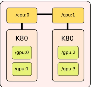
The operating system is RedHat Linux 6.7 for both configurations. The TensorFlow instal-lation is working only on the servers with the NVIDIA K80 because the M2090 NVIDIA GPU cards do not have the minimum required software specifications TensorFlow demands.

Each one of the NVIDIA K80s contain two K40 chips in a single PCB with 12 GB GDDR5, so we physically have only two GPUs in each server, but are seen as 4 different cards by the software.

K80

/gpu:0 /gpu:2 /gpu:3 /gpu:1 /cpu:1 /cpu:0

Figure 1.4: Schema of the hardware in a MinoTauro node

1.5.2

Software stack and queue system

MinoTauro uses the GPFS file system, which is shared with MareNostrum. Thanks to this, all nodes of MinoTauro have access to the same files. All the software is allocated in the GPFS system and is also common in all nodes, there are two software folders, the general folder and the K80 folder, the last folder contains all the software compiled for the NVIDIA K80 GPUs [10].

MinoTauro comes with a software stack, this software is static and the users can’t modify it. If a user needs a new software, a modification or an update of an existent software has to request a petition to the BSC-CNS support center. This is the used part of the software stack in this project:

• TensorFlow 0.812: The first version of TensorFlow used in this project. This version implements the distributed features and it was used on the first half of the project. • TensorFlow 0.1013_: _{The second release of TensorFlow used in this project. This version}

has a lot of bug fixes, improvements and new abstraction layer, TF-Slim, that allows to do some operations more easily.

• Python 3.5.2: The Python version installed in the K80 nodes. It comes with all required packages by TensorFlow.

12_{GitHub release}_0.8 13_{GitHub release}_0.10

(20)

• CUDA 7.5: CUDA is a parallel computing platform and programming model created by NVIDIA. It enables dramatic increases in computing performance by harnessing the power of the GPU [49]. This is required to use GPUs with TensorFlow.

• cuDNN 5.1.3: The NVIDIA CUDA Deep Neural Network library is a GPU-accelerated library of primitives for deep neural networks. cuDNN provides highly tuned imple-mentations for standard routines such as forward and backward convolution, pooling, normalization, and activation layers [50].

MinoTauro has a queue system to manage all the jobs sent by all users in the platform. To send a job to the system is necessary to do a job file with the job directives:

job_name The job’s name

initialdir Initial directory to run the scripts output The output file’s name

error The error file’s name

gpus_per_node Number of needed GPUs for each assigned node cpus_per_task Number of needed CPUs for each task

total_tasks Number of tasks to do wall_clock limit Maximum job time

features To request other features like K80 nodes

In order to obtain the maximum number of GPU cards, it is mandatory to set the parameter cpus_per_taskto 16, all cores in a node, and setgpus_per_nodeto 4. With this configuration the queue system will give a full node with 4 GPUs, two K80 cards, for each task. The fact that we ask for the maximum number of CPUs is for the system to assign different nodes, so we can effectively send the distributed jobs. Despite the fact that we are mainly interested in the computational capabilities of GPUs, powerful CPUs are needed in order to feed the GPUs as fast as possible, so as to not have any bottlenecks on the device.

This is an example of a job file: #!/bin/bash # @ job_name= job_tf # @ initialdir= . # @ output= tf_%j.out # @ error= tf_%j.err # @ total_tasks= 3 # @ gpus_per_node= 4 # @ cpus_per_task= 16 # @ wall_clock_limit = 00:15:00 # @ features = k80

module load K80 cuda/7.5 mkl/2017.0.098 CUDNN/5.1.3 python/3.5.2 python script_tf.py

This file defines a job with 15 minutes of maximum duration on 3 nodes with 4 GPUs on each. Once the job is submitted the queue system will give the job ID number to do tracking on the task:

Submitted batch job 87869

At the time that the queue system assigns the nodes for the task, the user can see which nodes have been assigned and connect to them to see their GPU an CPU usage among other

(21)

things. In the following job summary, we have been given all CPUs and GPUs in nodes 16, 19 and 25, during a maximum time of 15 minutes.

JOBID NAME USER STATE TIME TIME_LIMI CPUS NODES NODELIST(REASON) 87869 job_tf - RUNNING 0:02 15:00 48 3 nvb[16,19,25]

All the parameters and configurations for the MinoTauro queue system are available on the MinoTauro User’s Guide [10].

1.5.3

Distributed TensorFlow with Greasy

To run distributed TensorFlow is needed to run the workers in different nodes and know the IP address of the node which is running a TensorFlow process. With a simple MinoTauro task is not possible to this, as the user cannot control what to execute in each node, so we will use a tool called Greasy [67].

Greasy is a tool designed to make easier the deployment of embarrassingly parallel simula-tions in any environment. It is able to run in parallel a list of different tasks, schedule them and run them using the available resources.

We developed a script for obtaining the list of nodes the job had assigned and building the corresponding Greasy task. The file will contain as many lines as nodes available, and each one will execute in a different one. The following example uses the nodes assigned to define a parameter server in node 16 (nvb16) and workers at node 19 and 25 (nvb19, nvb25). We use the flag task_index to number the different workers, and the same process will be done with parameter servers, in case we have more than one.

# In node 16

python script_tf.py --ps_hosts=nvb16-ib0:2220 --worker_hosts=nvb19-ib0:2220,nvb25-ib0:2220 --job_name=ps --task_index=0

# In node 19

python script_tf.py --ps_hosts=nvb16-ib0:2220 --worker_hosts=nvb19-ib0:2220,nvb25-ib0:2220 --job_name=worker --task_index=0

# In node 25

python script_tf.py --ps_hosts=nvb16-ib0:2220 --worker_hosts=nvb19-ib0:2220,nvb25-ib0:2220 --job_name=worker --task_index=1

To configure the working modes of the GPUs in the servers we will use environment variables. For example, we will use the variableCUDA_VISIBLE_DEVICESto enforce externally which GPUs the program will use. When we launch a TensorFlow job, all 4 GPUs will be available by default, with indexes ranging from 0 to 3. However, with CUDA_VISIBLE_DEVICES we can enforce externally which GPU we want the job to see. For instance, with:

(22)

our program will only see a single GPU available, specifically the one with index 0. If we want the program to be able to use two GPUs we can then use:

CUDA_VISIBLE_DEVICES="0,3" python script_tf.py

and then the only GPUs the program will have available will be the ones with index 0 and 3. We can even define a job that cannot use any GPU by giving an empty parameter, so it will have to rely only on CPU:

CUDA_VISIBLE_DEVICES="" python script_tf.py

This little trick will be very useful for defining the models we intend to test and that are described in the following chapter. These options enable us to have a more flexible infrastructure to play with.

(23)

(24)

2. Testing methodology

The following chapter aims to describe the methodology used in the tests, and discuss the different decisions that were taken to conduct them. We review the dataset and network used, describing the peculiarities of the architecture with the different training implementations that we aim to test. We also include some comments on the tools we used to assess each implementation was working as intended.

2.1

Dataset

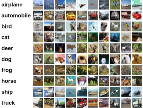
The CIFAR-10 dataset consists of 60,000 32x32 colour images in 10 classes, with 6000 images per class. There are 50,000 training images and 10,000 test images [39]. The amount of images of each class is equally distributed among the training and testing datasets, with 5000 and 1000 images per class respectively. Classes are mutually exclusive, meaning that each image cannot have more than one class. The different classes with some examples are shown in Figure 2.1.

Figure 2.1: Example images in each class (Source: The CIFAR-10 dataset)

We used the binary version available on the webpage, and converted it to the standard TensorFlow format called TFRecords. This way, it is easier to mix and match data sets and network architectures. The binary format is converted to an Example protocol buffer, then it is serialized to a string, and finally writes the string to a TFRecords file. This slightly reduces the amount of memory used by the dataset, but this conversion greatly benefits larger datasets.

(25)

By today’s standards, CIFAR-10 is a small dataset, compared to other ones available. MSCOCO has 2,500,000 labeled instances in 328,000 images for 91 different categories [44], ImageNet has 1.2 million training images with 1000 different classes [55] and Open Images has nearly 9 million images with over 6000 categories [37]. However, CIFAR-10 is a good enough dataset for proof of concept tasks, and is still commonly used as a benchmark. In this case, we are not aiming at state of the art results for this dataset, nor are we testing a new model architecture, but looking at the performance given different training methods. Thus, we con-sider this dataset to be good enough for our needs, as its size and training times should be generalizable to other cases.

2.2

Network architecture

For training our dataset, we use a relatively novel architecture presented by He et al. [28], called Residual Neural Networks (ResNets). As shown in Table 1.1, this architecture won the ImageNet classification and localization challenge in 2015, and enables to build much deeper networks than the ones trained until then. The reason to choose this architecture was that, in addition to be an interesting structure given the novelty, the original paper test the results on multiple datasets, including CIFAR-10, so we will have a base point for reference.

2.2.1

Residual Neural Networks

ResNets were created as an answer to the degradation problem observed when training very deep convolutional neural networks. As seen in section 1.3.2, deeper networks are crucial for better accuracy models, but some problems arises when trying to build deeper plain networks. Figure 2.2 shows how a plain deeper network performs worse than its shallower version.

Given that we just enlarge the network by adding layers that are identity mappings, there is no reason the deeper model should not perform as good as the shallow one. However, multiple tests demonstrate that there is an undesired behaviour, that generates a worse model. He et al. [28] argue that the problem seems not to be related to the notorious vanishing/exploding gradients, as this problem seems to have been largely addressed by normalized initialization of the layers, and intermediate normalization layers. They name the problematic as degradation, and found the main problem in the higher optimization difficulty of the more complex networks.

Figure 2.2: Comparison of plain networks and their residual counterparts in ImageNet. Thin lines denote training error and bold lines validation error. (Source: He et al. [28])

(26)

To solve this problematic they propose the addition of “shortcut connections”, as shown in Figure 2.3, that skip one or more layers, and do not add any extra parameter or computation complexity.

Figure 2.3: Residual learning building block. (Source: He [27])

They want to learn an underlying mapping H(x) by a few stacked layers, with x denoting the inputs to the first of these layers. With the hypothesis that multiple nonlinear layers can asymptotically approximate complicated functions, they assume that it will also asymptoti-cally approximate residual functions. Then instead of approximating H(x), they approximate F(x) := H(x)−x, with the original function becomingF(x) +x.

The idea is that given the case the identity is optimal, the solver may drive the weights of those layers to zero to approach the identity mappings. Although this may be a rare case, another case may be the optimal function is closer to an identity mapping than to a zero mapping, in which case it should be easier for the solver to find small fluctuations with reference to an identity mapping, than to learn the function as a new one.

The building block in Figure 2.3 can be defined as:

y=F(x,{Wi}) +x (2.1)

wherexandyare the inputs and output vectors of the layers considered. For the case where a shortcut connection is done between two layers with different dimensions, a linear projection Ws is done to match them:

y=F(x,{Wi}) +Wsx (2.2)

With this approach, He et al. [28] won the classification, localization and detection tracks on the ImageNet challenge, setting new state of the art results. In the classification track, they used a 152-layer network, with a block architecture that had lower complexity than VGG network with 16 or 19 layers. The final result of 3.57% top-5 error on the test set was obtained with the ensemble of six models of different depth (two of those six were 152-layer models). Unfortunately, no word on training times is provided in the original publication.

2.2.2

ResNet-56 with bottlenecks

The network we will implement for our tests will be one of the networks presented in He et al. [28], specifically built for testing CIFAR-10 dataset with ResNets. They test ResNets

(27)

with different depths, but follow the same pattern of blocks, just adding more repetitions of convolutions at multiple levels of depth.

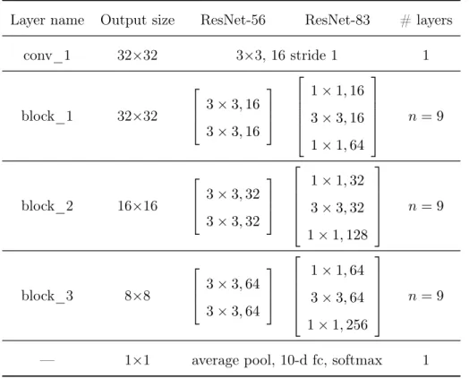
They work with inputs of 32×32, and feed them to a convolution with kernel height and width of size 3. Then they use a stack of 6n convolutions of the same kernel width and height as before, on feature maps of sizes {32,16,8}, with 2n layers in each feature map size and {16,32,64} filters respectively. The reduction of the map sizes is performed using convolutions with stride 2 at the end of each block, and the network ends with a global average pooling, a 10-way fully-connected layer, and a softmax, having a total of 6n+ 2 stacked weighted layers. The summary can be seen under the ResNet-56 column in Table 2.1, where the 56 layers are obtained with n = 9.

Table 2.1: ResNets summary

Layer name Output size ResNet-56 ResNet-83 # layers

conv_1 32×32 3×3, 16 stride 1 1 block_1 32×32    3×3,16 3×3,16          1×1,16 3×3,16 1×1,64       n= 9 block_2 16×16    3×3,32 3×3,32          1×1,32 3×3,32 1×1,128       n= 9 block_3 8×8    3×3,64 3×3,64          1×1,64 3×3,64 1×1,256       n= 9

— 1×1 average pool, 10-d fc, softmax 1

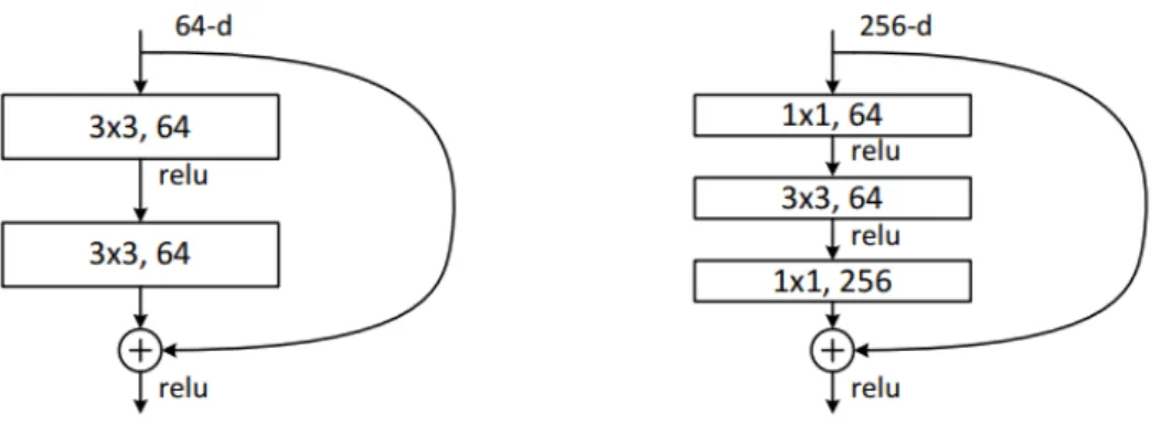
In the original paper they present an alternative building block with the name of “bottleneck” that they use in the ImageNet training networks, that can be seen at the right in Figure 2.4. This alternative architecture uses the 1×1 layers for reducing and increasing dimensionality of the network, while avoiding expensive computations of convolutions with higher kernel size and large number of filters

The final structure we are going to test in our servers is the one shown in the ResNet-83 column of the Table 2.1. We will usen = 9 with the bottlenecks blocks for a total of 83 layers. In order to built the model in TensorFlow we used a library, from the program itself, called TF-Slim [59]. This high level library contains the most common network architectures of the last years (AlexNet, VGG, Inception and ResNets), and also provides pretrained models for fine-tuning. The purpose of the library is to alleviate some of the tiring nomenclature TensorFlow uses when defining big models, and provide an easier programming model. However, it is a double-edged sword, because even though code can be simpler and easier to write, the extra layer can prevent full control of the model and customization the way it can be achieved with base TensorFlow.

(28)

Figure 2.4: “Bottleneck” building block used in ImageNet architectures. (Source: He et al. [28])

Training parameters

In the paper they specify the training configuration, that we will mostly replicate in our experiments. They use weight decay of λ= 0.0001, for regularizing the convolution layers, so that the regularizing term Ω(θ) = 1₂kwk2

2 is added to the objective function. TF-Slim is flexible enough for defining a general configuration that will be applied to all layers in our network, so we actually do not need to specify the parameters for each convolution, nor include the extra loss in our formula as this will be done automatically.

The optimizer will be gradient descent with Nesterov momentum [6] of 0.9, which is a first-order optimization method with better convergence rate guarantee than gradient descent in certain situations.

We will use the same layer initialization as they do in the original paper and that is de-scribed in He et al. [29]. It receives the name variance_scaling_initializer in TF-Slim, and improves the more common Xavier initialization [23] by taking into account the effect of rectifier nonlinearities. This enables them to train deeper models than using other more common initialization methods.

They use a batch size of 128 images, and begin with a learning rate of 0.1, dividing it by 10 at 32k and 48k iterations. It is possible to replicate this learning rate behavior in TensorFlow by usingtf.train.piecewise_constant, and defining the interval steps for each learning rate value. These values are not exactly the same as we used in our tests, as some of them were not working for our distributed configuration. They will be specified in the corresponding tests results in sections 3.2 and 3.3.

Our loss function will be the common cross entropy loss, which measures the probability error in discrete classification tasks in which the classes are mutually exclusive (each entry is in exactly one class). This is a common metric for classification problems in neural networks that works better for training purposes than plain accuracy or other formulas. Equation 2.3

computes the cross entropy between a true distribution pand an estimated distribution q.

H(p, q) =−X x

p(x) logq(x) (2.3)

The output of the softmax layer in our network would represent theq distribution, whereas the true labels will be one hot encoded vectors representing p. The final loss will be the mean value of the computed batch of images.

(29)

For data augmentation, we follow the same procedure for training: 4 pixel pad on each side of the image, and a 32×32 random crop, in addition of random horizontal flip. The testing dataset will not have any of those modifications.

2.3

Implemented architectures

We use the available implementation of ResNets in TF-Slim, and modify them to our par-ticular network, as the models published are specifically targeted at ImageNet data. We now explain the properties and the considerations of the two modes implemented in this project and whose results will be shown in the next chapter.

2.3.1

Asynchronous mode

The first mode we implemented is the fully asynchronous mode. As explained in section

1.4.1, the neural network will be replicated to each one of the workers that, after computing the gradients of the given batch, will update the model in the parameter servers asynchronously. The neural network will be replicated to each one of the workers, using the built-in function tf.train.replica_device_setter. This function is fed with the cluster definition, that is, the IP directions for the workers and the parameter servers as seen in section 1.5.3.

The function will take care to allocate the proper graph nodes to the correct device, thus model variables will be saved in parameter servers and sent to workers where they will be used for computing the whole model. The cluster definition will set which nodes are parameter servers and which are workers, so the framework efficiently lets the user focus on the model definition, as the correct assignment of variables will be done under the hood.

This method is straightforward for servers that only have a single GPU, as we can define a cluster inside the code with two parameter servers and three workers with the following parameters:

cluster_spec = {

"ps": ["nvb19-ib0:2222", "nvb20-ib0:2222"],

"worker": ["nvb21-ib0:2222", "nvb22-ib0:2222", "nvb23-ib0:2222"]}

However, using this definition in our servers would make the program to use a single GPU in each node, wasting big amounts of computational power. Therefore, we will use the environment variableCUDA_VISIBLE_DEVICESas a workaround to allocate 4 workers in a single server. Also, server direction can have different port numbers, so they are seen by the program as two different locations in the network. For instance, nvb21-ib0:2222 and nvb21-ib0:2223 are considered different directions on the same device, thus we can use it to our advantage to put multiple workers in a single server. The following example shows how we could manage to launch 2 workers (with indexes 0 to 1) and a parameter server on the same node:

CUDA_VISIBLE_DEVICES="" python script.py --ps_hosts=nvb19-ib0:2220 \

--worker_hosts=nvb19-ib0:2221,nvb19-ib0:2222 --job_name=ps --task_index=0 & \ CUDA_VISIBLE_DEVICES="0" python script.py --ps_hosts=nvb19-ib0:2220 \

--worker_hosts=nvb19-ib0:2221,nvb19-ib0:2222 --job_name=worker --task_index=0 & \ CUDA_VISIBLE_DEVICES="1" python script.py --ps_hosts=nvb19-ib0:2220 \

(30)

The parameter server has no available GPUs and all operations will be done using the CPUs. On the other hand, /job:worker/task:0 will only see the GPU with index 0 as the available device, so it can only allocate operations in the CPU and that specific GPU. Finally, /job:worker/task:1 will only see the GPU with index 1, as it is the index given to the CUDA_VISIBLE_DEVICES. As for the network directions, all of them point to node nvb19-ib0 (the -ib0 suffix is mandatory for all nodes given the platform protocol), but have different ports, thus will be seen as different nodes in the network. Table 2.2 summarizes the result of the call made above.

Table 2.2: Properties summary

Node Port Job name Task Index Available GPUs GPU index

nvb19-ib0 2220 ps 0 None —

nvb19-ib0 2221 worker 0 1 0

With this configuration we can put up to 4 workers in a single server, each with a different GPU, ensuring that all GPUs in the server are being used. If we want to apply this procedure in more than one node, we can use:

# In node nvb19

CUDA_VISIBLE_DEVICES="" python script.py --ps_hosts=nvb19-ib0:2220 \

--worker_hosts=nvb19-ib0:2221,nvb19-ib0:2222,nvb20-ib0:2221,nvb20-ib0:2222 \ --job_name=ps --task_index=0 & \

CUDA_VISIBLE_DEVICES="0" python script.py --ps_hosts=nvb19-ib0:2220 \

--worker_hosts=nvb19-ib0:2221,nvb19-ib0:2222,nvb20-ib0:2221,nvb20-ib0:2222 \ --job_name=worker --task_index=0 & \

--worker_hosts=nvb19-ib0:2221,nvb19-ib0:2222,nvb20-ib0:2221,nvb20-ib0:2222 \ --job_name=worker --task_index=1

# In node nvb20

--worker_hosts=nvb19-ib0:2221,nvb19-ib0:2222,nvb20-ib0:2221,nvb20-ib0:2222 \ --job_name=worker --task_index=2 & \

--worker_hosts=nvb19-ib0:2221,nvb19-ib0:2222nvb20-ib0:2221,nvb20-ib0:2222 \ --job_name=worker --task_index=3

The application Greasy will be the one in charge to run each line in the corresponding node, to make it work properly. This configuration generates 2 workers in each node with only one parameter server in the first one. Table 2.3 summarizes the properties for this case, and Figure 2.5 shows the schema.

Table 2.3: Properties summary

Node Port Job name Task Index Available GPUs GPU index

nvb19-ib0 2220 ps 0 None —

This is a straightforward method for easily distributing workers and parameter servers among multiple nodes, making the replication of the models in a way we can fully use all the

(31)

K80

worker_0 worker_1 PS_0 PS_0 nvb19

K80

worker_2 worker_3 nvb20

Figure 2.5: Schema for 2 nodes and 2 workers in each

available GPUs in the server for computing. The extent to which a parameter server in the same node can become a bottleneck is something that we will study more in depth in the next chapter. However, given the architecture of the MinoTauro this is the best way optimize the use of the servers, as allocating a full server only for this purpose will mean wasting a big amount of GPU resources.

2.3.2

Mixed asynchronous mode

As seen in the previous case, having multiple GPUs on the same server implies some con-straints when building our distributed models. The mixed asynchronous mode is more suited for our architecture, as we can use synchronous mode between GPUs on the same node, and asynchronously update the model between servers. In other words, we are using synchronous replicas intra-node and asynchronous replicas inter-node. However, deploying the model and gathering the statistics in each GPU is more complex than the previous mode, because device placement needs to be done at the code level manually which adds complexity to the overall process.

The cluster definition is similar as the one before, but in this case each worker will have 4 available GPUs, so we will only have a worker for each node, instead of the 4 we had in the fully asynchronous. This is how the call will look like, for allocating a single parameter server and a single worker in a unique node:

CUDA_VISIBLE_DEVICES="" python scipt.py \

--ps_hosts=nvb19-ib0:2220 --worker_hosts=nvb19-ib0:2221 \ --job_name=ps --task_index=0 & \

CUDA_VISIBLE_DEVICES="0,1,2,3" python scipt.py \

--ps_hosts=nvb19-ib0:2220 --worker_hosts=nvb19-ib0:2221 \ --job_name=worker --task_index=0

This worker will have all 4 GPUs available, and the model will be responsible for placing the clones in the corresponding GPU. The function for enforcing device placement constraints in TensorFlow is tf.device(), and we can specify a loop to place the model to all available GPUs. This process will be again replicated to multiple nodes using the

tf.train.replica_device_setter, and the total number of GPUs used will be the same. The key difference in this method is the way gradients are aggregated among all the clones in the node, which will make the iteration with a bigger effective size batch, improving the model.

(32)

The pseudocode in algorithm 1aims to provide a general understanding of the main part of the mixed asynchronous procedure that places and computes the model in the 4 GPUs available and the collects the losses and gradients in each one and reports it back to the parameter server. The Figure2.6 provides a general schema of a node with all the clones allocated.

1 for i in num_gpus do

2 with tf.device(’/job:worker/gpu:%d’ % i) do

3 clone_images, clone_labels ← get batch of data 4 predictions = model(clone_images)

5 clone_loss = cross_entropy(predictions, clone_labels) 6 clone_accuracy = accuracy(predictions, clone_labels)

7 end

8 end

9 grad_op ←create optimizer

10 grads_and_vars ←create empty list 11 clone_losses ← create empty list 12 for i in num_gpus do

13 with tf.device(’/job:worker/gpu:%d’ % i) do 14 clone_loss = get loss for clone i

15 scaled_clone_loss = clone_loss / num_gpus

16 clone_grad = compute gradients wrt trainable variables 17 append clone_grad to grads_and_vars

18 append scaled_clone_loss to clone_losses

19 end

20 end

21 total_loss = sum clone_losses

22 total_gradients = sum grads_and_vars

23 make the train_op apply the gradients in total_gradients

Algorithm 1: Clone allocation and gradient computation

K80

clone_0 clone_2 clone_3 clone_1 PS0 PS0 worker_0

(33)

2.4

Tools for assessing the model

As described in section 1.4, TensorFlow offers some tools to help during the training of the models. TensorBoard enables real-time monitoring of the running model, with a dashboard for following the evolution of the weights in the different layers during the training. Another interesting feature is the visualization of the operations defined in our model, as a full graph with interconnected nodes that represent each one of the operations declared in the code. It has different coloring options, so that nodes are colored according to their structure, or according to the device they are placed. For our case, this last option is the most interesting one, as we can assess if the device placement constraints we enforced in the code are correctly mapped.

Figure 2.7 shows the model build for the multi-GPU implementation. Inside the get_data node are all the operations related to loading and pre-processing the dataset. This node is then connected to the multiple clones, each one in a different GPU, as the colors in Figure2.8ashow. All the nodes that have not been given a specific device constraint will be placed in the fastest device available of either /job:worker/task:0 or /job:ps/task:0, as the get_data node. The top row of clones contains the operations for the backpropagation loop, with the gradient computations and nodes related to the optimization process that are built by the program.

Figure 2.7: Multi-GPU version ResNet-56 ops with device placement coloring

According to the color representation, each clone is placed on a different GPU, but parts of the model will be executed on/job:worker/task:0/gpu:0. If we navigate to the corresponding nodes, the batch normalization layers are responsible for this misconfiguration. Despite having enforced the correct GPU, the creation of those nodes in the code is beyond our working layer, so it is difficult to know if it is the intended configuration or not. However, we are able to trace another device misconfiguration related to the computation of accuracy and loss metrics, as shown in Figure 2.9a.

Those nodes are effectively placed by us, but a coding error in the indentation kept them out of the device placement constraint. The device they fall back by default is/job:worker/task:0, and more precisely /gpu:0, as it is the default device where TensorFlow ops will be allocated. Correcting the indentation and declaring the functions inside the corresponding device con-straint solved the placement problem, as seen in Figure 2.9b.

Other more in-depth tools for supervising device placement and node computation times is the Timeline tool. At a given step of the computation, we can output a JSON file that contains all the information of the executed operations for that step. It can help detect bottlenecks in

(34)

(a) Graph and color device legends

(b) Example of batch normalization layer device placement

Figure 2.8: TensorBoard screenshots

(a) Clone ops with unconstrained placement (b) Clone ops with constrained placement

(35)

operations, or again check whether the device placement is correct. Returning to the previous case, Figure2.10shows the Timeline for the case with the bad indentation and the misconfigured device placement for the metrics. /gpu:0 is working during all period, but the other GPUs are idle for some time between the 0.3s and 0.45s marks. The problem was the computation falling back to /gpu:0 made the models in other GPUs wait until they received the results. Solving the indentation problem solved the issue as seen in Figure 2.11, and idling times on GPUs is solved. However, the whole computation time has not been reduced, and /gpu:0 is still the bottleneck, mainly because it needs to compute extra operation for collecting all the gradients.

Figure 2.10: Tracing of the multi-GPU version ResNet-56 with unconstrained placement ops

Figure 2.11: Tracing of the multi-GPU version ResNet-56 with constrained placement ops

The Timelines showed above were obtained from a run in a single node, as the distributed version was still in development while writing this thesis, so no results of Timelines for dis-tributed versions could be generated. It was still possible to obtain the Timeline for a single node, as if it were in a local machine, but no stats of the global process could be gathered.

(36)

3. Results

This chapter shows the different kind of tests conducted in the platform. In the first section, short tests for depicting the scalability are shown, and in the second section the actual training runs are evaluated. All multinode tests are done using the asynchronous methods, as it is the only one fully working on the open source version of TensorFlow as the writing of this thesis.

3.1

Testing scalability

These tests were done using the workload explained in the previous section, with a ResNet-56 with bottleneck blocks (Figure 2.4) which increases its depth to 83 layers, and CIFAR-10 dataset. We evaluated each implementation with the same batch size, as we were testing the throughput of the system. The idea is that for distributed systems, larger batch sizes are more beneficial, as this requires less iterations per epoch, and we try to avoid network overheads as much as possible. According to Bengio [8], changing this hyperparameter will have a bigger impact on training times than on testing performance, although having fewer model updates per epoch will require visiting more examples in order to achieve the same error.

We also test different configurations of workers and parameter servers (PS), in order to be sure that the latter does not overcome a bottleneck when we increase the number of models that it receives and needs to update.

For reference, some scalability tests done in TensorFlow can be found at Abadi et al. [1], albeit they probably use the internal version deployed at Google servers. They test the scalabil-ity of training Inception-v3 using ImageNet dataset, with multiple replicas in both synchronous and asynchronous settings. In their server configurations each worker has 5 CPUs and 1 GPU (NVIDIA K40), whereas their parameter servers have 8 CPUs with no GPUs. Instead of show-ing multiple workshow-ing configurations of number of workers versus number of PS, they enable 17 PS for all tests, and modify the number of workers from 25 up to 200.

Our configuration is somewhat different, in the sense that all our servers have 4 NVIDIA K40 GPUs, so if we use a full server as a PS, we will be wasting 4 GPUs. Given the constraints of the architecture, we decided to allocate PS in the same nodes that contain the workers, but limiting their hardware use to only CPUs. As we did not know if that would be a limiting factor, we tried several configurations for both asynchronous and mixed-asynchronous workers, with the results shown in Figure 3.1.

The results are somewhat expected, as the fully asynchronous implementation is faster and scales better than the mixed-asynchronous. In the latter, the fact that losses and gradients need to be aggregated and processed generates some overhead that becomes more notorious as we increase the number of nodes. Take into account that in the asynchronous results we use each GPU as an independent worker, so total number of replicas will be 4, 8, 12, 16, 20, 24,

(37)

1 2 3 4 5 6 7 Nodes 0 500 1000 1500 2000 Images/sec 4 GPU 1PS async 4 GPU 2PS async 4 GPU 3PS async 4 GPU 1PS mixed-async 4 GPU 2PS mixed-async 4 GPU 3PS mixed-async

Figure 3.1: Tests of the workload in multiple server configurations.

28. In the mixed asynchronous case, there will be as much workers as number of nodes, and each will have 4 GPUs inside working in synchronous mode, but to the PS it would look as having 1, 2, 3, 4, 5, 6, 7 model replicas. Figures 2.5 and 2.6 in the previous section depict the hardware allocation of each mode.

If we look at the tests with different combinations of PS, there is no gain in using more than 1 PS, at least for the scale tested. The are some inconsistencies in the results when using more than 1 PS, and although we ran the tests at least two times, it is difficult to guess if these anomalies could be generated by a congested network, as other groups running jobs at MinoTauro use the same network. All in all, we did not observe any case in which the 1 PS server config