What Every Computer
Scientist
Should
Know About
Floating-Point
Arithmetic
DAVID GOLDBERG
Xerox Palo Alto Research Center, 3333 Coyote Hill Road, Palo Alto, CalLfornLa 94304
Floating-point arithmetic is considered an esotoric subject by many people. This is rather surprising, because floating-point is ubiquitous in computer systems: Almost every language has a floating-point datatype; computers from PCs to supercomputers have floating-point accelerators; most compilers will be called upon to compile
floating-point algorithms from time to time; and virtually every operating system must respond to floating-point exceptions such as overflow This paper presents a tutorial on the aspects of floating-point that have a direct impact on designers of computer systems. It begins with background on floating-point representation and rounding error, continues with a discussion of the IEEE floating-point standard, and concludes with examples of how computer system builders can better support floating point, Categories and Subject Descriptors: (Primary) C.0 [Computer Systems Organization]: General– instruction setdesign; D.3.4 [Programming Languages]:
Processors —compders, optirruzatzon; G.1.0 [Numerical Analysis]: General—computer arithmetic, error analysis, numerzcal algorithms (Secondary) D. 2.1 [Software Engineering]: Requirements/Specifications– languages; D, 3.1 [Programming
Languages]: Formal Definitions and Theory —semantZcs D ,4.1 [Operating Systems]: Process Management—synchronization
General Terms: Algorithms, Design, Languages
Additional Key Words and Phrases: denormalized number, exception, floating-point, floating-point standard, gradual underflow, guard digit, NaN, overflow, relative error, rounding error, rounding mode, ulp, underflow
INTRODUCTION
Builders of computer systems often need information about floating-point arith-metic. There are however, remarkably few sources of detailed information about it. One of the few books on the subject, Floating-Point Computation by Pat Ster-benz, is long out of print. This paper is a tutorial on those aspects of floating-point
arithmetic (floating-point hereafter) that have a direct connection to systems building. It consists of three loosely con-nected parts. The first (Section 1) dis-cusses the implications of using different rounding strategies for the basic
opera-tions of addition, subtraction, multipli-cation, and division. It also contains
background information on the two
methods of measuring rounding error, ulps and relative error. The second part discusses the IEEE floating-point stand-ard, which is becoming rapidly accepted by commercial hardware manufacturers. Included in the IEEE standard is the rounding method for basic operations; therefore, the discussion of the standard draws on the material in Section 1. The third part discusses the connections be-tween floating point and the design of various aspects of computer systems. Topics include instruction set design,
Permission to copy without fee all or part of this material is granted provided that the copies are not made or distributed for direct commercial advantage, the ACM copyright notice and the title of the publication and its data appear, and notice is given that copying is by permission of the Association for Computing Machinery. To copy otherwise, or to republish, requires a fee and/or specific permission.
@ 1991 ACM 0360-0300/91/0300-0005 $01.50
6 . David Goldberg
1 CONTENTS
INTRODUCTION 1 ROUNDING ERROR
1 1 Floating-Point Formats 12 Relatlve Error and Ulps 1 3 Guard Dlglts
14 Cancellation
1 5 Exactly Rounded Operations 2 IEEE STANDARD
2 1 Formats and Operations 22 S~eclal Quantltles
23 Exceptions, Flags, and Trap Handlers 3 SYSTEMS ASPECTS
3 1 Instruction Sets 32 Languages and Compders 33 Exception Handling 4 DETAILS
4 1 Rounding Error
42 Bmary-to-Decimal Conversion 4 3 Errors in Summatmn 5 SUMMARY
APPENDIX
ACKNOWLEDGMENTS REFERENCES
optimizing compilers, and exception handling.
All the statements made about float-ing-point are provided with justifications, but those explanations not central to the main argument are in a section called
The Details and can be skipped if
de-sired. In particular, the proofs of many of the theorems appear in this section. The end of each m-oof is marked with the H symbol; whe~ a proof is not included, the
❑ appears immediately following the statement of the theorem.
1. ROUNDING ERROR
Squeezing infinitely many real numbers into a finite number of bits requires an approximate representation. Although there are infinitely many integers, in most programs the result of integer com-putations can be stored in 32 bits. In contrast, given any fixed number of bits, most calculations with real numbers will produce quantities that cannot be exactly represented using that many bits. There-fore, the result of a floating-point calcu-lation must often be rounded in order to
fit back into its finite representation. The resulting rounding error is the character-istic feature of floating-point computa-tion. Section 1.2 describes how it is measured.
Since most floating-point calculations
have rounding error anyway, does it
matter if the basic arithmetic operations introduce a bit more rounding error than necessary? That question is a main theme throughout Section 1. Section 1.3 dis-cusses guard digits, a means of reducing the error when subtracting two nearby numbers. Guard digits were considered sufficiently important by IBM that in 1968 it added a guard digit to the double precision format in the System/360 ar-chitecture (single precision already had a guard digit) and retrofitted all existing machines in the field. Two examples are given to illustrate the utility of guard digits.
The IEEE standard goes further than just requiring the use of a guard digit. It gives an algorithm for addition, subtrac-tion, multiplication, division, and square root and requires that implementations produce the same result as that algo-rithm. Thus, when a program is moved from one machine to another, the results of the basic operations will be the same in every bit if both machines support the IEEE standard. This greatly simplifies the porting of programs. Other uses of this precise specification are given in Section 1.5.
2.1 Floating-Point Formats
Several different representations of real numbers have been proposed, but by far the most widely used is the floating-point representation.’ Floating-point represen-tations have a base O (which is always assumed to be even) and a precision p. If 6 = 10 and p = 3, the number 0.1 is rep-resented as 1.00 x 10⁻¹. If P = 2 and
P = 24, the decimal number 0.1 cannot
lExamples of other representations are floatzng slas;, aud szgned logan th m [Matula and Kornerup 1985; Swartzlander and Alexopoulos 1975]
Floating-Point Arithmetic ● 7
100X22 101X22 11 O X221.11X22
I I , ,
I [,!,1 r \ c r I i
o 1 2 3 4 5 6 7
Figure 1. Normalized numbers when (3 = 2,p = 3, em,n = – 1, emax = 2.
be represented exactly but is
approxi-mately 1.10011001100110011001101 x
2-4. In general, a floating-point num-ber will be represented as ~d. dd “ . . d
x /3’, where d. dd . . . d is called the significand2 and has p digits. More pre-cisely, kdO. dld2 “.” dp_l x b’ repre-sents the number
(
+ do + dl~-l + ““. +dP_l&(P-l))&, o<(il <~. (1)
The term floating-point number will
be used to mean a real number that can be exactly represented in the format un-der discussion. Two other parameters associated with floating-point represen-tations are the largest and smallest al-lowable exponents, e~~X and e~,~. Since there are (3P possible significands and emax — e~i. + 1 possible exponents, a floating-point number can be encoded in L(1°g2 ‘ma. – ‘m,. + 1)] + [log2((3J’)] + 1 its, where the final + 1 is for the sign bit. The precise encoding is not impor-tant for now.
There are two reasons why a real num-ber might not be exactly representable as a floating-point number. The most com-mon situation is illustrated by the deci-mal number 0.1. Although it has a finite decimal representation, in binary it has an infinite repeating representation. Thus, when D = 2, the number 0.1 lies strictly between two floating-point num-bers and is exactly representable by nei-ther of them. A less common situation is that a real number is out of range; that is, its absolute value is larger than f?x
2This term was introduced by Forsythe and Moler [196’71and has generally replaced the older term mantissa.
o
‘m= or smaller than 1.0 x ~em~. Most of this paper discusses issues due to the first reason. Numbers that are out of range will, however, be discussed in Sec-tions 2.2.2 and 2.2.4.Floating-point representations are not necessarily unique. For example, both 0.01 x 101 and 1.00 x 10⁻¹ represent 0.1. If the leading digit is nonzero [do # O in eq. (1)], the representation is said to be normalized. The floating-point num-ber 1.00 x 10⁻¹ is normalized, whereas 0.01 x 101 is not. When ~ = 2, p = 3,
e~i~ = – 1,and e~~X = 2, there are 16
normalized floating-point numbers, as shown in Figure 1. The bold hash marks correspond to numbers whose significant is 1.00. Requiring that a floating-point representation be normalized makes the representation unique. Unfortunately, this restriction makes it impossible to represent zero! A natural way to repre -sent O is with 1.0 x ~em~- 1, since this preserves the fact that the numerical or-dering of nonnegative real numbers cor-responds to the lexicographical ordering of their floating-point representations. 3 When the exponent is stored in a k bit field, that means that only 2 k – 1 values are available for use as exponents, since one must be reserved to represent O.
Note that the x in a floating-point number is part of the notation and differ-ent from a floating-point multiply
opera-tion. The meaning of the x symbol
should be clear from the context. For example, the expression (2.5 x 10⁻³, x
(4.0 X 10²) involves only a single float-ing-point multiplication.
3This assumes the usual arrangement where the exponent is stored to the left of the significant
8* David Goldberg
1.2 Relative Error and Ulps x /3’/~’+1. That is, Since rounding error is inherent in
float-:(Y’ s ;Ulp s ;6-’.
ing-point computation, it is important to (2)
have a way to measure this error. Con- 2
sider the floating-point format with ~ = ~
10 and p = 3, which will be used n particular, the relative error corre
-throughout this section. If the result of a spending to 1/2 ulp can vary by a factor floating-point computation is 3.12 x 10’2 ofSettingO. ThisE = (~ /2)~-Pfactor is calledto thethelargestwobble.of and the answer when computed to infi- the bounds in (2), we can say that when a nite precision is .0314, it is clear that real number is rounded to the closest this is in error by 2 units in the last floating-point number, the relative error place. Similarly, if the real number is always bounded by c, which is referred
.0314159 is represented as 3.14 x 10⁻², to as machine epsilon
then it is in error by .159 units in the In the example above, the relative er-last place. In general, if the floating-point ~or was .oo159i3, ~4159 = 0005. To avoid number d. d . . . d x fle is used to repre- such small numbers, the relative error is sent z, it is in error by Id. d . . . d–
( z//3’) I flp - 1units in the last place.4 The normally written as a factor times 6, term ulps will be used as shorthand for which5(10) -3 = .005.in this Thus,case isthe relativec = (~/2)P-Perror= “units in the last place. ” If the result of
a calculation is the floating-point num - would be expressed as ((.00159/ ber nearest to the correct result, it still 3.14159) /.oo5)eTo illustrate = O.l E.the difference between might be in error by as much as 1/2 ulp.
Another way to measure the difference ulps and relative error, consider the real between a floating-point number and the numberZ = 1.24 x 101. The error is 0.5 ulps; thex = 12.35. It is approximated by real number it is approximating is
rela-tive error, which is the difference be- relativecomputationerror8x. The exact value is 8 x =is 0.8 e. Next consider the tween the two numbers divided by the 98.8, whereas, the computed value is 81 real number. For example, the relative = 9.92 x 101. The error is now 4.0 ulps, error committed when approximating but the relative error is still 0.8 e. The 3.14159 by 3.14 x 10° is .00159 /3.14159
= .0005. error measured in ulps is eight times
To compute the relative error that cor- larger,the same. In general,even though the relativewhen the base is (3,error is responds to 1/2 ulp, observe that when a a fixed relative error expressed in ulps real number is approximated by the can wobble by a factor of up to (3. Con-closest possible floating-point number
P versely, as eq. (2) shows, a fixed error of
d dd ~. dd X ~e, the absolute error can be 1/2 ulps results in a relative error that
u can wobble by (3.
as large as ‘(Y x /3’ where & is The most natural way to measure
the digit ~/2. This error is ((~/2)&P) x rounding error is in ulps. For example, /3’ Since numb... of the form d. dd --- rounding to the neared flo~ting.point dd x /3eall have this same absolute error number corresponds to 1/2 ulp. When but have values that range between ~’ analyzing the rounding error caused by and Ox fle, the relative error ranges be- various formulas, however, relative error tween ((&/2 )~-’) x /3’//3’ and ((~/2)&J’) is a better measure. A good illustration
of this is the analysis immediately fol-lowing the proof of Theorem 10. Since ~ can overestimate the effect of rounding 4Un1ess the number z is larger than ~em=+ 1 or to the nearest floating-point number b; smaller than (lem~. Numbers that are out of range the wobble factor of (3, error estimates of in this fashion will not be considered until further formulas will be tighter on machines with
notice. a small p.
When only the order of magnitude of rounding error is of interest, ulps and e may be used interchangeably since they differ by at most a factor of ~. For exam-ple, when a floating-point number is in error by n ulps, that means the number of contaminated digits is logD n. If the relative error in a computation is ne, then
contaminated digits = log,n. (3)
1.3 Guard Digits
One method of computing the difference between two floating-point numbers is to compute the difference exactly, then round it to the nearest floating-point number. This is very expensive if the operands differ greatly in size. Assuming P = 3, 2,15 X 10¹² – 1.25 X 10⁻⁵ would be calculated as
x = 2.15 X 10¹²
y = .0000000000000000125 X 1012
X – y = 2.1499999999999999875 X 10¹²,
which rounds to 2.15 x 10¹². Rather than using all these digits, floating-point hardware normally operates on a fixed number of digits. Suppose the number of
digits kept is p and that when the
smaller operand is shifted right, digits
are simply discarded (as opposed to
rounding). Then, 2.15 x 10¹² – 1.25 x 10⁻⁵ becomes
x = 2.15 X 10¹² ‘y = 0.00 x 10¹² x–y =2.15x10¹².
The answer is exactly the same as if the difference had been computed exactly then rounded. Take another example: 10.1 – 9.93. This becomes
x= 1.01 x 101 ‘y = 0.99 x 101 X–yz .02 x 101.
The correct answer is .17, so the com-puted difference is off by 30 ulps and is
Floating-Point Arithmetic g 9
wrong in every digit! How bad can the error be?
Theorem 1
Using a floating-point format with pa-rameters /3 and p and computing differ-ences using p digits, the relative error of the result can be as large as b – 1.
Proofi A relative error of 13– 1 in
the expression x – y occurs when x = 1.00””” Oandy=. pp. ””p, wherep= @ – 1. Here y has p digits (all equal to Q). The exact difference is x – y = P ‘p. When computing the answer using only p digits, however, the rightmost digit of y gets shifted off, so the computed
differ-ence is P–p+l. Thus, the error is p-p – @-P+l = ~-P(~ – 1), and the relative er-ror is $-P((3 – l)/O-p = 6 – 1. H
When f? = 2, the absolute error can be as large as the result, and when 13= 10, it can be nine times larger. To put it another way, when (3 = 2, (3) shows that the number of contaminated digits is log2(l/~) = logJ2 J’) = p. That is, all of the p digits in the result are wrong!
Suppose one extra digit is added to guard against this situation (a guard digit). That is, the smaller number is truncated to p + 1 digits, then the result of the subtraction is rounded to p digits. With a guard digit, the previous example becomes
x = 1.010 x 101 y = 0.993 x 101
x–y= .017 x 101,
and the answer is exact. With a single guard digit, the relative error of the re -suit may be greater than ~, as
8.59:
x= 1.1OX 102
y = .085 X 102
z–y= 1.015 x 10²
This rounds to 102, compared
in 110 –
with the correct answer of 101.41, for a relative error of .006, which is greater than
10 “ David Goldberg
e = .005. In general, the relative error of the result can be only slightly larger than c. More precisely, we have Theorem 2.
Theorem 2
If x and y are floating-point numbers in a format with 13 and p and if subtraction is done with p + 1 digits (i. e., one guard digit), then the relative rounding error in the result is less than 2 ~.
This theorem will be proven in Section 4.1. Addition is included in the above theorem since x and y can be positive or negative.
1.4 Cancellation
Section 1.3 can be summarized by saying that without a guard digit, the relative error committed when subtracting two nearby quantities can be very large. In other words, the evaluation of any ex-pression containing a subtraction (or an addition of quantities with opposite signs) could result in a relative error so large that all the digits are meaningless (The-orem 1). When subtracting nearby quan-tities, the most significant digits in the operands match and cancel each other. There are two kinds of cancellation: catastrophic and benign.
Catastrophic cancellation occurs when the operands are subject to rounding er-rors. For example, in the quadratic for-mula, the expression bz – 4 ac occurs. The quantities 62 and 4 ac are subject to rounding errors since they are the re-sults of floating-point multiplications. Suppose they are rounded to the nearest floating-point number and so are accu-rate to within 1/2 ulp. When they are subtracted, cancellation can cause many of the accurate digits to disappear, leav-ing behind mainly digits contaminated by rounding error. Hence the difference might have an error of many ulps. For example, consider b = 3.34, a = 1.22, and c = 2.28. The exact value of b2 --4 ac is .0292. But b2 rounds to 11.2 and 4ac rounds to 11.1, hence the final an-swer is .1, which is an error by 70 ulps even though 11.2 – 11.1 is exactly equal
to .1. The subtraction did not introduce any error but rather exposed the error introduced in the earlier multiplications.
Benign cancellation occurs when sub-tracting exactly known quantities. If x and y have no rounding error, then by Theorem 2 if the subtraction is done with a guard digit, the difference x – y has a very small relative error (less than 2 e).
A formula that exhibits catastrophic cancellation can sometimes be rear-ranged to eliminate the problem. Again consider the quadratic formula
–b+ ~b2–4ac
–b–~ r2 =
2a “
(4)
When b2 P ac, then b2 – 4 ac does not
involve a cancellation and ~ =
\b 1.But the other addition (subtraction) in one of the formulas will have a catas-trophic cancellation. To avoid this, mul-tiply the numerator and denominator of
r-l by – b – ~ (and similarly
for r2 ) to obtain
2C rl =
–b–~’ 2C rz =
–b+~”
(5)
If b2 % ac and b >0, then computing rl using formula (4) will involve a cancella-tion. Therefore, use (5) for computing rl and (4) for rz. On the other hand, if b <0, use (4) for computing rl and (5) for r2.
The expression X2 – y2 is another for-mula that exhibits catastrophic cancella-tion. It is more accurate to evaluate it as ( x – y)( x + y). 5 Unlike the quadratic
5Although the expression ( x – .Y)(x + y) does not cause a catastrophic cancellation, it IS shghtly less accurate than X2 – y2 If x > y or x < y In this case, ( x – -Y)(x + y) has three rounding errors, but X2 – y2 has only two since the rounding error com-mitted when computing the smaller of x 2 and y 2 does not affect the final subtraction.
Floating-Point Arithmetic 8 11
formula, this improved form still has a subtraction, but it is a benign cancella-tion of quantities without rounding er-ror, not a catastrophic one. By Theorem 2, the relative error in x – y is at most 2 e. The same is true of x + y. Multiply-ing two quantities with a small relative error results in a product with a small relative error (see Section 4.1).
To avoid confusion between exact and computed values, the following notation is used. Whereas x – y denotes the exact difference of x and y, x @y denotes the computed difference (i. e., with rounding error). Similarly @, @, and @ denote computed addition, multiplication, and division, respectively. All caps indicate the computed value of a function, as in LN( x) or SQRT( x). Lowercase functions and traditional mathematical notation denote their exact values as in ln( x) and &.
Although (x @y) @ (x @ y) is an ex-cellent approximation of x 2 – y2, the floating-point numbers x and y might themselves be approximations to some true quantities 2 and j. For example, 2 and j might be exactly known decimal numbers that cannot be expressed ex-actly in binary. In this case, even though x ~ y is a good approximation to x – y, it can have a huge relative error com-pared to the true expression 2 – $, and so the advantage of ( x + y)( x – y) over X2 – y2 is not as dramatic. Since comput -ing ( x + y)( x – y) is about the same amount of work as computing X2 – y2, it is clearly the preferred form in this case. In general, however, replacing a catas-trophic cancellation by a benign one is not worthwhile if the expense is large because the input is often (but not al-ways) an approximation. But eliminat -ing a cancellation entirely (as in the quadratic formula) is worthwhile even if the data are not exact. Throughout this paper, it will be assumed that the float-ing-point inputs to an algorithm are ex -.aGtand Qxat the results are computed as accurately as possible.
The expression X2 – y2 is more accu-rate when rewritten as (x – y)( x + y) because a catastrophic cancellation is
replaced with a benign one. We next pre-sent more interesting examples of formu-las exhibiting catastrophic cancellation that can be rewritten to exhibit only benign cancellation.
The area of a triangle can be expressed directly in terms of the lengths of its sides a, b, and c as
A = ~s(s - a)(s - b)(s - c) ,
a+b+c where s =
2 . (6)
Suppose the triangle is very flat; that is,
a = b + c. Then s = a, and the term
(s – a) in eq. (6) subtracts two nearby numbers, one of which may have round-ing error. For example, if a = 9.0, b = c
= 4.53, then the correct value of s is
9.03 and A is 2.34. Even though the
computed value of s (9.05) is in error by only 2 ulps, the computed value of A is 3.04, an error of 60 ulps.
There is a way to rewrite formula (6) so that it will return accurate results even for flat triangles [Kahan 1986]. It is A= [(la+ (b+c))(c - (a-b))
X(C+ (a– b))(a+ (b– c))] ’/’/4,
a? b?c. (7)
If a, b, and c do not satisfy a > b > c, simply rename them before applying (7). It is straightforward to check that the right-hand sides of (6) and (7) are alge-braically identical. Using the values of a, b, and c above gives a computed area of 2.35, which is 1 ulp in error and much more accurate than the first formula.
Although formula (7) is much more
accurate than (6) for this example, it would be nice to know how well (7) per-forms in general.
Theorem 3
The rounding error incurred when using (T) #o compuie the area of a t.icqqle ie at most 11 e, provided subtraction is per-formed with a guard digit, e <.005, and square roots are computed to within 1/2 Ulp.
12 “ David Goldberg
The condition that c s .005 is met in virtually every actual floating-point sys-tem. For example, when 13= 2, p >8 ensures that e < .005, and when 6 = 10, p z 3 is enough.
In statements like Theorem 3 that dis-cuss the relative error of an expression, it is understood that the expression is computed using floating-point arith-metic. In particular, the relative error is actually of the expression
The troublesome expression (1 + i/n)’ can be rewritten as exp[ n ln(l + i / n)], where now the problem is to compute In(l + x) for small x. One approach is to use the approximation ln(l + x) = x, in
which case the payment becomes
$37617.26, which is off by $3.21 and even less accurate than the obvious formula. But there is a way to compute ln(l + x)
accurately, as Theorem 4 shows
[Hewlett-Packard 1982], This formula yields $37614.07, accurate to within 2
(sQRT(a @(b @c))@ (C @(a @b))
cents!
Theorem 4 assumes that LN( x)ap-F3(c @(a @b))@ (a @(b @c))) proximateproblem it solves is that whenln( x) to within 1/2 ulp.x is small,The
@4. (8) LN(l @ x) is not close to ln(l + x)
be-cause 1 @ x has lost the information in the low order bits of x. That is, the com-Because of the cumbersome nature of (8), puted value of ln(l + x) is not close to its in the statement of theorems we will actual value when x < 1.
usually say the computed value of E
rather than writing out E with circle Theorem 4 notation.
Error bounds are usually too
pes-simistic. In the numerical example given above, the computed value of (7) is 2.35, compared with a true value of 2.34216 for a relative error of O.7c, which is much less than 11 e. The main reason for com-puting error bounds is not to get precise bounds but rather to verify that the formula does not contain numerical problems.
A final example of an expression that can be rewritten to use benign cancella-tion is (1 + x)’, where x < 1. This ex-pression arises in financial calculations. Consider depositing $100 every day into a bank account that earns an annual interest rate of 6~o, compounded daily. If
n = 365 and i = ,06, the amount of
money accumulated at the end of one
year is 100[(1 + i/n)” – 11/(i/n) dol-lars. If this is computed using ~ = 2 and P = 24, the result is $37615.45 compared
to the exact answer of $37614.05, a
discrepancy of $1.40. The reason for the problem is easy to see. The
expres-sion 1 + i/n involves adding 1 to
.0001643836, so the low order bits of i/n are lost. This rounding error is amplified when 1 + i / n is raised to the nth power.
If ln(l – x) is computed using the for-mula
ln(l + x)
I
x forl~x=l— —
1
xln(l + x)(1 +X)-1 forl G3x#l
the relative error is at most 5 c when O < x < 3/4, provided subtraction is per-formed with a guard digit, e <0.1, and in is computed to within 1/2 ulp.
This formula will work for any value of x but is only interesting for x + 1, which is where catastrophic cancellation occurs in the naive formula ln(l + x) Although the formula may seem mysterious, there is a simple explanation for why it works. Write ln(l + x) as x[ln(l + x)/xl = XV(x). The left-hand factor can be com-puted exactly, but the right-hand factor P(x) = ln(l + x)/x will suffer a large rounding error when adding 1 to x. How-ever, v is almost constant, since ln(l + x) = x. So changing x slightly will not introduce much error. In other words, if z= x, computing XK( 2) will be a good
Floating-Point Arithmetic 8 13
approximation to xp( x) = ln(l + x). Is
there a value for 5 for which 2 and
5 + 1 can be computed accurately? There is; namely, 2 = (1 @ x) e 1, because then 1 + 2 is exactly equal to 1 @ x.
The results of this section can be sum-marized by saying that a guard digit guarantees accuracy when nearby pre-cisely known quantities are subtracted (benign cancellation). Sometimes a for-mula that gives inaccurate results can be rewritten to have much higher numeri -cal accuracy by using benign cancella-tion; however, the procedure only works if subtraction is performed using a guard digit. The price of a guard digit is not high because is merely requires making the adder 1 bit wider. For a 54 bit double precision adder, the additional cost is less than 2%. For this price, you gain the ability to run many algorithms such as formula (6) for computing the area of a triangle and the expression in Theorem 4 for computing ln(l + ~). Although most modern computers have a guard digit, there are a few (such as Crays) that do not.
1.5 Exactly Rounded Operations
When floating-point operations are done with a guard digit, they are not as accu-rate as if they were computed exactly then rounded to the nearest floating-point number. Operations performed in this manner will be called exactly rounded.
The example immediately preceding
Theorem 2 shows that a single guard digit will not always give exactly rounded results. Section 1.4 gave several exam-ples of algorithms that require a guard digit in order to work properly. This sec-tion gives examples of algorithms that require exact rounding.
So far, the definition of rounding has not been given. Rounding is straightfor-ward, with the exception of how to round halfway cases; for example, should 12.5 mnnd to 12 OP 12? Ofie whool of thought divides the 10 digits in half, letting {0, 1,2,3,4} round down and {5,6,’7,8,9} round up; thus 12.5 would round to 13. This is how rounding works on Digital
Equipment Corporation’s VAXG comput -ers. Another school of thought says that since numbers ending in 5 are halfway between two possible roundings, they
should round down half the time and
round up the other half. One way of ob -taining this 50’%0behavior is to require that the rounded result have its least
significant digit be even. Thus 12.5 rounds to 12 rather than 13 because 2 is even. Which of these methods is best, round up or round to even? Reiser and Knuth [1975] offer the following reason for preferring round to even.
Theorem 5
Let x and y be floating-point numbers,
and define X. = x, xl=(xOey)O
y,...,=(x(ley)@y)If@If@ and
e are exactly rounded using round to
even, then either x. = x for all n or x. = xl foralln >1. ❑
To clarify this result, consider ~ = 10,
p = 3 and let x = 1.00, y = –.555.
When rounding up, the sequence
be-comes X. 9 Y = 1.56, Xl = 1.56 9 .555 = 1.01, xl e y ~ LO1 Q .555 = 1.57, and each successive value of x. in-creases by .01. Under round to even, x. is always 1.00. This example suggests that when using the round up rule, com-putations can gradually drift upward, whereas when using round to even the
theorem says this cannot happen.
Throughout the rest of this paper, round to even will be used.
One application of exact rounding oc-curs in multiple precision arithmetic. There are two basic approaches to higher precision. One approach represents float -ing-point numbers using a very large sig-nificant, which is stored in an array of words, and codes the routines for manip-ulating these numbers in assembly lan-guage. The second approach represents higher precision floating-point numbers as an array of ordinary floating-point
‘VAX is a trademark of Digital Equipment Corporation.
14 “ David Goldberg
numbers, where adding the elements of the array in infinite precision recovers the high precision floating-point number. It is this second approach that will be discussed here. The advantage of using an array of floating-point numbers is that it can be coded portably in a high-level language, but it requires exactly rounded arithmetic.
The key to multiplication in this sys-tem is representing a product xy as a sum, where each summand has the same precision as x and y. This can be done by splitting x and y. Writing x = x~ + xl and y = y~ + yl, the exact product is xy = xhyh + xhyl + Xlyh + Xlyl. If X and y have p bit significands, the summands will also have p bit significands, pro-vided XI, xh, yh? Y1 carI be represented using [p/2] bits. When p is even, it is easy to find a splitting. The number Xo. xl ““” xp_l can be written as the sum of Xo. xl ““” xp/2–l and O.O.. .OXP,Z . . . XP ~. When p is odd, this simple splitting method will not work. An extra bit can, however, be gained by using neg-ative numbers. For example, if ~ = 2, P = 5, and x = .10111, x can be split as x~ = .11 and xl = – .00001. There is more than one way to split a number. A splitting method that is easy to compute is due to Dekker [1971], but it requires more than a single guard digit.
Theorem 6
Let p be the floating-point precision, with the restriction that p is even when D >2,
ulps. Using Theorem 6 to write b = 3.5
– .024, a = 3.5 – .037, and c = 3.5 –
.021, b2 becomes 3.52 – 2 x 3.5 x .024 + .0242. Each summand is exact, so b2 = 12.25 – .168 + .000576, where the sum is left unevaluated at this point. Similarly,
ac = 3.52 – (3.5 x .037 + 3.5 x .021) + .037 x .021
= 12.25 – .2030 + .000777.
Finally, subtracting these two series term by term gives an estimate for b2 – ac of
O @ .0350 e .04685 = .03480, which is
identical to the exactly rounded result. To show that Theorem 6 really requires exact rounding, consider p = 3, P = 2,
and x = 7. Then m = 5, mx = 35, and
m @ x = 32. If subtraction is performed with a single guard digit, then (m @ x)
e x = 28. Therefore, x~ = 4 and xl = 3, ~~e xl not representable with \p/2] =
As a final example of exact rounding, consider dividing m by 10. The result is a floating-point number that will in gen-eral not be equal to m/10. When P = 2, however, multiplying m @10 by 10 will miraculously restore m, provided exact rounding is being used. Actually, a more general fact (due to Kahan) is true. The proof is ingenious, but readers not inter-ested in such details can skip ahead to Section 2.
and assume that fl;ating-point operations are exactly rounded. Then if k = ~p /2~ is half the precision (rounded up) and m = fik + 1, x can je split as x = Xh + xl,
where xh=(m Q9x)e (m@ Xe x), xl
—
— x e Xh, and each x, is representable using ~p/2] bits of precision.
To see how this theorem works in an example, let P = 10, p = 4, b = 3.476,
a = 3.463, and c = 3.479. Then b2 – ac
rounded to the nearest floating-point number is .03480, while b @ b = 12.08, a @ c = 12.05, and so the computed value of b2 – ac is .03. This is an error of 480
Theorem 7
When O = 2, if m and n are integers with ~m ~ < 2p-1 and n has the special form
n=2z+2J then (m On)@n=m,
provided fi?~ating-point operations are exactly rounded.
Proof Scaling by a power of 2 is
harmless, since it changes only the expo-nent not the significant. If q = m /n, then scale n so that 2P-1 s n < 2P and scale m so that 1/2 < q < 1. Thus, 2P–2 < m < 2P. Since m has p significant bits, it has at most 1 bit to the right of the binary point. Changing the sign of m
is harmless, so assume q > 0.
Floating-Point Arithmetic g 15
If ij = m @ n, to prove the theorem requires showing that
That is because m has at most 1 bit right of the binary point, so nij will round to
m. TO deal with the halfway case when
I T@ – m I = 1/4, note that since the ini-tial unscaled m had Im I < 2‘- 1, its low-order bit was O, so the low-order bit of the scaled m is also O. Thus, halfway cases will round to m.
Suppose q = .qlqz “.. , and & g = . . . qP1. To estimate Inq – m 1, ifs? compute I ~ – q I = IN/2p+1 –
m/nl, where N is an odd integer.
Since n=2’+2J and 2P-l <n <2p, it must be that n = 2P–1 + 2k for some ~ < p – 2, and thus
(2~-’-k
+
~)N- ~p+l-km ——
n~p+l–k
The numerator is an integer, and since N is odd, it is in fact an odd integer. Thus, I ~ – q ] > l/(n2P+l-k). Assume q < @(the case q > Q is similar). Then nij < m, and
Im-n@l= m-nij=n(q-@)
= n(q – (~ – 2-P-1))
(
1 < n 2–P–1 —
n2 p+1–k )
= (2 P-1 +2’)2-’-’ +2-P-’+’=:.
This establishes (9) and proves the
theo-rem. ❑
The theorem holds true for any base 6, as long as 2 z + 2 J is replaced by (3L + DJ. As 6 gets larger. however, there are
fewer and fewer denominators of the
form ~’ + p’.
We are now in a position to answer the question, Does it matter if the basic
arithmetic operations introduce a little more rounding error than necessary? The answer is that it does matter, because accurate basic operations enable us to prove that formulas are “correct” in the sense they have a small relative error. Section 1.4 discussed several algorithms that require guard digits to produce cor-rect results in this sense. If the input to those formulas are numbers representing imprecise measurements, however, the bounds of Theorems 3 and 4 become less interesting. The reason is that the
be-nign cancellation x – y can become
catastrophic if x and y are only approxi-mations to some measured quantity. But accurate operations are useful even in the face of inexact data, because they enable us to establish exact relationships like those discussed in Theorems 6 and 7. These are useful even if every floating-point variable is only an approximation to some actual value.
2. IEEE STANDARD
There are two different IEEE standards for floating-point computation. IEEE 754 is a binary standard that requires P = 2, p = 24 for single precision and p = 53 for double precision [IEEE 19871. It also specifies the precise layout of bits in a single and double precision. IEEE 854 allows either L?= 2 or P = 10 and unlike 754, does not specify how floating-point numbers are encoded into bits [Cody et al. 19841. It does not require a particular value for p, but instead it specifies con-straints on the allowable values of p for single and double precision. The term
IEEE Standard will be used when
dis-cussing properties common to both
standards.
This section provides a tour of the IEEE standard. Each subsection discusses one aspect of the standard and why it was included. It is not the purpose of this paper to argue that the IEEE standard is the best possible floating-point standard but rather to accept the standard as given and provide an introduction to its use. For full details consult the standards [Cody et al. 1984; Cody 1988; IEEE 19871.
16 ● David Goldberg
2.1 Formats and Operations 2. 1.1 Base
It is clear why IEEE 854 allows ~ = 10.
Base 10 is how humans exchange and
think about numbers. Using (3 = 10 is especially appropriate for calculators, where the result of each operation is dis-played by the calculator in decimal.
There are several reasons w~y IEEE 854 requires that if the base is not 10, it must be 2. Section 1.2 mentioned one reason: The results of error analyses are
much tighter when ~ is 2 because a
rounding error of 1/2 ulp wobbles by a factor of fl when computed as a relative error, and error analyses are almost al-ways simpler when based on relative er-ror. A related reason has to do with the effective precision for large bases. Con-sider fi = 16, p = 1 compared to ~ = 2, p = 4. Both systems have 4 bits of signif-icant. Consider the computation of 15/8. When ~ = 2, 15 is represented as 1.111
x 23 and 15/8 as 1.111 x 2°, So 15/8 is exact. When p = 16, however, 15 is rep-resented as F x 160, where F is the hex-adecimal digit for 15. But 15/8 is repre-sented as 1 x 160, which has only 1 bit correct. In general, base 16 can lose up to 3 bits, so a precision of p can have an effective precision as low as 4p – 3 rather than 4p.
Since large values of (3 have these problems, why did IBM choose 6 = 16 for its system/370? Only IBM knows for sure, but there are two possible reasons. The first is increased exponent range. Single precision on the system/370 has ~ = 16, p = 6. Hence the significant requires 24 bits. Since this must fit into 32 bits, this leaves 7 bits for the exponent and 1 for the sign bit. Thus, the magnitude of rep-resentable numbers ranges from about 16-2’ to about 1626 = 228. To get a simi-lar exponent range when D = 2 would require 9 bits of exponent, leaving only 22 bits for the significant. It was just pointed out, however, that when D = 16, the effective precision can be as low as 4p – 3 = 21 bits. Even worse, when B = 2 it is possible to gain an extra bit of
precision (as explained later in this sec-tion), so the ~ = 2 machine has 23 bits of precision to compare with a range of 21-24 bits for the ~ = 16 machine.
Another possible explanation for
choosing ~ = 16 bits has to do with shift-ing. When adding two floating-point numbers, if their exponents are different, one of the significands will have to be shifted to make the radix points line up, slowing down the operation. In the /3 =
16, p = 1 system, all the numbers
be-tween 1 and 15 have the same exponent, so no shifting is required when adding any of the
()15 = 105 possible pairs of distinct numb~rs from this set. In the b = 2, P = 4 system, however, these numbers have exponents ranging from O to 3, and shifting is required for 70 of the
105 pairs.
In most modern hardware, the perform-ance gained by avoiding a shift for a subset of operands is negligible, so the
small wobble of (3 = 2 makes it the
preferable base. Another advantage of using ~ = 2 is that there is a way to gain an extra bit of significance .V Since float-ing-point numbers are always normal-ized, the most significant bit of the significant is always 1, and there is no reason to waste a bit of storage repre-senting it. Formats that use this trick are said to have a hidden bit. It was pointed out in Section 1.1 that this re-quires a special convention for O. The method given there was that an expo-nent of e~,~ – 1 and a significant of all zeros represent not 1.0 x 2 ‘mln–1 but rather O.
IEEE 754 single precision is encoded in 32 bits using 1 bit for the sign, 8 bits for the exponent, and 23 bits for the sig-nificant. It uses a
so the significant even though it is 23 bits.
hidden bit, howeve~, is 24 bits (p = 24), encoded using only
‘This appears to have first been published by Gold-berg [1967], although Knuth [1981 page 211] at-tributes this Idea to Konrad Zuse
Floating-Point Arithmetic ● 17
2. 1.2 Precision
The IEEE standard defines four different precision: single, double, single ex-tended, and double extended. In 754, sin-gle and double precision correspond roughly to what most floating-point hardware provides. Single precision oc-cupies a single 32 bit word, double
preci-sion two consecutive 32 bit words.
Extended precision is a format that offers just a little extra precision and exponent
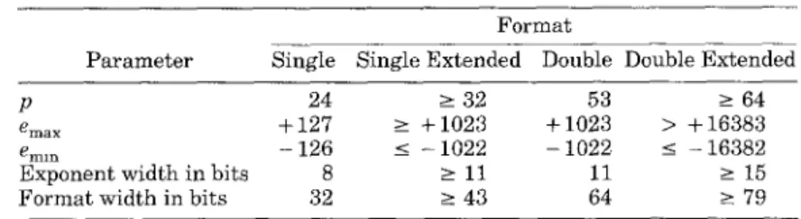
range (Table 1). The IEEE standard only specifies a lower bound on how many extra bits extended precision provides. The minimum allowable double-extended format is sometimes referred to as 80-bit format, even though the table shows it using 79 bits. The reason is that hard-ware implementations of extended preci-sion normally do not use a hidden bit and so would use 80 rather than 79 bits.8
The standard puts the most emphasis on extended precision, making no recom-mendation concerning double precision but strongly recommending that
Implementations should support the extended format corresponding to the widest basic format supported,
One motivation for extended precision comes from calculators, which will often display 10 digits but use 13 digits inter-nally. By displaying only 10 of the 13 digits, the calculator appears to the user ~ } a black box that computes exponen-tial, cosines, and so on, to 10 digits of accuracy. For the calculator to compute functions like exp, log, and cos to within
10 digits with reasonable efficiency, how-ever, it needs a few extra digits with which to work. It is not hard to find a simple rational expression that approxi-mates log with an error of 500 units in the last place. Thus, computing with 13 digits gives an answer correct to 10 dig-its. By keeping these extra 3 digits
hid-*According to Kahan, extended precision has 64 bits of significant because that was the widest precision across which carry propagation could be done on the Intel 8087 without increasing the cycle time [Kahan 19881.
den, the calculator presents a simple model to the operator.
Extended precision in the IEEE stand-ard serves a similar function. It enables libraries to compute quantities to within about 1/2 ulp in single (or double) preci-sion efficiently, giving the user of those libraries a simple model, namely, that each primitive operation, be it a simple multiply or an invocation of log, returns a value accurate to within about 1/2 ulp. When using extended precision, however, it is important to make sure that its use is transparent to the user. For example, on a calculator, if the internal represen-tation of a displayed value is not rounded to the same precision as the display, the result of further operations will depend on the hidden digits and appear unpre-dictable to the user.
To illustrate extended precision fur-ther, consider the problem of converting between IEEE 754 single precision and decimal. Ideally, single precision num-bers will be printed with enough digits so that when the decimal number is read back in, the single precision number can be recovered. It turns out that 9 decimal digits are enough to recover a single pre-cision binary number (see Section 4.2). When converting a decimal number back to its unique binary representation, a rounding error as small as 1 ulp is fatal because it will give the wrong answer. Here is a situation where extended preci-sion is vital for an efficient algorithm. When single extended is available, a straightforward method exists for con-verting a decimal number to a single precision binary one. First, read in the 9 decimal digits as an integer N, ignoring the decimal point. From Table 1, p >32, and since 109 < 232 = 4.3 x 10⁹, N can be represented exactly in single ex-tended. Next, find the appropriate power 10P necessary to scale N. This will be a combination of the exponent of the
deci-mal number, and the position of the
(up until now) ignored decimal point. Compute 10 I ‘l. If \P I s 13, this is also represented exactly, because 1013 = 213513 and 513<232. Finally, multiply (or divide if P < 0) N and 10’ P‘. If this
18 - David Goldberg
Table 1. IEEE 754 Format Parameters Format
Parameter Single Single Extended Double Double Extended
P 24 > 32 53 > 64
emax + 127 z + 1023 + 1023 > + 16383 emln – 126 < – 1022 – 1022 < – 163$32 Exponent width in bits 8 > 11 11 2 15
Format width in bits 32 2 43 64 2 79
last operation is done exactly, the closest binary number is recovered. Section 4.2 shows how to do the last multiply (or divide) exactly. Thus, for IP I s 13, the use of the single-extended format enables 9 digit decimal numbers to be converted to the closest binary number (i. e., ex-actly rounded). If IP I > 13, single-extended is not enough for the above algorithm to compute the exactly rounded binary equivalent always, but Coonen [1984] shows that it is enough to guaran-tee that the conversion of binary to deci-mal and back will recover the original binary number.
If double precision is supported, the algorithm above would run in double precision rather than single-extended, but to convert double precision to a 17 digit decimal number and back would require the double-extended format.
2.1.3 Exponent
Since the exponent can be positive or negative, some method must be chosen to represent its sign. Two common methods
of representing signed numbers are
sign/magnitude and two’s complement. Sign/magnitude is the system used for the sign of the significant in the IEEE formats: 1 bit is used to hold the sign; the rest of the bits represent the magnitude of the number. The two’s complement representation is often used in integer arithmetic. In this scheme, a number is represented by the smallest nonneg-ative number that is congruent to it modulo 2 ~.
The IEEE binary standard does not
use either of these methods to represent the exponent but instead uses a- biased
representation. In the case of single pre-cision, where the exponent is stored in 8 bits, the bias is 127 (for double precisiog it is 1023). What this means is that if k is the value of the exponent bits inter-preted as an unsigned integer, then the exponent of the floating-point number is ~ – 127. This is often called the biased exponent to di~tinguish from the unbi-ased exponent k. An advantage of’ biased representation is that nonnegative
flout-ing-point numbers can be treated as
integers for comparison purposes. Referring to Table 1, single precision has e~~, = 127 and e~,~ = – 126. The reason for having I e~l~ I < e~,X is so that the reciprocal of the smallest number (1/2 ‘mm) will not overflow. Although it is true that the reciprocal of the largest number will underflow, underflow is usu-ally less serious than overflow. Section 2.1.1 explained that e~,~ – 1 is used for representing O, and Section 2.2 will in-troduce a use for e~,X + 1. In IEEE sin-gle precision, this means that the biased
exponents range between e~,~ – 1 =
– 127 and e~.X + 1 = 128 whereas the
unbiased exponents range between O
and 255, which are exactly the nonneg-ative numbers that can be represented using 8 bits.
2. 1.4 Operations
The IEEE standard requires that the re-sult of addition, subtraction, multiplica-tion, and division be exactly rounded. That is, the result must be computed exactly then rounded to the nearest float-ing-point number (using round to even). Section 1.3 pointed out that computing the exact difference or sum of two
Floating-Point Arithmetic “ 19
ing-point numbers can be very expensive when their exponents are substantially different. That section introduced guard digits, which provide a practical way of computing differences while guarantee-ing that the relative error is small.
Com-puting with a single guard digit,
however, will not always give the same answer as computing the exact result then rounding. By introducing a second guard digit and a third sticky bit, differ-ences can be computed at only a little more cost than with a single guard digit, but the result is the same as if the differ-ence were computed exactly then rounded
[Goldberg
19901. Thus, the standard can be implemented efficiently.One reason for completely specifying the results of arithmetic operations is to improve the portability of software. When
a .Program IS moved between two
ma-chmes and both support IEEE
arith-metic, if any intermediate result differs, it must be because of software bugs not differences in arithmetic. Another ad-vantage of precise specification is that it makes it easier to reason about floating point. Proofs about floating point are hard enough without having to deal with multiple cases arising from multiple kinds of arithmetic. Just as integer pro-grams can be proven to be correct, so can floating-point programs, although what is proven in that case is that the round-ing error of the result satisfies certain bounds. Theorem 4 is an example of such a proof. These proofs are made much eas-ier when the operations being reasoned about are precisely specified. Once an algorithm is proven to be correct for IEEE arithmetic, it will work correctly on any machine supporting the IEEE standard.
Brown [1981] has proposed axioms for floating point that include most of the existing floating-point hardware. Proofs in this system cannot, however, verify the algorithms of Sections 1.4 and 1.5, which require features not present on all hardware. Furthermore, Brown’s axioms are more complex than simply defining operations to be performed exactly then rounded. Thus, proving theorems from Brown’s axioms is usually more difficult
than proving them assuming operations are exactly rounded.
There is not complete agreement on what operations a floating-point stand-ard should cover. In addition to the basic operations +, –, x, and /, the IEEE standard also specifies that square root, remainder, and conversion between inte-ger and floating point be correctly rounded. It also requires that conversion between internal formats and decimal be correctly rounded (except for very large numbers). Kulisch and Miranker [19861 have proposed adding inner product to the list of operations that are precisely specified. They note that when inner products are computed in IEEE arith-metic, the final answer can be quite wrong. For example, sums are a special case of inner products, and the sum ((2 x
10-30 + 1030) – 10--30) – 1030 is exactly 30 but on a machine with equal to
10-IEEE arithme~ic the computed result will be – 10 – 30. It is possible to compute inner products to within 1 ulp with less
hardware than it takes to
imple-ment a fast multiplier [Kirchner and Kulisch 19871.9
All the operations mentioned in the standard, except conversion between
dec-imal and binary, are required to be
exactly rounded. The reason is that effi-cient algorithms for exactly rounding all the operations, except conversion, are known. For conversion, the best known efficient algorithms produce results that are slightly worse than exactly rounded ones [Coonen 19841.
The IEEE standard does not require transcendental functions to be exactly rounded because of the table maker’s dilemma. To illustrate, suppose you are making a table of the exponential func-tion to four places. Then exp(l.626) = 5.0835. Should this be rounded to 5.083 or 5.084? If exp(l .626) is computed more carefully, it becomes 5.08350, then
‘Some arguments against including inner product as one of the basic operations are presented by Kahan and LeBlanc [19851.
20 “ David Goldberg
5.083500, then 5.0835000. Since exp is
transcendental, this could go on arbitrar-ily long before distinguishing whether exp(l.626) is 5.083500 “ “ “ Oddd or 5.0834999 “ “ “ 9 ddd. Thus, it is not prac-tical to specify that the precision of tran-scendental functions be the same as if the functions were computed to infinite
precision then rounded. Another
ap-proach would be to specify transcenden-tal functions algorithmically. But there does not appear to be a single algorithm that works well across all hardware ar-chitectures. Rational approximation, CORDIC,1° and large tables are three different techniques used for computing
transcendental on contemporary
ma-chines. Each is appropriate for a differ-ent class of hardware, and at present no single algorithm works acceptably over the wide range of current hardware.
2.2 Special Quantities
On some floating-point hardware every bit pattern represents a valid
floating-point number. The IBM System/370 is
an example of this. On the other hand, the VAX reserves some bit patterns to represent special numbers called re-served operands. This idea goes back to the CDC 6600, which had bit patterns for the special quantities INDEFINITE and INFINITY.
The IEEE standard continues in this tradition and has NaNs (Not a Number, pronounced to rhyme with plan) and in-finities. Without special quantities, there is no good way to handle exceptional sit-uations like taking the square root of a negative number other than aborting
computation. Under IBM System/370
FORTRAN, the default action in
re-sponse to computing the square root of a negative number like – 4 results in the printing of an error message. Since every
10CORDIC is an acronym for Coordinate Rotation Digital Computer and is a method of computing transcendental funct~ons that uses mostly shifts and adds (i. e., very few multiplications and divi-sions) [Walther 1971], It is the method used on both the Intel 8087 and the Motorola 68881.
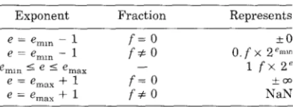
Table 2. IEEE 754 Special Values
Exponent Fraction Represents
~=~ nun –1 f=o *O
e = ‘ml. -1 f#o Ofx 2’mLn
e~,n 5 e 5 emax 1 fx2’
e=emay+l f:o
e=g ~ay + 1 f#o N%;
bit pattern represents a valid num-ber, the return value of square root must be some floating-point number. In the case of System/370 FORTRAN,
~ = 2 is returned. In IEEE
arith-metic, an NaN is returned in this
situation.
The IEEE standard specifies the fol-lowing special values (see Table 2): f O, denormalized numbers, + co and NaNs
(there is more than one NaN, as
ex-plained in the next section). These
special values are all encoded with exponents of either e~.X + 1 or e~,~ – 1 (it was already pointed out that O has an exponent of e~,. – 1).
2.2.1 NaNs
Traditionally, the computation of 0/0 or 4 – 1 has been treated as an unrecover-able error that causes a computation to halt. There are, however, examples for which it makes sense for a computation to continue in such a situation. Consider a subroutine that finds the zeros of a function f, say zero(f). Traditionally, zero finders require the user to input an interval [a, b] on which the function is defined and over which the zero finder will search. That is, the subroutine is called as zero(f, a, b). A more useful zero finder would not require the user to in-put this extra information. This more general zero finder is especially appropri-ate for calculators, where it is natural to key in a function and awkward to then have to specify the domain. It is easy, however, to see why most zero finders require a domain. The zero finder does its work by probing the function f at various values. If it probed for a value outside the domain of f, the code for f
Floating-Point Arithmetic 9 21
Table 3. Operations that Produce an NaN Operation NaN Produced by
+ W+(–w)
x Oxw
I
0/0, cO/03REM x REM O, m REM y fi(when x < O) \
might well compute 0/0 or ~, and
the computation would halt, unnecessar-ily aborting the zero finding process.
This problem can be avoided by intro-ducing a special value called NaN and specifying that the computation of
ex-pressions like 0/0 and ~ produce
NaN rather than halting. (A list of some of the situations that can cause a NaN is given in Table 3.) Then, when zero(f) probes outside the domain of f, the code for f will return NaN and the zero finder can continue. That is, zero(f) is not “punished” for making an incorrect guess. With this example in mind, it is easy to see what the result of combining a NaN with an ordinary floating-point number should be. Suppose the final statement off is return( – b + sqrt(d))/ (2* a). If d <0, then f should return a NaN. Since d <0, sqrt(d) is an NaN, and – b + sqrt(d) will be a NaN if the
sum of an NaN and any other number
is a NaN. Similarly, if one operand
of a division operation is an NaN,
the quotient should be a NaN. In
general, whenever a NaN participates
in a floating-point operation, the
result is another NaN.
Another approach to writing a zero solver that does not require the user to input a domain is to use signals. The zero finder could install a signal handler for floating-point exceptions. Then if f were evaluated outside its domain and raised an exception, control would be re-turned to the zero solver. The problem with this approach is that every lan-guage has a different method of handling signals (if it has a method at all), and so it has no hope of portability.
In IEEE 754, NaNs are represented as floating-point numbers with the
expo-nent e~~X + 1 and nonzero significands. Implementations are free to put system-dependent information into the signifi-cant. Thus, there is not a unique NaN but rather a whole family of NaNs. When an NaN and an ordinary floating-point number are combined, the result should be the same as the NaN operand. Thus, if the result of a long computation is an NaN, the system-dependent information in the significant will be the information generated when the first NaN in the computation was generated. Actually, there is a caveat to the last statement. If both operands are NaNs, the result will be one of those NaNs but it might not be the NaN that was generated first.
2.2.2 Infinity
Just as NaNs provide a way to continue a computation when expressions like 0/0 or ~ are encountered, infinities pro-vide a way to continue when an overflow occurs. This is much safer than simply returning to the largest representable number. As an example, consider
com-puting ~~, when b = 10, p = 3,
and e~~X = 98. If x = 3 x 1070 and
y = 4 X 1070, th en X2 will overflow and be replaced by 9.99 x 1098. Similarly yz and X2 + yz will each overflow in turn and be replaced by 9.99 x 1098. So the final result will be (9.99 x 1098)112 = 3.16 x 1049, which is drastically wrong. The correct answer is 5 x 1070. In IEEE arithmetic, the result of X2 is CO,as is
yz, X2 + yz, and -. SO the final
result is m, which is safer than
returning an ordinary floating-point number that is nowhere near the correct answer.”
The division of O by O results in an
NaN. A nonzero number divided by O,
however, returns infinity: 1/0 = ~, – 1/0 = – co. The reason for the distinc-tion is this: If f(x) -0 and g(x) + O as
llFine point: Although the default in IEEE arith-metic is to round overflowed numbers to ~, it is possible to change the default (see Section 2.3.2).
22 “ David Goldberg
x approaches some limit, then f( x)/g( x)
could have any value. For example,
when f’(x) = sin x and g(x) = x, then ~(x)/g(x) ~ 1 as x + O. But when ~(x)
=l– COSX, f(x)/g(x) ~ O. When
thinking of 0/0 as the limiting situation of a quotient of two very small numbers, 0/0 could represent anything. Thus, in the IEEE standard, 0/0 results in an NaN. But when c >0 and f(x) ~ c, g(x) ~ O, then ~(x)/g(*) ~ * m for any ana-lytic functions f and g. If g(x) <0 for small x, then f(x)/g(x) ~ – m; other-wise the limit is + m. So the IEEE stan-dard defines c/0 = & m as long as c # O. The sign of co depends on the signs of c and O in the usual way, so – 10/0 = – co
and –10/–0= +m. You can
distin-guish between getting m because of over-flow and getting m because of division by O by checking the status flags (which will be discussed in detail in Section 2.3.3). The overflow flag will be set in the first case, the division by O flag in the second.
The rule for determining the result of an operation that has infinity as an operand is simple: Replace infinity with a finite number x and take the limit as
x + m. Thus, 3/m = O, because
Iim ~+~3/x = O. Similarly 4 – co = – aI
and G = w. When the limit does not
exist, the result is an NaN, so m/co will be an NaN (Table 3 has additional exam-ples). This agrees with the reasoning used to conclude that 0/0 should be an NaN.
When a subexpression evaluates to a NaN, the value of the entire expression is also a NaN. In the case of & w, how-ever, the value of the expression might be an ordinary floating-point number be-cause of rules like I/m = O. Here is a practical example that makes use of the rules for infinity arithmetic. Consider computing the function x/( X2 + 1). This is a bad formula, because not only will it
overflow when x is larger than
fib’”” iz but infinity arithmetic will give the &rong answer because it will yield O rather than a number near 1/x. However, x/( X2 + 1) can be rewritten as 1/( x + x- l). This improved expression will not overflow prematurely and be-cause of infinity arithmetic will have the
correct value when x = O: 1/(0 + 0-1) = 1/(0 + CO)= l/CO = O. Without infinity arithmetic, the expression 1/( x + x-1) requires a test for x = O, which not only adds extra instructions but may also dis-rupt a pipeline. This example illustrates a general fact; namely, that infinity arithmetic often avoids the need for spe -cial case checking; however, formulas need to be carefully inspected to make sure they do not have spurious behavior at infinity [as x/(X2 + 1) did].
2.2.3 Slgnea Zero
Zero is represented by the exponent emm – 1 and a zero significant. Since the sign bit can take on two different values, there are two zeros, + O and – O. If a distinction were made when comparing -t O and – O, simple tests like if (x = O) would have unpredictable behavior, de-pending on the sign of x. Thus, the IEEE standard defines comparison so that
+0= –O rather than –O< +0.
Al-though it would be possible always to ignore the sign of zero, the IEEE stan-dard does not do so. When a multiplica-tion or division involves a signed zero, the usual sign rules apply in computing the sign of the answer. Thus, 3(+ O) = -t O and +0/– 3 = – O. If zero did not have a sign, the relation 1/(1 /x) = x would fail
to hold when x = *m. The reason is
that 1/– ~ and 1/+ ~ both result in O, and 1/0 results in + ~, the sign informa-tion having been lost. One way to restore the identity 1/(1 /x) = x is to have only one kind of’ infinity; however, that would result in the disastrous consequence of losing the sign of an overflowed quantity.
Another example of the use of signed zero concerns underflow and functions that have a discontinuity at zero such as log. In IEEE arithmetic, it is natural to define log O = – w and log x to be an NaN whe”n x <0. Suppose” x represents a small negative number that has under-flowed to zero. Thanks to signed zero, x will be negative so log can return an
NaN. If there were no signed zero,
however, the log function could not
Floating-Point Arithmetic “ 23
distinguish an underflowed negative number from O and would therefore have
to return – m. Another example of a
function with a discontinuity at zero is the signum function, which returns the sign of a number.
Probably the most interesting use of signed zero occurs in complex arithmetic. As an example, consider the equation
~ = ~/&. This is certainly true when z = O. If z = —1. the obvious
com-putation gives ~~ = ~ = i and
I/n= I/i = –i. Thus, ~#
1/W ! The problem can be traced to the fact that square root is multivalued, and there is no way to select the values so they are continuous in the entire com-plex plane. Square root is continuous, however, if a branch cut consisting of all negative real numbers is excluded from consideration. This leaves the problem of what to do for the negative real numbers, which are of the form – x + iO, where x > 0. Signed zero provides a perfect way to resolve this problem. Numbers of the form – x + i( + O) have a square root of
i&, and numbers of the form – x +
i( – O)on the other side of the branch cut have a square root with the other sign (– i ~). In fact, the natural formulas for computing ~ will give these results.
Let us return to ~ = l/fi. If z =
–1= –l+iO, then
1/2 = 1/(-1 + iO)
1(-1 -iO)
— —
(-1+ iO)(-1-iO)
= (-1 - iO)/(( -1)2 - 02) = –l+i(–0),
so ~= – 1+ i(–0) = –i, while
I/&= l/i = –i, Thus, IEEE arith-metic preserves this identity for all z. Some more sophisticated examples are given by Kahan [1987]. Although distin-guishing between + O and – O has advan-tages, it can occasionally be confusing. For example, signed zero destroys the relation x = y * I/x = l/y, which is
false when x = +0 and y = –O. The
IEEE committee decided, however, that the advantages of using signed zero out-weighed the disadvantages.
2.2.4 Denormalized Numbers
Consider normalized floating-point num-bers with O = 10, p = 3, and e~,. = –98. The numbers % = 6.87 x 10-97 and y = 6.81 x 10-97 appear to be perfectly ordi-nary floating-point numbers, which are more than a factor of 10 larger than the smallest floating-point number 1.00 x 10-98. They have a strange property, however: x 0 y = O even though x # y! The reason is that x – y = .06 x 10-97
—
—6.0 x 10- ‘g is too small to be repre-sented as a normalized number and so must be flushed to zero.
How important is it to preserve the property
X=yex–y=o? (lo)
It is very easy to imagine writing the code fragment if (x # y) then z = 1/ (x – y) and later having a program fail due to a spurious division by zero. Track-ing down bugs like this is frustrating and time consuming. On a more philo-sophical level, computer science text -books often point out that even though it is currently impractical to prove large programs correct, designing programs with the idea of proving them often re -suits in better code. For example, intro-ducing invariants is useful, even if they are not going to be used as part of a proof. Floating-point code is just like any other code: It helps to have provable facts on which to depend. For example, when analyzing formula (7), it will be helpful toknowthat x/2<y <2x*x Oy=x
— y (see Theorem 11). Similarly, know-ing that (10) is true makes writing reli-able floating-point code easier, If it is only true for most numbers, it cannot be used to prove anything.
The IEEE standard uses denormal-ized12 numbers, which guarantee (10), as
12They are called subnormal in 854, denormal in 754.
24 ● David Goldberg
I , , , , I t
1! I ,
, I I r I , t I , 1
I
~,,.+3
~
o P’-’ P-+’ P.=. +2 P-”+’
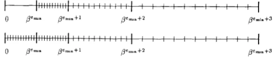
Figure 2. Flush to zero compared with gradual underflow.
well as other useful relations. They are the most controversial part of the stan-dard and probably accounted for the long delay in getting 754 approved. Most high-performance hardware that claims to be IEEE compatible does not support
denormalized numbers directly but
rather traps when consuming or produc-ing denormals, and leaves it to software to simulate the IEEE standard. 13 The idea behind denormalized numbers goes back to Goldberg [19671 and is simple. When the exponent is e~,., the signifi-cant does not have to be normalized. For example, when 13= 10, p = 3, and e~,.
—
— – 98, 1.00 x 10-98 is no longer the smallest floating-point number, because 0.98 x 10 -‘8 is also a floating-point number.
There is a small snag when P = 2 and a hidden bit is being used, since a num-ber with an exponent of e~,. will always have a significant greater than or equal to 1.0 because of the implicit leading bit. The solution is similar to that used to represent O and is summarized in Table 2. The exponent e~,. – 1 is used to rep-resent denormals. More formally, if the bits in the significant field are bl, bz~...~ bp–1 and the value of the expo-nent is e, then when e > e~,~ – 1, the number being represented is 1.bl bz . “ . b ~ x 2’, whereas when e = e~,~ – 1, t~e number being represented is 0.61 bz
. . . b ~_l x 2’+1. The + 1 in the exponent is needed because denormals have an ex-ponent of e~l., not e~,~ – 1.
13This M the cause of one of the most troublesome aspects of the #,andard. Programs that frequently underilow often run noticeably slower on hardware that uses software traps.
Recall the example O = 10, p = 3, e~,. —
— –98, x = 6.87 x 10-97, and y = 6.81 x 10-97
presented at the beginning of this section. With denormals, x – y does not flush to zero but is instead repre
-sented by the denormalized number
.6 X 10-98. This behavior is called gradual underflow. Itis easy to verify
that (10) always holds when using
gradual underflow.
Figure 2 illustrates denormalized
numbers. The top number line in the
figure shows normalized floating-point numbers. Notice the gap between O and the smallest normalized number 1.0 x ~em~. If the result of a floating-point cal-culation falls into this gulf, it is flushed to zero. The bottom number line shows what happens when denormals are added to the set of floating-point numbers. The “gulf’ is filled in; when the result of a calculation is less than 1.0 x ~’m~, it is represented by the nearest denormal.
When denormalized numbers are added
to the number line, the spacing between adjacent floating-point numbers varies in a regular way: Adjacent spacings are ei-ther the same length or differ by a factor of f3. Without denormals, the spacing abruptly changes from B ‘P+ lflem~ to ~em~, which is a factor of PP– 1, rather than the orderly change by a factor of ~, Because of this, many algorithms that can have large relative error for normalized num-bers close to the underflow threshold are well behaved in this range when gradual underflow is used.
Without gradual underflow, the simple expression x + y can have a very large relative error for normalized inputs, as was seen above for x = 6.87 x 10–97 and y = 6.81 x 10-97. L arge relative errors can happen even without cancellation, as