From Frequency to Meaning:
Vector Space Models of Semantics
Peter D. Turney [email protected]
National Research Council Canada Ottawa, Ontario, Canada, K1A 0R6
Patrick Pantel [email protected]
Yahoo! Labs
Sunnyvale, CA, 94089, USA
Abstract
Computers understand very little of the meaning of human language. This profoundly limits our ability to give instructions to computers, the ability of computers to explain their actions to us, and the ability of computers to analyse and process text. Vector space models (VSMs) of semantics are beginning to address these limits. This paper surveys the use of VSMs for semantic processing of text. We organize the literature on VSMs according to the structure of the matrix in a VSM. There are currently three broad classes of VSMs, based on term–document, word–context, and pair–pattern matrices, yielding three classes of applications. We survey a broad range of applications in these three categories and we take a detailed look at a specific open source project in each category. Our goal in this survey is to show the breadth of applications of VSMs for semantics, to provide a new perspective on VSMs for those who are already familiar with the area, and to provide pointers into the literature for those who are less familiar with the field.
1. Introduction
One of the biggest obstacles to making full use of the power of computers is that they currently understand very little of the meaning of human language. Recent progress in search engine technology is only scratching the surface of human language, and yet the impact on society and the economy is already immense. This hints at the transformative impact that deeper semantic technologies will have. Vector space models (VSMs), surveyed in this paper, are likely to be a part of these new semantic technologies.
In this paper, we use the termsemanticsin a general sense, as the meaning of a word, a phrase, a sentence, or any text in human language, and the study of such meaning. We are not concerned with narrower senses ofsemantics, such as thesemantic webor approaches to semantics based on formal logic. We present a survey of VSMs and their relation with the distributional hypothesis as an approach to representing some aspects of natural language semantics.
The VSM was developed for the SMART information retrieval system (Salton, 1971) by Gerard Salton and his colleagues (Salton, Wong, & Yang, 1975). SMART pioneered many of the concepts that are used in modern search engines (Manning, Raghavan, & Sch¨utze, 2008). The idea of the VSM is to represent each document in a collection as a point in a space (a vector in a vector space). Points that are close together in this space are semantically similar and points that are far apart are semantically distant. The user’s
query is represented as a point in the same space as the documents (the query is a pseudo-document). The documents are sorted in order of increasing distance (decreasing semantic similarity) from the query and then presented to the user.
The success of the VSM for information retrieval has inspired researchers to extend the VSM to other semantic tasks in natural language processing, with impressive results. For instance, Rapp (2003) used a vector-based representation of word meaning to achieve a score of 92.5% on multiple-choice synonym questions from the Test of English as a Foreign Language (TOEFL), whereas the average human score was 64.5%.1 Turney (2006) used a vector-based representation of semantic relations to attain a score of 56% on multiple-choice analogy questions from the SAT college entrance test, compared to an average human score of 57%.2
In this survey, we have organized past work with VSMs according to the type of matrix involved: term–document, word–context, and pair–pattern. We believe that the choice of a particular matrix type is more fundamental than other choices, such as the particular linguistic processing or mathematical processing. Although these three matrix types cover most of the work, there is no reason to believe that these three types exhaust the possibilities. We expect future work will introduce new types of matrices and higher-order tensors.3 1.1 Motivation for Vector Space Models of Semantics
VSMs have several attractive properties. VSMs extract knowledge automatically from a given corpus, thus they require much less labour than other approaches to semantics, such as hand-coded knowledge bases and ontologies. For example, the main resource used in Rapp’s (2003) VSM system for measuring word similarity is the British National Corpus (BNC),4whereas the main resource used in non-VSM systems for measuring word similarity (Hirst & St-Onge, 1998; Leacock & Chodrow, 1998; Jarmasz & Szpakowicz, 2003) is a lexicon, such as WordNet5 or Roget’s Thesaurus. Gathering a corpus for a new language
is generally much easier than building a lexicon, and building a lexicon often involves also gathering a corpus, such as SemCor for WordNet (Miller, Leacock, Tengi, & Bunker, 1993). VSMs perform well on tasks that involve measuring the similarity of meaning between words, phrases, and documents. Most search engines use VSMs to measure the similarity between a query and a document (Manning et al., 2008). The leading algorithms for mea-suring semantic relatedness use VSMs (Pantel & Lin, 2002a; Rapp, 2003; Turney, Littman, Bigham, & Shnayder, 2003). The leading algorithms for measuring the similarity of seman-tic relations also use VSMs (Lin & Pantel, 2001; Turney, 2006; Nakov & Hearst, 2008). (Section 2.4 discusses the differences between these types of similarity.)
We find VSMs especially interesting due to their relation with the distributional hy-pothesis and related hypotheses (see Section 2.7). The distributional hyhy-pothesis is that
1. Regarding the average score of 64.5% on the TOEFL questions, Landauer and Dumais (1997) note that, “Although we do not know how such a performance would compare, for example, with U.S. school children of a particular age, we have been told that the average score is adequate for admission to many universities.”
2. This is the average score for highschool students in their senior year, applying to US universities. For more discussion of this score, see Section 6.3 in Turney’s (2006) paper.
3. A vector is a first-order tensor and a matrix is a second-order tensor. See Section 2.5. 4. See http://www.natcorp.ox.ac.uk/.
words that occur in similar contexts tend to have similar meanings (Wittgenstein, 1953; Harris, 1954; Weaver, 1955; Firth, 1957; Deerwester, Dumais, Landauer, Furnas, & Harsh-man, 1990). Efforts to apply this abstract hypothesis to concrete algorithms for measuring the similarity of meaning often lead to vectors, matrices, and higher-order tensors. This intimate connection between the distributional hypothesis and VSMs is a strong motivation for taking a close look at VSMs.
Not all uses of vectors and matrices count as vector space models. For the purposes of this survey, we take it as a defining property of VSMs that the values of the elements in a VSM must be derived from event frequencies, such as the number of times that a given word appears in a given context (see Section 2.6). For example, often a lexicon or a knowledge base may be viewed as a graph, and a graph may be represented using an adjacency matrix, but this does not imply that a lexicon is a VSM, because, in general, the values of the elements in an adjacency matrix are not derived from event frequencies. This emphasis on event frequencies brings unity to the variety of VSMs and explicitly connects them to the distributional hypothesis; furthermore, it avoids triviality by excluding many possible matrix representations.
1.2 Vectors in AI and Cognitive Science
Vectors are common in AI and cognitive science; they were common before the VSM was introduced by Salton et al. (1975). The novelty of the VSM was to use frequencies in a corpus of text as a clue for discovering semantic information.
In machine learning, a typical problem is to learn to classify or cluster a set of items (i.e., examples, cases, individuals, entities) represented as feature vectors (Mitchell, 1997; Witten & Frank, 2005). In general, the features are not derived from event frequencies, although this is possible (see Section 4.6). For example, a machine learning algorithm can be applied to classifying or clustering documents (Sebastiani, 2002).
Collaborative filtering and recommender systems also use vectors (Resnick, Iacovou, Suchak, Bergstrom, & Riedl, 1994; Breese, Heckerman, & Kadie, 1998; Linden, Smith, & York, 2003). In a typical recommender system, we have a person-item matrix, in which the rows correspond to people (customers, consumers), the columns correspond to items (products, purchases), and the value of an element is the rating (poor, fair, excellent) that the person has given to the item. Many of the mathematical techniques that work well with term–document matrices (see Section 4) also work well with person-item matrices, but ratings are not derived from event frequencies.
In cognitive science, prototype theory often makes use of vectors. The basic idea of prototype theory is that some members of a category are more central than others (Rosch & Lloyd, 1978; Lakoff, 1987). For example, robin is a central (prototypical) member of the category bird, whereas penguin is more peripheral. Concepts have varying degrees of membership in categories (graded categorization). A natural way to formalize this is to represent concepts as vectors and categories as sets of vectors (Nosofsky, 1986; Smith, Osh-erson, Rips, & Keane, 1988). However, these vectors are usually based on numerical scores that are elicited by questioning human subjects; they are not based on event frequencies.
Another area of psychology that makes extensive use of vectors is psychometrics, which studies the measurement of psychological abilities and traits. The usual instrument for
measurement is a test or questionnaire, such as a personality test. The results of a test are typically represented as asubject-itemmatrix, in which the rows represent the subjects (people) in an experiment and the columns represent the items (questions) in the test (questionnaire). The value of an element in the matrix is the answer that the corresponding subject gave for the corresponding item. Many techniques for vector analysis, such as factor analysis (Spearman, 1904), were pioneered in psychometrics.
In cognitive science, Latent Semantic Analysis (LSA) (Deerwester et al., 1990; Lan-dauer & Dumais, 1997), Hyperspace Analogue to Language (HAL) (Lund, Burgess, & Atchley, 1995; Lund & Burgess, 1996), and related research (Landauer, McNamara, Den-nis, & Kintsch, 2007) is entirely within the scope of VSMs, as defined above, since this research uses vector space models in which the values of the elements are derived from event frequencies, such as the number of times that a given word appears in a given con-text. Cognitive scientists have argued that there are empirical and theoretical reasons for believing that VSMs, such as LSA and HAL, are plausible models of some aspects of hu-man cognition (Landauer et al., 2007). In AI, computational linguistics, and information retrieval, such plausibility is not essential, but it may be seen as a sign that VSMs are a promising area for further research.
1.3 Motivation for This Survey
This paper is a survey of vector space models of semantics. There is currently no com-prehensive, up-to-date survey of this field. As we show in the survey, vector space models are a highly successful approach to semantics, with a wide range of potential and actual applications. There has been much recent growth in research in this area.
This paper should be of interest to all AI researchers who work with natural language, especially researchers who are interested in semantics. The survey will serve as a general introduction to this area and it will provide a framework – a unified perspective – for organizing the diverse literature on the topic. It should encourage new research in the area, by pointing out open problems and areas for further exploration.
This survey makes the following contributions:
New framework: We provide a new framework for organizing the literature: term– document, word–context, and pair–pattern matrices (see Section 2). This framework shows the importance of the structure of the matrix (the choice of rows and columns) in deter-mining the potential applications and may inspire researchers to explore new structures (different kinds of rows and columns, or higher-order tensors instead of matrices).
New developments: We draw attention to pair–pattern matrices. The use of pair– pattern matrices is relatively new and deserves more study. These matrices address some criticisms that have been directed at word–context matrices, regarding lack of sensitivity to word order.
Breadth of approaches and applications: There is no existing survey that shows the breadth of potential and actual applications of VSMs for semantics. Existing summaries omit pair–pattern matrices (Landauer et al., 2007).
Focus on NLP and CL: Our focus in this survey is on systems that perform practical tasks in natural language processing and computational linguistics. Existing overviews focus on cognitive psychology (Landauer et al., 2007).
Success stories: We draw attention to the fact that VSMs are arguably the most successful approach to semantics, so far.
1.4 Intended Readership
Our goal in writing this paper has been to survey the state of the art in vector space models of semantics, to introduce the topic to those who are new to the area, and to give a new perspective to those who are already familiar with the area.
We assume our reader has a basic understanding of vectors, matrices, and linear algebra, such as one might acquire from an introductory undergraduate course in linear algebra, or from a text book (Golub & Van Loan, 1996). The basic concepts of vectors and matrices are more important here than the mathematical details. Widdows (2004) gives a gentle introduction to vectors from the perspective of semantics.
We also assume our reader has some familiarity with computational linguistics or infor-mation retrieval. Manning et al. (2008) provide a good introduction to inforinfor-mation retrieval. For computational linguistics, we recommend Manning and Sch¨utze’s (1999) text.
If our reader is familiar with linear algebra and computational linguistics, this survey should present no barriers to understanding. Beyond this background, it is not necessary to be familiar with VSMs as they are used in information retrieval, natural language pro-cessing, and computational linguistics. However, if the reader would like to do some further background reading, we recommend Landauer et al.’s (2007) collection.
1.5 Highlights and Outline
This article is structured as follows. Section 2 explains our framework for organizing the literature on VSMs according to the type of matrix involved: term–document, word–context, and pair–pattern. In this section, we present an overview of VSMs, without getting into the details of how a matrix can be generated from a corpus of raw text.
After the high-level framework is in place, Sections 3 and 4 examine the steps involved in generating a matrix. Section 3 discusses linguistic processing and Section 4 reviews mathematical processing. This is the order in which a corpus would be processed in most VSM systems (first linguistic processing, then mathematical processing).
When VSMs are used for semantics, the input to the model is usually plain text. Some VSMs work directly with the raw text, but most first apply some linguistic processing to the text, such as stemming, part-of-speech tagging, word sense tagging, or parsing. Section 3 looks at some of these linguistic tools for semantic VSMs.
In a simple VSM, such as a simple term–document VSM, the value of an element in a document vector is the number of times that the corresponding word occurs in the given document, but most VSMs apply some mathematical processing to the raw frequency values. Section 4 presents the main mathematical operations: weighting the elements, smoothing the matrix, and comparing the vectors. This section also describes optimization strategies for comparing the vectors, such as distributed sparse matrix multiplication and randomized techniques.
By the end of Section 4, the reader will have a general view of the concepts involved in vector space models of semantics. We then take a detailed look at three VSM systems in Section 5. As a representative of term–document VSMs, we present the Lucene information
retrieval library.6 For word–context VSMs, we explore the Semantic Vectors package, which builds on Lucene.7 As the representative of pair–pattern VSMs, we review the Latent Relational Analysis module in the S-Space package, which also builds on Lucene.8 The source code for all three of these systems is available under open source licensing.
We turn to a broad survey of applications for semantic VSMs in Section 6. This sec-tion also serves as a short historical view of research with semantic VSMs, beginning with information retrieval in Section 6.1. Our purpose here is to give the reader an idea of the breadth of applications for VSMs and also to provide pointers into the literature, if the reader wishes to examine any of these applications in detail.
In a term–document matrix, rows correspond to terms and columns correspond to doc-uments (Section 6.1). A document provides a context for understanding the term. If we generalize the idea of documents to chunks of text of arbitrary size (phrases, sentences, paragraphs, chapters, books, collections), the result is the word–context matrix, which in-cludes the term–document matrix as a special case. Section 6.2 discusses applications for word–context matrices. Section 6.3 considerspair–patternmatrices, in which the rows cor-respond to pairs of terms and the columns corcor-respond to the patterns in which the pairs occur.
In Section 7, we discuss alternatives to VSMs for semantics. Section 8 considers the future of VSMs, raising some questions about their power and their limitations. We conclude in Section 9.
2. Vector Space Models of Semantics
The theme that unites the various forms of VSMs that we discuss in this paper can be stated as thestatistical semantics hypothesis: statistical patterns of human word usage can be used to figure out what people mean.9 This general hypothesis underlies several more specific hypotheses, such as the bag of words hypothesis, the distributional hypothesis, the
extended distributional hypothesis, and thelatent relation hypothesis, discussed below. 2.1 Similarity of Documents: The Term–Document Matrix
In this paper, we use the following notational conventions: Matrices are denoted by bold capital letters,A. Vectors are denoted by bold lowercase letters, b. Scalars are represented by lowercase italic letters,c.
If we have a large collection of documents, and hence a large number of document vectors, it is convenient to organize the vectors into a matrix. The row vectors of the matrix correspond to terms (usually terms are words, but we will discuss some other possibilities)
6. See http://lucene.apache.org/java/docs/. 7. See http://code.google.com/p/semanticvectors/.
8. See http://code.google.com/p/airhead-research/wiki/LatentRelationalAnalysis.
9. This phrase was taken from the Faculty Profile of George Furnas at the University of Michigan, http://www.si.umich.edu/people/faculty-detail.htm?sid=41. The full quote is, “Statistical Semantics – Studies of how the statistical patterns of human word usage can be used to figure out what people mean, at least to a level sufficient for information access.” The term statistical semanticsappeared in the work of Furnas, Landauer, Gomez, and Dumais (1983), but it was not defined there.
and the column vectors correspond to documents (web pages, for example). This kind of matrix is called a term–documentmatrix.
In mathematics, a bag (also called a multiset) is like a set, except that duplicates are allowed. For example,{a, a, b, c, c, c}is a bag containinga,b, andc. Order does not matter in bags and sets; the bags{a, a, b, c, c, c}and{c, a, c, b, a, c}are equivalent. We can represent the bag{a, a, b, c, c, c} with the vector x=h2,1,3i, by stipulating that the first element of xis the frequency ofain the bag, the second element is the frequency of bin the bag, and the third element is the frequency of c. A set of bags can be represented as a matrixX, in which each columnx:j corresponds to a bag, each rowxi: corresponds to a unique member,
and an elementxij is the frequency of thei-th member in thej-th bag.
In a term–document matrix, a document vector represents the corresponding document as a bag of words. In information retrieval, the bag of words hypothesis is that we can estimate the relevance of documents to a query by representing the documents and the query as bags of words. That is, the frequencies of words in a document tend to indicate the relevance of the document to a query. The bag of words hypothesis is the basis for applying the VSM to information retrieval (Salton et al., 1975). The hypothesis expresses the belief that a column vector in a term–document matrix captures (to some degree) an aspect of the meaning of the corresponding document; what the document is about.
Let Xbe a term–document matrix. Suppose our document collection contains n docu-ments andm unique terms. The matrixXwill then havem rows (one row for each unique term in the vocabulary) andncolumns (one column for each document). Letwi be thei-th term in the vocabulary and let dj be the j-th document in the collection. Thei-th row in X is the row vectorxi: and the j-th column in Xis the column vector x:j. The row vector xi:containsnelements, one element for each document, and the column vectorx:j contains m elements, one element for each term. SupposeX is a simple matrix of frequencies. The elementxij inX is the frequency of the i-th term wi in thej-th document dj.
In general, the value of most of the elements in X will be zero (the matrix is sparse), since most documents will use only a small fraction of the whole vocabulary. If we randomly choose a term wi and a documentdj, it’s likely that wi does not occur anywhere indj, and therefore xij equals 0.
The pattern of numbers in xi: is a kind of signature of the i-th term wi; likewise, the pattern of numbers in x:j is a signature of the j-th document dj. That is, the pattern of numbers tells us, to some degree, what the term or document is about.
The vectorx:j may seem to be a rather crude representation of the documentdj. It tells us how frequently the words appear in the document, but the sequential order of the words is lost. The vector does not attempt to capture the structure in the phrases, sentences, paragraphs, and chapters of the document. However, in spite of this crudeness, search engines work surprisingly well; vectors seem to capture an important aspect of semantics.
The VSM of Salton et al. (1975) was arguably the first practical, useful algorithm for extracting semantic information from word usage. An intuitive justification for the term– document matrix is that the topic of a document will probabilistically influence the author’s choice of words when writing the document.10 If two documents have similar topics, then the two corresponding column vectors will tend to have similar patterns of numbers.
10. Newer generative models, such as Latent Dirichlet Allocation (LDA) (Blei, Ng, & Jordan, 2003), directly model this intuition. See Sections 4.3 and 7.
2.2 Similarity of Words: The Word–Context Matrix
Salton et al. (1975) focused on measuring document similarity, treating a query to a search engine as a pseudo-document. The relevance of a document to a query is given by the similarity of their vectors. Deerwester et al. (1990) observed that we can shift the focus to measuring word similarity, instead of document similarity, by looking at row vectors in the term–document matrix, instead of column vectors.
Deerwester et al. (1990) were inspired by the term–document matrix of Salton et al. (1975), but a document is not necessarily the optimal length of text for measuring word similarity. In general, we may have a word–context matrix, in which the context is given by words, phrases, sentences, paragraphs, chapters, documents, or more exotic possibilities, such as sequences of characters or patterns.
The distributional hypothesis in linguistics is that words that occur in similar contexts tend to have similar meanings (Harris, 1954). This hypothesis is the justification for ap-plying the VSM to measuring word similarity. A word may be represented by a vector in which the elements are derived from the occurrences of the word in various contexts, such as windows of words (Lund & Burgess, 1996), grammatical dependencies (Lin, 1998; Pad´o & Lapata, 2007), and richer contexts consisting of dependency links and selectional preferences on the argument positions (Erk & Pad´o, 2008); see Sahlgren’s (2006) thesis for a comprehensive study of various contexts. Similar row vectors in the word–context matrix indicate similar word meanings.
The idea that word usage can reveal semantics was implicit in some of the things that Wittgenstein (1953) said about language-games and family resemblance. Wittgenstein was primarily interested in the physical activities that form the context of word usage (e.g., the wordbrick, spoken in the context of the physical activity of building a house), but the main context for a word is often other words.11
Weaver (1955) argued that word sense disambiguation for machine translation should be based on the co-occurrence frequency of the context words near a given target word (the word that we want to disambiguate). Firth (1957, p. 11) said, “You shall know a word by the company it keeps.” Deerwester et al. (1990) showed how the intuitions of Wittgen-stein (1953), Harris (1954), Weaver, and Firth could be used in a practical algorithm. 2.3 Similarity of Relations: The Pair–Pattern Matrix
In a pair–pattern matrix, row vectors correspond to pairs of words, such as mason:stone
and carpenter:wood, and column vectors correspond to the patterns in which the pairs co-occur, such as “X cuts Y” and “X works with Y”. Lin and Pantel (2001) introduced the pair–pattern matrix for the purpose of measuring the semantic similarity of patterns; that is, the similarity of column vectors. Given a pattern such as “X solves Y”, their algorithm was able to find similar patterns, such as “Y is solved by X”, “Y is resolved in X”, and “X resolves Y”.
Lin and Pantel (2001) proposed the extended distributional hypothesis, that patterns that co-occur with similar pairs tend to have similar meanings. The patterns “X solvesY”
11. Wittgenstein’s intuition might be better captured by a matrix that combines words with other modalities, such as images (Monay & Gatica-Perez, 2003). If the values of the elements are derived from event frequencies, we would include this as a VSM approach to semantics.
and “Y is solved byX” tend to co-occur with similarX:Y pairs, which suggests that these patterns have similar meanings. Pattern similarity can be used to infer that one sentence is a paraphrase of another (Lin & Pantel, 2001).
Turney et al. (2003) introduced the use of the pair–pattern matrix for measuring the semantic similarity of relations between word pairs; that is, the similarity of row vectors. For example, the pairs mason:stone, carpenter:wood, potter:clay, and glassblower:glass
share the semantic relation artisan:material. In each case, the first member of the pair is an artisan who makes artifacts from the material that is the second member of the pair. The pairs tend to co-occur in similar patterns, such as “theX used the Y to” and “theX
shaped theY into”.
The latent relation hypothesis is that pairs of words that co-occur in similar patterns tend to have similar semantic relations (Turney, 2008a). Word pairs with similar row vectors in a pair–pattern matrix tend to have similar semantic relations. This is the inverse of the extended distributional hypothesis, that patterns with similar column vectors in the pair–pattern matrix tend to have similar meanings.
2.4 Similarities
Pair–pattern matrices are suited to measuring the similarity of semantic relations between pairs of words; that is, relational similarity. In contrast, word–context matrices are suited to measuring attributional similarity. The distinction between attributional and relational similarity has been explored in depth by Gentner (1983).
The attributional similarity between two wordsaand b, sima(a, b)∈ <, depends on the
degree of correspondence between the properties ofaandb. The more correspondence there is, the greater their attributional similarity. The relational similarity between two pairsof words a:b and c:d, simr(a:b, c:d) ∈ <, depends on the degree of correspondence between
the relations ofa:band c:d. The more correspondence there is, the greater their relational similarity. For example, dogand wolf have a relatively high degree of attributional similar-ity, whereas dog:bark and cat:meow have a relatively high degree of relational similarity (Turney, 2006).
It is tempting to suppose that relational similarity can be reduced to attributional similarity. For example, mason and carpenter are similar words and stone and wood are similar words; therefore, perhaps it follows that mason:stone and carpenter:wood have similar relations. Perhaps simr(a:b, c:d) can be reduced to sima(a, c) + sima(b, d). However, mason, carpenter, potter, and glassblower are similar words (they are all artisans), as are
wood, clay, stone, and glass (they are all materials used by artisans), but we cannot infer from this thatmason:glassandcarpenter:clayhave similar relations. Turney (2006, 2008a) presented experimental evidence that relational similarity does not reduce to attributional similarity.
The term semantic relatednessin computational linguistics (Budanitsky & Hirst, 2001) corresponds to attributional similarity in cognitive science (Gentner, 1983). Two words are semantically related if they have any kind of semantic relation (Budanitsky & Hirst, 2001); they are semantically related to the degree that they share attributes (Turney, 2006). Examples are synonyms (bank and trust company), meronyms (car and wheel), antonyms (hot andcold), and words that are functionally related or frequently associated (pencil and
paper). We might not usually think that antonyms are similar, but antonyms have a high degree of attributional similarity (hot and cold are kinds of temperature, black and white are kinds of colour, loud and quiet are kinds of sound). We prefer the term attributional similarityto the termsemantic relatedness, becauseattributional similarity emphasizes the contrast with relational similarity, whereas semantic relatedness could be confused with
relational similarity.
In computational linguistics, the termsemantic similarityis applied to words that share a hypernym (car and bicycle are semantically similar, because they share the hypernym
vehicle) (Resnik, 1995). Semantic similarity is a specific type of attributional similarity. We prefer the term taxonomical similarity to the term semantic similarity, because the term
semantic similarity is misleading. Intuitively, both attributional and relational similarity involve meaning, so both deserve to be called semantic similarity.
Words are semantically associated if they tend to co-occur frequently (e.g., bee and
honey) (Chiarello, Burgess, Richards, & Pollock, 1990). Words may be taxonomically simi-lar and semantically associated (doctorand nurse), taxonomically similar but not semanti-cally associated (horseandplatypus), semantically associated but not taxonomically similar (cradleandbaby), or neither semantically associated nor taxonomically similar (calculusand
candy).
Sch¨utze and Pedersen (1993) defined two ways that words can be distributed in a cor-pus of text: If two words tend to be neighbours of each other, then they are syntagmatic associates. If two words have similar neighbours, then they areparadigmatic parallels. Syn-tagmatic associates are often different parts of speech, whereas paradigmatic parallels are usually the same part of speech. Syntagmatic associates tend to be semantically associ-ated (beeandhoney are often neighbours); paradigmatic parallels tend to be taxonomically similar (doctor and nursehave similar neighbours).
2.5 Other Semantic VSMs
The possibilities are not exhausted by term–document, word–context, and pair–pattern matrices. We might want to consider triple–pattern matrices, for measuring the semantic similarity between word triples. Whereas a pair–pattern matrix might have a row mason:
stone and a column “X works with Y”, a triple–pattern matrix could have a row mason:
stone:masonry and a column “X uses Y to build Z”. However, n-tuples of words grow increasingly rare as n increases. For example, phrases that contain mason, stone, and
masonrytogether are less frequent than phrases that containmasonandstone together. A triple–pattern matrix will be much more sparse than a pair–pattern matrix (ceteris paribus). The quantity of text that we need, in order to have enough numbers to make our matrices useful, grows rapidly as n increases. It may be better to break n-tuples into pairs. For example,a:b:ccould be decomposed intoa:b,a:c, andb:c(Turney, 2008a). The similarity of two triples,a:b:candd:e:f, could be estimated by the similarity of their corresponding pairs. A relatively dense pair–pattern matrix could serve as a surrogate for a relatively sparse triple–pattern matrix.
We may also go beyond matrices. The generalization of a matrix is a tensor (Kolda & Bader, 2009; Acar & Yener, 2009). A scalar (a single number) is zeroth-order tensor, a vector is first-order tensor, and a matrix is a second-order tensor. A tensor of order three or
higher is called a higher-order tensor. Chew, Bader, Kolda, and Abdelali (2007) use a term– document–language third-order tensor for multilingual information retrieval. Turney (2007) uses a word–word–pattern tensor to measure similarity of words. Van de Cruys (2009) uses a verb–subject–object tensor to learn selectional preferences of verbs.
In Turney’s (2007) tensor, for example, rows correspond to words from the TOEFL multiple-choice synonym questions, columns correspond to words from Basic English (Og-den, 1930),12 and tubescorrespond to patterns that join rows and columns (hence we have a word–word–pattern third-order tensor). A given word from the TOEFL questions is rep-resented by the corresponding word–pattern matrix slice in the tensor. The elements in this slice correspond to all the patterns that relate the given TOEFL word to any word in Basic English. The similarity of two TOEFL words is calculated by comparing the two corresponding matrix slices. The algorithm achieves 83.8% on the TOEFL questions. 2.6 Types and Tokens
Atokenis a single instance of a symbol, whereas atypeis a general class of tokens (Manning et al., 2008). Consider the following example (from Samuel Beckett):
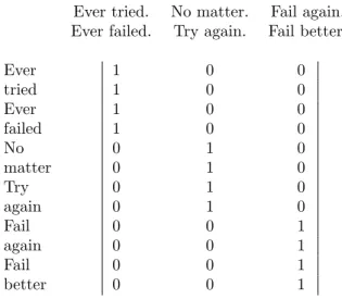
Ever tried. Ever failed. No matter. Try again. Fail again. Fail better.
There are two tokens of the type Ever, two tokens of the type again, and two tokens of the type Fail. Let’s say that each line in this example is a document, so we have three documents of two sentences each. We can represent this example with a token–document matrix or a type–document matrix. The token–document matrix has twelve rows, one for each token, and three columns, one for each line (Figure 1). The type–document matrix has nine rows, one for each type, and three columns (Figure 2).
A row vector for a token has binary values: an element is 1 if the given token appears in the given document and 0 otherwise. A row vector for a type has integer values: an element is the frequency of the given type in the given document. These vectors are related, in that a type vector is the sum of the corresponding token vectors. For example, the row vector for the typeEver is the sum of the two token vectors for the two tokens ofEver.
In applications dealing with polysemy, one approach uses vectors that represent word tokens (Sch¨utze, 1998; Agirre & Edmonds, 2006) and another uses vectors that represent word types (Pantel & Lin, 2002a). Typical word sense disambiguation (WSD) algorithms deal with word tokens (instances of words in specific contexts) rather than word types. We mention both approaches to polysemy in Section 6, due to their similarity and close relationship, although a defining characteristic of the VSM is that it is concerned with frequencies (see Section 1.1), and frequency is a property of types, not tokens.
12. Basic English is a highly reduced subset of English, designed to be easy for people to learn. The words of Basic English are listed at http://ogden.basic-english.org/.
Ever tried. No matter. Fail again. Ever failed. Try again. Fail better.
Ever 1 0 0
tried 1 0 0
Ever 1 0 0
failed 1 0 0
No 0 1 0
matter 0 1 0
Try 0 1 0
again 0 1 0
Fail 0 0 1
again 0 0 1
Fail 0 0 1
better 0 0 1
Figure 1: The token–document matrix. Rows are tokens and columns are documents.
Ever tried. No matter. Fail again. Ever failed. Try again. Fail better.
Ever 2 0 0
tried 1 0 0
failed 1 0 0
No 0 1 0
matter 0 1 0
Try 0 1 0
again 0 1 1
Fail 0 0 2
better 0 0 1
2.7 Hypotheses
We have mentioned five hypotheses in this section. Here we repeat these hypotheses and then interpret them in terms of vectors. For each hypothesis, we cite work that explicitly states something like the hypothesis or implicitly assumes something like the hypothesis.
Statistical semantics hypothesis: Statistical patterns of human word usage can be used to figure out what people mean (Weaver, 1955; Furnas et al., 1983). – If units of text have similar vectors in a text frequency matrix,13then they tend to have similar meanings.
(We take this to be a general hypothesis that subsumes the four more specific hypotheses that follow.)
Bag of words hypothesis: The frequencies of words in a document tend to indicate the relevance of the document to a query (Salton et al., 1975). – If documents and pseudo-documents (queries) have similar column vectors in a term–document matrix, then they tend to have similar meanings.
Distributional hypothesis: Words that occur in similar contexts tend to have similar meanings (Harris, 1954; Firth, 1957; Deerwester et al., 1990). – If words have similar row vectors in a word–context matrix, then they tend to have similar meanings.
Extended distributional hypothesis: Patterns that co-occur with similar pairs tend to have similar meanings (Lin & Pantel, 2001). – If patterns have similar column vectors in a pair–pattern matrix, then they tend to express similar semantic relations.
Latent relation hypothesis: Pairs of words that co-occur in similar patterns tend to have similar semantic relations (Turney et al., 2003). – If word pairs have similar row vectors in a pair–pattern matrix, then they tend to have similar semantic relations.
We have not yet explained what it means to say that vectors are similar. We discuss this in Section 4.4.
3. Linguistic Processing for Vector Space Models
We will assume that our raw data is a large corpus of natural language text. Before we generate a term–document, word–context, or pair–pattern matrix, it can be useful to apply some linguistic processing to the raw text. The types of processing that are used can be grouped into three classes. First, we need totokenizethe raw text; that is, we need to decide what constitutes aterm and how to extract terms from raw text. Second, we may want to
normalize the raw text, to convert superficially different strings of characters to the same form (e.g., car, Car, cars, and Cars could all be normalized to car). Third, we may want toannotatethe raw text, to mark identical strings of characters as being different (e.g.,fly
as a verb could be annotated asfly/VBand flyas a noun could be annotated as fly/NN). Grefenstette (1994) presents a good study of linguistic processing for word–context VSMs. He uses a similar three-step decomposition of linguistic processing: tokenization, surface syntactic analysis, and syntactic attribute extraction.
13. Bytext frequency matrix, we mean any matrix or higher-order tensor in which the values of the elements are derived from the frequencies of pieces of text in the context of other pieces of text in some collection of text. A text frequency matrix is intended to be a general structure, which includes term–document, word–context, and pair–pattern matrices as special cases.
3.1 Tokenization
Tokenization of English seems simple at first glance: words are separated by spaces. This assumption is approximately true for English, and it may work sufficiently well for a basic VSM, but a more advanced VSM requires a more sophisticated approach to tokenization.
An accurate English tokenizer must know how to handle punctuation (e.g.,don’t,Jane’s,
and/or), hyphenation (e.g.,state-of-the-artversusstate of the art), and recognize multi-word terms (e.g., Barack Obama and ice hockey) (Manning et al., 2008). We may also wish to ignore stop words, high-frequency words with relatively low information content, such as function words (e.g., of,the, and) and pronouns (e.g., them, who, that). A popular list of stop words is the set of 571 common words included in the source code for the SMART system (Salton, 1971).14
In some languages (e.g., Chinese), words are not separated by spaces. A basic VSM can break the text into character unigrams or bigrams. A more sophisticated approach is to match the input text against entries in a lexicon, but the matching often does not determine a unique tokenization (Sproat & Emerson, 2003). Furthermore, native speakers often disagree about the correct segmentation. Highly accurate tokenization is a challenging task for most human languages.
3.2 Normalization
The motivation for normalization is the observation that many different strings of charac-ters often convey essentially identical meanings. Given that we want to get at the meaning that underlies the words, it seems reasonable to normalize superficial variations by con-verting them to the same form. The most common types of normalization are case folding (converting all words to lower case) and stemming (reducing inflected words to their stem or root form).
Case folding is easy in English, but can be problematic in some languages. In French, accents are optional for uppercase, and it may be difficult to restore missing accents when converting the words to lowercase. Some words cannot be distinguished without accents; for example,PECHE could be either pˆeche(meaning fishingorpeach) or p´ech´e(meaningsin). Even in English, case folding can cause problems, because case sometimes has semantic significance. For example, SMART is an information retrieval system, whereas smart is a common adjective; Bushmay be a surname, whereas bush is a kind of plant.
Morphology is the study of the internal structure of words. Often a word is composed of a stem (root) with added affixes (inflections), such as plural forms and past tenses (e.g.,
trappedis composed of the stemtrap and the affix-ed). Stemming, a kind of morphological analysis, is the process of reducing inflected words to their stems. In English, affixes are simpler and more regular than in many other languages, and stemming algorithms based on heuristics (rules of thumb) work relatively well (Lovins, 1968; Porter, 1980; Minnen, Carroll, & Pearce, 2001). In anagglutinative language (e.g., Inuktitut), many concepts are combined into a single word, using various prefixes, infixes, and suffixes, and morphological analysis is complicated. A single word in an agglutinative language may correspond to a sentence of half a dozen words in English (Johnson & Martin, 2003).
The performance of an information retrieval system is often measured by precision and recall (Manning et al., 2008). The precision of a system is an estimate of the conditional probability that a document is truly relevant to a query, if the system says it is relevant. Therecallof a system is an estimate of the conditional probability that the system will say that a document is relevant to a query, if it truly is relevant.
In general, normalization increases recall and reduces precision (Kraaij & Pohlmann, 1996). This is natural, given the nature of normalization. When we remove superficial variations that we believe are irrelevant to meaning, we make it easier to recognize similar-ities; we find more similar things, and so recall increases. But sometimes these superficial variations have semantic significance; ignoring the variations causes errors, and so precision decreases. Normalization can also have a positive effect on precision in cases where variant tokens are infrequent and smoothing the variations gives more reliable statistics.
If we have a small corpus, we may not be able to afford to be overly selective, and it may be best to aggressively normalize the text, to increase recall. If we have a very large corpus, precision may be more important, and we might not want any normalization. Hull (1996) gives a good analysis of normalization for information retrieval.
3.3 Annotation
Annotation is the inverse of normalization. Just as different strings of characters may have the same meaning, it also happens that identical strings of characters may have different meanings, depending on the context. Common forms of annotation include part-of-speech tagging (marking words according to their parts of speech), word sense tagging (marking ambiguous words according to their intended meanings), and parsing (analyzing the gram-matical structure of sentences and marking the words in the sentences according to their grammatical roles) (Manning & Sch¨utze, 1999).
Since annotation is the inverse of normalization, we expect it to decrease recall and increase precision. For example, by tagging program as a noun or a verb, we may be able to selectively search for documents that are about the act of computer programming (verb) instead of documents that discuss particular computer programs (noun); hence we can increase precision. However, a document about computer programs (noun) may have something useful to say about the act of computer programming (verb), even if the document never uses the verb form ofprogram; hence we may decrease recall.
Large gains in IR performance have recently been reported as a result of query an-notation with syntactic and semantic information. Syntactic anan-notation includes query segmentation (Tan & Peng, 2008) and part of speech tagging (Barr, Jones, & Regelson, 2008). Examples of semantic annotation are disambiguating abbreviations in queries (Wei, Peng, & Dumoulin, 2008) and finding query keyword associations (Lavrenko & Croft, 2001; Cao, Nie, & Bai, 2005).
Annotation is also useful for measuring the semantic similarity of words and concepts (word–context matrices). For example, Pantel and Lin (2002a) presented an algorithm that can discover word senses by clustering row vectors in a word–context matrix, using contextual information derived from parsing.
4. Mathematical Processing for Vector Space Models
After the text has been tokenized and (optionally) normalized and annotated, the first step is to generate a matrix of frequencies. Second, we may want to adjust the weights of the elements in the matrix, because common words will have high frequencies, yet they are less informative than rare words. Third, we may want to smooth the matrix, to reduce the amount of random noise and to fill in some of the zero elements in a sparse matrix. Fourth, there are many different ways to measure the similarity of two vectors.
Lowe (2001) gives a good summary of mathematical processing for word–context VSMs. He decomposes VSM construction into a similar four-step process: calculate the frequencies, transform the raw frequency counts, smooth the space (dimensionality reduction), then calculate the similarities.
4.1 Building the Frequency Matrix
An element in a frequency matrix corresponds to an event: a certain item (term, word, word pair) occurred in a certain situation (document, context, pattern) a certain number of times (frequency). At an abstract level, building a frequency matrix is a simple matter of counting events. In practice, it can be complicated when the corpus is large.
A typical approach to building a frequency matrix involves two steps. First, scan se-quentially through the corpus, recording events and their frequencies in a hash table, a database, or a search engine index. Second, use the resulting data structure to generate the frequency matrix, with a sparse matrix representation (Gilbert, Moler, & Schreiber, 1992). 4.2 Weighting the Elements
The idea of weighting is to give more weight to surprising events and less weight to expected events. The hypothesis is that surprising events, if shared by two vectors, are more dis-criminative of the similarity between the vectors than less surprising events. For example, in measuring the semantic similarity between the wordsmouseand rat, the contexts dissect
andexterminateare more discriminative of their similarity than the contextshaveandlike. In information theory, a surprising event has higher information content than an expected event (Shannon, 1948). The most popular way to formalize this idea for term–document matrices is the tf-idf (term frequency × inverse document frequency) family of weighting functions (Sp¨arck Jones, 1972). An element gets a high weight when the corresponding term is frequent in the corresponding document (i.e., tf is high), but the term is rare in other documents in the corpus (i.e., df is low, and thus idf is high). Salton and Buckley (1988) defined a large family of tf-idf weighting functions and evaluated them on information re-trieval tasks, demonstrating that tf-idf weighting can yield significant improvements over raw frequency.
Another kind of weighting, often combined with tf-idf weighting, is length normalization (Singhal, Salton, Mitra, & Buckley, 1996). In information retrieval, if document length is ignored, search engines tend to have a bias in favour of longer documents. Length normalization corrects for this bias.
Term weighting may also be used to correct for correlated terms. For example, the terms hostageand hostages tend to be correlated, yet we may not want to normalize them
to the same term (as in Section 3.2), because they have slightly different meanings. As an alternative to normalizing them, we may reduce their weights when they co-occur in a document (Church, 1995).
Feature selection may be viewed as a form of weighting, in which some terms get a weight of zero and hence can be removed from the matrix. Forman (2003) provides a good study of feature selection methods for text classification.
An alternative to tf-idf is Pointwise Mutual Information (PMI) (Church & Hanks, 1989; Turney, 2001), which works well for both word–context matrices (Pantel & Lin, 2002a) and term–document matrices (Pantel & Lin, 2002b). A variation of PMI is Positive PMI (PPMI), in which all PMI values that are less than zero are replaced with zero (Niwa & Nitta, 1994). Bullinaria and Levy (2007) demonstrated that PPMI performs better than a wide variety of other weighting approaches when measuring semantic similarity with word– context matrices. Turney (2008a) applied PPMI to pair–pattern matrices. We will give the formal definition of PPMI here, as an example of an effective weighting function.
Let Fbe a word–context frequency matrix withnr rows and nccolumns. The i-th row in F is the row vector fi: and the j-th column in F is the column vector f:j. The row fi:
corresponds to a word wi and the columnf:j corresponds to a contextcj. The value of the element fij is the number of times that wi occurs in the context cj. Let X be the matrix that results when PPMI is applied to F. The new matrix Xhas the same number of rows and columns as the raw frequency matrix F. The value of an element xij in X is defined as follows:
pij =
fij
Pnr i=1
Pnc j=1fij
(1)
pi∗ =
Pnc j=1fij
Pnr i=1
Pnc j=1fij
(2)
p∗j =
Pnr i=1fij Pnr
i=1 Pnc
j=1fij
(3) pmiij = log
pij pi∗p∗j
(4)
xij =
pmiij if pmiij >0
0 otherwise (5)
In this definition,pij is the estimated probability that the wordwi occurs in the context cj,pi∗ is the estimated probability of the wordwi, and p∗j is the estimated probability of the contextcj. Ifwi andcj are statistically independent, thenpi∗p∗j =pij (by the definition of independence), and thus pmiij is zero (since log(1) = 0). The productpi∗p∗j is what we would expect forpij ifwi occurs incj by pure random chance. On the other hand, if there is an interesting semantic relation betweenwi andcj, then we should expectpij to be larger than it would be if wi and cj were indepedent; hence we should find that pij > pi∗p∗j, and thus pmiij is positive. This follows from the distributional hypothesis (see Section 2). If the word wi is unrelated to the context cj, we may find that pmiij is negative. PPMI is designed to give a high value toxij when there is an interesting semantic relation between
wi and cj; otherwise,xij should have a value of zero, indicating that the occurrence of wi incj is uninformative.
A well-known problem of PMI is that it is biased towards infrequent events. Consider the case wherewi and cj are statistically dependent (i.e., they have maximum association). Thenpij =pi∗ =p∗j. Hence (4) becomes log (1/pi∗) and PMI increases as the probability of wordwidecreases. Several discounting factors have been proposed to alleviate this problem. An example follows (Pantel & Lin, 2002a):
δij = fij fij + 1
· min (
Pnr k=1fkj,
Pnc k=1fik) min (Pnr
k=1fkj, Pnc
k=1fik) + 1
(6)
newpmiij =δij·pmiij (7)
Another way to deal with infrequent events is Laplace smoothing of the probability estimates,pij,pi∗, andp∗j (Turney & Littman, 2003). A constant positive value is added to the raw frequencies before calculating the probabilities; eachfij is replaced withfij+k, for somek >0. The larger the constant, the greater the smoothing effect. Laplace smoothing pushes the pmiij values towards zero. The magnitude of the push (the difference between pmiij with and without Laplace smoothing) depends on the raw frequency fij. If the frequency is large, the push is small; if the frequency is small, the push is large. Thus Laplace smoothing reduces the bias of PMI towards infrequent events.
4.3 Smoothing the Matrix
The simplest way to improve information retrieval performance is to limit the number of vector components. Keeping only components representing the most frequently occurring content words is such a way; however, common words, such as the and have, carry little semantic discrimination power. Simple component smoothing heuristics, based on the prop-erties of the weighting schemes presented in Section 4.2, have been shown to both maintain semantic discrimination power and improve the performance of similarity computations.
Computing the similarity between all pairs of vectors, described in Section 4.4, is a computationally intensive task. However, only vectors that share a non-zero coordinate must be compared (i.e., two vectors that do not share a coordinate are dissimilar). Very frequent context words, such as the wordthe, unfortunately result in most vectors matching a non-zero coordinate. Such words are precisely the contexts that have little semantic discrimination power. Consider the pointwise mutual information weighting described in Section 4.2. Highly weighted dimensions co-occur frequently with only very few words and are by definition highly discriminating contexts (i.e., they have very high association with the words with which they co-occur). By keeping only the context-word dimensions with a PMI above a conservative threshold and setting the others to zero, Lin (1998) showed that the number of comparisons needed to compare vectors greatly decreases while losing little precision in the similarity score between the top-200 most similar words of every word. While smoothing the matrix, one computes a reverse index on the non-zero coordinates. Then, to compare the similarity between a word’s context vector and all other words’ context vectors, only those vectors found to match a non-zero component in the reverse index must be compared. Section 4.5 proposes further optimizations along these lines.
Deerwester et al. (1990) found an elegant way to improve similarity measurements with a mathematical operation on the term–document matrix,X, based on linear algebra. The op-eration is truncated Singular Value Decomposition (SVD), also called thin SVD. Deerwester et al. briefly mentioned that truncated SVD can be applied to both document similarity and word similarity, but their focus was document similarity. Landauer and Dumais (1997) applied truncated SVD to word similarity, achieving human-level scores on multiple-choice synonym questions from the Test of English as a Foreign Language (TOEFL). Truncated SVD applied to document similarity is called Latent Semantic Indexing (LSI), but it is called Latent Semantic Analysis (LSA) when applied to word similarity.
There are several ways of thinking about how truncated SVD works. We will first present the math behind truncated SVD and then describe four ways of looking at it: latent meaning, noise reduction, high-order co-occurrence, and sparsity reduction.
SVD decomposes X into the product of three matricesUΣVT, where U and V are in column orthonormal form (i.e., the columns are orthogonal and have unit length, UTU= VTV=I) and Σ is a diagonal matrix of singular values (Golub & Van Loan, 1996). If X is of rank r, thenΣis also of rank r. LetΣk, wherek < r, be the diagonal matrix formed from the topksingular values, and letUkandVkbe the matrices produced by selecting the corresponding columns fromU and V. The matrix UkΣkVkT is the matrix of rankk that best approximates the original matrixX, in the sense that it minimizes the approximation errors. That is, Xˆ =UkΣkVTk minimizes kXˆ −XkF over all matrices Xˆ of rank k, where
k. . .kF denotes the Frobenius norm (Golub & Van Loan, 1996).
Latent meaning: Deerwester et al. (1990) and Landauer and Dumais (1997) describe truncated SVD as a method for discovering latent meaning. Suppose we have a word– context matrix X. The truncated SVD, Xˆ = UkΣkVTk, creates a low-dimensional linear mapping between row space (words) and column space (contexts). This low-dimensional mapping captures the latent (hidden) meaning in the words and the contexts. Limiting the number of latent dimensions (k < r) forces a greater correspondence between words and contexts. This forced correspondence between words and contexts improves the similarity measurement.
Noise reduction: Rapp (2003) describes truncated SVD as a noise reduction technique. We may think of the matrixXˆ =UkΣkVTk as a smoothed version of the original matrixX. The matrix Uk maps the row space (the space spanned by the rows of X) into a smaller k-dimensional space and the matrix Vk maps the column space (the space spanned by the columns of X) into the same k-dimensional space. The diagonal matrix Σk specifies the weights in this reduced k-dimensional space. The singular values in Σ are ranked in descending order of the amount of variation in X that they fit. If we think of the matrix X as being composed of a mixture of signal and noise, with more signal than noise, then UkΣkVTk mostly captures the variation inXthat is due to the signal, whereas the remaining vectors in UΣVT are mostly fitting the variation in Xthat is due to the noise.
High-order co-occurrence: Landauer and Dumais (1997) also describe truncated SVD as a method for discovering high-order co-occurrence. Direct co-occurrence (first-order co-occurrence) is when two words appear in identical contexts. Indirect co-occurrence (high-order co-occurrence) is when two words appear in similar contexts. Similarity of contexts may be defined recursively in terms of lower-order co-occurrence. Lemaire and Denhi`ere (2006) demonstrate that truncated SVD can discover high-order co-occurrence.
Sparsity reduction: In general, the matrixX is very sparse (mostly zeroes), but the truncated SVD,Xˆ =UkΣkVTk, is dense. Sparsity may be viewed as a problem of insufficient data: with more text, the matrixX would have fewer zeroes, and the VSM would perform better on the chosen task. From this perspective, truncated SVD is a way of simulating the missing text, compensating for the lack of data (Vozalis & Margaritis, 2003).
These different ways of viewing truncated SVD are compatible with each other; it is possible for all of these perspectives to be correct. Future work is likely to provide more views of SVD and perhaps a unifying view.
A good C implementation of SVD for large sparse matrices is Rohde’s SVDLIBC.15 Another approach is Brand’s (2006) incremental truncated SVD algorithm.16 Yet another approach is Gorrell’s (2006) Hebbian algorithm for incremental truncated SVD. Brand’s and Gorrell’s algorithms both introduce interesting new ways of handling missing values, instead of treating them as zero values.
For higher-order tensors, there are operations that are analogous to truncated SVD, such as parallel factor analysis (PARAFAC) (Harshman, 1970), canonical decomposition (CANDECOMP) (Carroll & Chang, 1970) (equivalent to PARAFAC but discovered inde-pendently), and Tucker decomposition (Tucker, 1966). For an overview of tensor decompo-sitions, see the surveys of Kolda and Bader (2009) or Acar and Yener (2009). Turney (2007) gives an empirical evaluation of how well four different Tucker decomposition algorithms scale up for large sparse third-order tensors. A low-RAM algorithm, Multislice Projection, for large sparse tensors is presented and evaluated.17
Since the work of Deerwester et al. (1990), subsequent research has discovered many alternative matrix smoothing processes, such as Nonnegative Matrix Factorization (NMF) (Lee & Seung, 1999), Probabilistic Latent Semantic Indexing (PLSI) (Hofmann, 1999), Iter-ative Scaling (IS) (Ando, 2000), Kernel Principal Components Analysis (KPCA) (Scholkopf, Smola, & Muller, 1997), Latent Dirichlet Allocation (LDA) (Blei et al., 2003), and Discrete Component Analysis (DCA) (Buntine & Jakulin, 2006).
The four perspectives on truncated SVD, presented above, apply equally well to all of these more recent matrix smoothing algorithms. These newer smoothing algorithms tend to be more computationally intensive than truncated SVD, but they attempt to model word frequencies better than SVD. Truncated SVD implicitly assumes that the elements in X have a Gaussian distribution. Minimizing the the Frobenius norm kXˆ −XkF will minimize the noise, if the noise has a Gaussian distribution. However, it is known that word frequencies do not have Gaussian distributions. More recent algorithms are based on more realistic models of the distribution for word frequencies.18
4.4 Comparing the Vectors
The most popular way to measure the similarity of two frequency vectors (raw or weighted) is to take their cosine. Letxand y be two vectors, each withn elements.
15. SVDLIBC is available at http://tedlab.mit.edu/∼dr/svdlibc/.
16. MATLAB source code is available at http://web.mit.edu/∼wingated/www/resources.html.
17. MATLAB source code is available at http://www.apperceptual.com/multislice/.
18. In our experience, pmiijappears to be approximately Gaussian, which may explain why PMI works well with truncated SVD, but then PPMI is puzzling, because it is less Gaussian than PMI, yet it apparently yields better semantic models than PMI.
x=hx1, x2, . . . , xni (8) y=hy1, y2, . . . , yni (9) The cosine of the angleθ betweenx andy can be calculated as follows:
cos(x,y) =
Pn
i=1xi·yi q
Pn
i=1x2i ·
Pn
i=1y2i
(10)
= √ x·y
x·x·√y·y (11)
= x
kxk·
y
kyk (12)
In other words, the cosine of the angle between two vectors is the inner product of the vectors, after they have been normalized to unit length. If x and y are frequency vectors for words, a frequent word will have a long vector and a rare word will have a short vector, yet the words might be synonyms. Cosine captures the idea that the length of the vectors is irrelevant; the important thing is the angle between the vectors.
The cosine ranges from −1 when the vectors point in opposite directions (θ is 180 degrees) to +1 when they point in the same direction (θ is 0 degrees). When the vectors are orthogonal (θ is 90 degrees), the cosine is zero. With raw frequency vectors, which necessarily cannot have negative elements, the cosine cannot be negative, but weighting and smoothing often introduce negative elements. PPMI weighting does not yield negative elements, but truncated SVD can generate negative elements, even when the input matrix has no negative values.
A measure of distance between vectors can easily be converted to a measure of similarity by inversion (13) or subtraction (14).
sim(x,y) = 1/dist(x,y) (13)
sim(x,y) = 1−dist(x,y) (14)
Many similarity measures have been proposed in both IR (Jones & Furnas, 1987) and lexical semantics circles (Lin, 1998; Dagan, Lee, & Pereira, 1999; Lee, 1999; Weeds, Weir, & McCarthy, 2004). It is commonly said in IR that, properly normalized, the difference in retrieval performance using different measures is insignificant (van Rijsbergen, 1979). Often the vectors are normalized in some way (e.g., unit length or unit probability) before applying any similarity measure.
Popular geometric measures of vector distance include Euclidean distance and Manhat-tan disManhat-tance. DisManhat-tance measures from information theory include Hellinger, Bhattacharya, and Kullback-Leibler. Bullinaria and Levy (2007) compared these five distance measures and the cosine similarity measure on four different tasks involving word similarity. Overall, the best measure was cosine. Other popular measures are the Dice and Jaccard coefficients (Manning et al., 2008).
Lee (1999) proposed that, for finding word similarities, measures that focused more on overlapping coordinates and less on the importance of negative features (i.e., coordinates where one word has a nonzero value and the other has a zero value) appear to perform better. In Lee’s experiments, the Jaccard, Jensen-Shannon, and L1 measures seemed to perform best. Weeds et al. (2004) studied the linguistic and statistical properties of the similar words returned by various similarity measures and found that the measures can be grouped into three classes:
1. high-frequency sensitive measures (cosine, Jensen-Shannon,α-skew, recall), 2. low-frequency sensitive measures (precision), and
3. similar-frequency sensitive methods (Jaccard, Jaccard+MI, Lin, harmonic mean). Given a word w0, if we use a high-frequency sensitive measure to score other words wi according to their similarity withw0, higher frequency words will tend to get higher scores
than lower frequency words. If we use a low-frequency sensitive measure, there will be a bias towards lower frequency words. Similar-frequency sensitive methods prefer a wordwi that has approximately the same frequency as w0. In one experiment on determining the
compositionality of collocations, high-frequency sensitive measures outperformed the other classes (Weeds et al., 2004). We believe that determining the most appropriate similarity measure is inherently dependent on the similarity task, the sparsity of the statistics, the frequency distribution of the elements being compared, and the smoothing method applied to the matrix.
4.5 Efficient Comparisons
Computing the similarity between all rows (or columns) in a large matrix is a non-trivial problem, with a worst case cubic running timeO(n2
rnc), wherenris the number of rows and nc is the number of columns (i.e., the dimensionality of the feature space). Optimizations and parallelization are often necessary.
4.5.1 Sparse-Matrix Multiplication
One optimization strategy is a generalized sparse-matrix multiplication approach (Sarawagi & Kirpal, 2004), which is based on the observation that a scalar product of two vectors depends only on the coordinates for which both vectors have nonzero values. Further, we observe that most commonly used similarity measures for vectorsx and y, such as cosine, overlap, and Dice, can be decomposed into three values: one depending only on the nonzero values ofx, another depending only on the nonzero values ofy, and the third depending on the nonzero coordinates shared both byxand y. More formally, commonly used similarity scores, sim(x,y), can be expressed as follows:
sim(x,y) =f0(Pni=1f1(xi, yi), f2(x), f3(y)) (15)
For example, the cosine measure, cos(x,y), defined in (10), can be expressed in this model as follows:
cos(x,y) =f0(Pni=1f1(xi, yi), f2(x), f3(y)) (16) f0(a, b, c) =
a
b·c (17)
f1(a, b) =a·b (18)
f2(a) =f3(a) = q
Pn
i=1a2i (19)
Let X be a matrix for which we want to compute the pairwise similarity, sim(x,y), between all rows or all columns x and y. Efficient computation of the similarity matrix S can be achieved by leveraging the fact that sim(x,y) is determined solely by the nonzero coordinates shared by x and y (i.e., f1(0, xi) = f1(xi,0) = 0 for any xi) and that most of the vectors are very sparse. In this case, calculating f1(xi, yi) is only required when both vectors have a shared nonzero coordinate, significantly reducing the cost of computation. Determining which vectors share a nonzero coodinate can easily be achieved by first building an inverted index for the coordinates. During indexing, we can also precomputef2(x) and f3(y) without changing the algorithm complexity. Then, for each vector x we retrieve in
constant time, from the index, each vectory that shares a nonzero coordinate with x and we apply f1(xi, yi) on the shared coordinates i. The computational cost of this algorithm isP
iNi2 whereNi is the number of vectors that have a nonzeroi-th coordinate. Its worst case time complexity is O(ncv) wheren is the number of vectors to be compared, cis the maximum number of nonzero coordinates of any vector, and v is the number of vectors that have a nonzeroi-th coordinate whereiis the coordinate which is nonzero for the most vectors. In other words, the algorithm is efficient only when the density of the coordinates is low. In our own experiments of computing the semantic similarity between all pairs of words in a large web crawl, we observed near linear average running time complexity inn. The computational cost can be reduced further by leveraging the element weighting techniques described in Section 4.2. By setting to zero all coordinates that have a low PPMI, PMI or tf-idf score, the coordinate density is dramatically reduced at the cost of losing little discriminative power. In this vein, Bayardo, Ma, and Srikant (2007) described a strategy that omits the coordinates with the highest number of nonzero values. Their algorithm gives a significant advantage only when we are interested in finding solely the similarity between highly similar vectors.
4.5.2 Distributed Implementation using MapReduce
The algorithm described in Section 4.5.1 assumes that the matrix X can fit into memory, which for large X may be impossible. Also, as each element of X is processed indepen-dently, running parallel processes for non-intersecting subsets of X makes the processing faster. Elsayed, Lin, and Oard (2008) proposed a MapReduce implementation deployed us-ing Hadoop, an open-source software package implementus-ing the MapReduce framework and distributed file system.19 Hadoop has been shown to scale to several thousands of machines, allowing users to write simple code, and to seamlessly manage the sophisticated parallel ex-ecution of the code. Dean and Ghemawat (2008) provide a good primer on MapReduce programming.