Single top production at the LHC:
the Effective
W
Approximation
∗D. Espriu† and J. Manzano‡
Departament d’Estructura i Constituents de la Mat`eria and IFAE,
Universitat de Barcelona, Diagonal, 647, E-08028 Barcelona
Abstract
We study the mechanism of single top production at the LHC, analyzing the sensitivity of different observables to the magnitude of the effective left and right couplings. The study is carried out in the framework of the so-called effective W approximation, where the virtualW is treated as a parton. The validity of this approximation in the present case is analyzed in detail by comparing it to an exact calculation. We comment on several issues related to top polarization since the observables relevant to distinguish between left and right effective couplings involve the measurement of the spin of the top. This can be achieved only indirectly measuring the angular distribution of top decay products. The effectiveW approximation is probably not well suited for this subtle analysis, but it remains a useful tool for a total cross section analysis.
UB-ECM-PF 01/09 August 2001
∗Contribution presented in the XXIX International Meeting on Fundamental Physics, Sitges, February
2001. Dedicated to F.J.Yndur´ain on his 60th birthday.
1
Introduction
It is quite conceivable that the Standard Model should be considered as an effective theory valid only at low energies (. 1 TeV ). In particular, since the Higgs particle has not been observed yet (the current bound on the Standard Model Higgs is at 113.5 GeV [1]), it makes sense to consider as an alternative to the minimal Standard Model an effective theory without any physical light scalar fields. Alternatively, it may well be that the Higgs particle, or, as a matter of fact, any other scalars, which abound in extensions of the minimal Standard Model, are much heavier than the weak scale, granting an expansion in inverse powers of such heavy masses. How heavy must the Higgs particle —or the scale associated to new physics, for that matter— be for such an expansion to be useful? In practice, 300 or 400 GeV are sufficient for the expansion to be useful at the MZ scale, as detailed calculations[2] show, and this is
expected to scale appropriately with the energy. In a process like the one we shall discuss in this paper, where the individual energies involved are peaked in the 200 - 400 region, the effective lagrangian techniques should be appropriate provided that the relevant scale is in the 1 TeV region. While admittedly this is not the scenario favoured by the comparison with the electroweak data[3], it cannot be properly excluded until a (relatively) light elementary Higgs is found.
If Nature has decided that no new light degrees of freedom exist in the vicinity of the weak scale, the proper way to deal with processes where the individual energies of all particles involved is well below the 1 TeV region involves the use of an effective lagrangian. In this effective lagrangian, only the light (respect to the energies of the process) degrees of freedom are kept, while the information about the heavier degrees of freedom is contained in an infinite set of effective operators of increasing dimensionality, compatible with the electroweak and strong symmetries SU(3)c ×SU(2)L×U(1)Y. The coefficients of these operators would
parametrize different choices of new physics beyond the Standard Model. In this framework [4] one can describe the low energy physics of theories exhibiting the pattern of symmetry breaking SU(2)L×U(1)Y → U(1)em. Both global and gauge symmetries are non-linearly
realized and the effective theory is non-renormalizable (the Higgs field, which is absent here, is a necessary ingredient both for the linear realization and renormalizability of the minimal Standard Model). The additional operators serve thus a dual purpose; on the one hand they encode low-energy effects of the so-far unexplored high-energy scales. On the other hand, these operators are necessary as counterterms to absorb ultraviolet divergences generated by quantum corrections from the lower dimensional (universal) terms.
In this work we are concerned about the new features that physics beyond the Standard Model may introduce in the production of single top quarks through W-gluon fusion at
the LHC. We are interested only in the leading non-universal (i.e. not appearing in the standard model at tree level) effective operators in the low energy expansion. In the present context these correspond to those operators of dimension four, which were first classified by Appelquist et al. [5]. These operators are characteristic of strongly coupled theories (i.e. of theories without an elementary Higgs or a very heavy one) and require a non-linear realization of the gauge symmetry. Therefore they are absent in the minimal Standard Model and in modifications thereof containing only light fields. When one particularizes to theW
interactions, for instance by going to the unitary gauge, these operators induce effective fermion-gauge boson couplings.
However, radiative corrections induce form factors in the vertices too. Assuming a smooth dependence in the external momenta these form factors can be expanded and at leading order in the derivative expansion they just induce effective fermion-gauge boson effective couplings. Obviously any deviation from the values of these couplings with respect to the values predicted by the minimal Standard Model would indicate the presence of new physics in the matter sector. To what extent can thus a machine like the LHC set direct bounds on these couplings, in particular those involving the top?
2
Top Production at the LHC
Let us now briefly review the mechanisms of top production. At the LHC energy (14 TeV) the dominant mechanism for creating tops is gluon-gluon fusion. This is a purely QCD process, its total cross-section is 800 pb[6]. It is obvious that tops will be copiously produced at the LHC and that a lot can be learned by a detailed analysis of their decays, for instance. We note, however, that this mechanism of production has nothing to do with the electroweak sector and thus is not the most adequate for our purposes. In fact, since colour symmetry, like electromagnetism, is unbroken, the form factor is unchanged at the lowest order in the derivative expansion and new physics cannot possibly affect this effective coupling at the order we are working [7]. In addition, we shall not be interested here in top decay, but rather in how new physics can affect the way top (or anti-top) are produced at the LHC. For these reasons, the dominant mechanism of top production at the LHC is not interesting at all for our purposes, and for us it will just be a background to worry about.
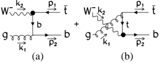
At tree level, electroweak physics enters the game through single top production. (For a recent review see e.g. [8].) At LHC energies the (by far) dominant electroweak subpro-cess contributing to single top production is given by a gluon (g) coming from one proton and a positively charged W+ coming from the other (this process is also called t-channel production[9, 10]). This process is depicted in diagrams (a) and (b) of Fig.1. The total cross
(a) (b)
Figure 1: Feynman diagrams contributing to the single top production subprocess
(a) (b)
Figure 2: Feynman diagrams contributing to the single anti-top production subprocess
section for this process at the LHC is 250 pb, to be compared to 50 pb for the associated production1 with aW+ boson and a b-quark extracted from the sea of the proton, and the 10 pb corresponding to quark-quark fusion (s-channel production). For a detailed discussion see [10]. For comparison, at the Tevatron (2 GeV) the cross section for W-gluon fusion is 2.5 pb, so the production of tops through this particular subprocess is really copious at the LHC. Monte Carlo simulations including the analysis of the top decay products indicate that this process can be analyzed in detail at the LHC and traditionally has been regarded as the most important one for our purposes.
In a proton-proton collision a bottom-anti-top pair is also produced, through the subpro-cesses (a) and (b) of Fig.2. However, these subprosubpro-cesses are suppressed roughly by a factor of two (see Fig.4) because the proton has much lesser probability of emitting a W− than emitting a W+, and at any rate qualitative results are very similar to those corresponding to the subprocess of Fig.1, from where the cross sections can be easily derived doing the appropriate changes.
Thus, even if subdominant, single top production through an electroweak vertex is not negligible at all; more than one third of all tops or anti-tops that will be produced at the LHC will be created through this mechanism. Furthermore, this mechanism has rather distinctive kinematics, as we shall see in this work. Indeed, single top production, being dominated by the exchange of a massless (by comparison to the energies involved) particle in thetchannel, is strongly peaked in the forward direction, with a characteristic angular distribution (see
1the difference between the two processes is purely kinematic; see section 5. The above values correspond
below).
Several analysis of top production exist in the literature. A (surely incomplete) list of the references we have used is given in [8, 9, 10] and [11, 12]. The second group of references is mostly concerned with the issue of the top polarization. Indeed, since the top decays shortly after production, much before strong effects can set in, the decaying products (abquark and a W, which, in turn, decays into e.g. a charged lepton and a neutrino) carry information about the spin of the top. In particular, if the top is in a pure state of spin (and hence being as= 1/2 fermion its polarization vector points in the top rest frame in a particular direction in space), the decaying lepton has an angular distribution peaked in the direction where the top polarization vector is pointing to.
So far the issue as to what extend LHC can set bounds on the top-bottom effective cou-plings has not been analyzed in much detail in the literature. The contribution from operators of dimension five to top production via longitudinal vector boson fusion was estimated some time ago in [13], although the study was by no means complete. It should be mentioned that
t,¯t pair production through this mechanism is very much masked by the dominant mecha-nism of gluon-gluon fusion, while single top production, throughW Z fusion, is expected to be quite suppressed compared to the mechanism presented in this paper, the reason being that both vertices are electroweak in the process discussed in [13], and that operators of dimension five are expected to be suppressed, at least at moderate energies, such as the ones that in practice count at LHC, by some large mass scale. The effects due to anomalous couplings introduced through operators of dimension six have been recently analyzed in [14]. All the contributions from higher dimensional operators are in realistic models expected to be small and far beyond the sensitivity of LHC. For these reasons we concentrate only on dimension four operators. In practice this means bounds on the left and right top effective couplings (see also [15]).
The potential for single top production for measuring the CKM matrix element Vtb, and
hence the top-bottom effective left coupling has certainly been previously studied (see e.g. [9], [10] and our recent work [16]), but drawing firm conclusions requires a good knowledge of the total normalization of the cross-section, something which is very influenced by issues on which a good theoretical control is problematic, such as the QCD scale. Next to leading calculations such as the ones presented in [17, 18] for the total cross section are mandatory but results still leave an uncertainty at the 5% level. Nothing is known on bounds on the right effective couplings. On the other hand, it is clear that this is a very urgent issue. The only noticeable discrepancy of the whole of the LEP results when compared to the minimal Standard Model lies in the bottom effective couplings (actually on the right coupling). Our main motivation for this work is to partly fill in this gap. This looks feasible with machines
like the LHC which are efficient top factories.
3
Effective Couplings
It is sometimes stated that gauge invariance prevents the presence of dimension four operators other than the ones already existing in the Standard Model, thus forcing the contribution of new physics to be suppressed by powers. This is not so when the symmetry is non-linearly realized The complete set of dimension four effective operators which may contribute to the top effective couplings is [5, 19]
L14 = iδ1¯fγµU(DµU)†Lf,
L24 = iδ2¯fγµU†(DµU)Rf,
L34 = iδ3¯fγµ(DµU)τ3U†Lf +h.c.,
L44 = iδ4¯fγµU τ3U†(DµU)τ3U†Lf,
L54 = iδ5¯fγµτ3U†(DµU)Rf +h.c.,
L6
4 = iδ6¯fγµτ3U†(DµU)τ3Rf,
L7
4 = iδ7¯fγµU τ3U†DµLLf +h.c.,
where L = 1−2γ5, R= 1+2γ5 are the left and right projectors. The matrix-valued field U(x) is an SU(2) matrix containing the three Goldstone bosons associated to the spontaneous breaking of the symmetry. The covariant derivatives appearing in the above operators are
DµU = ∂µU +ig
τ
2·WµU −ig
0Uτ3
2 Bµ,
DµLf =
∂µ+ig
τ
2·Wµ+ig
01
6Bµ+igs
λ
2·Gµ
f,
DµRf =
∂µ+i
g0
2
τ3+ 1 3
Bµ+igs
λ
2·Gµ
f,
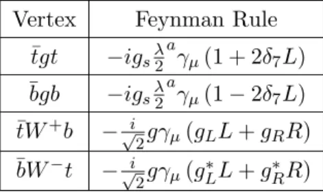
Finally f is a weak doublet of matter fields ((t, b) in our case). Generation mixing has been neglected. The above operators contribute to the different gauge boson-fermion-fermion vertices as indicated in table 1.
In addition, the operator L74 also contributes to the quark self energies Σu(p) = −26pδ7L,
Σd(p) = +26pδ7L, (1)
and to the counterterms required to guarantee the on-shell renormalization conditions [19]
δZdL= 2δ7, δZuL=−2δ7, δZdR= 0, δZuR= 0, δmd=−δ
Vertex Feynman Rule ¯
tgt −igsλ2 a
γµ(1 + 2δ7L)
¯bgb −igsλ 2 a
γµ(1−2δ7L)
¯
tW+b −√i
2gγµ(gLL+gRR)
¯
bW−t −√i
2gγµ(g∗LL+gR∗R)
Table 1: Feynman rules for the vertices appearing in the subprocesses of Figs.(1) and (2).
but when we take into account all these contributions,δ7 vanish from the observables in the present case. It should be noted, however, that the internal quark line in the diagrams in Figs.(1) and (2) are never on-shell and the use of the equations of motion to eliminate L74, is a priori not justified. The net effect of the electroweak effective lagrangian in the charged current sector can thus be summarized, to the order we have considered, in the effective couplings gLand gR.
gL= 1 +δgL= 1−(δ1+δ4) gR=δgR=δ2−δ6. (2)
Just for completeness, we list the effective couplings appropriate to the neutral sector
gfV = If3 1−2s2W +δ1−δ4−δ2−δ6−δ3−δ5−1
3s
2 W,
gAf = If3(1 +δ1−δ4+δ2+δ6)−δ3−δ5,
relevant for theZ →ff¯vertex [19].
At present not much is known from direct measurements for thet→b effective coupling. This is perhaps best evidenced by the fact that the current experimental results for the (left-handed) Vtb matrix element give [20]
|Vtb|2
|Vtd|2+|Vts|2+|Vtb|2
= 0.94+0−0..3124. (3) It should be emphasized that these are the ‘measured’ or ‘effective’ values of the CKM matrix elements, and that they do not necessarily correspond, even in the Standard Model, to the entries of a unitary matrix on account of the presence of radiative corrections, even though these deviations with respect to unitary are expected to be small unless new physics is present. At the Tevatron, it is said, the left-handed couplings are expected to be eventually measured with a 5% accuracy [21], but as mentioned above this depends on absolute scale normalizations which are hard to pin down, even after a full two-loop QCD calculation.
As far as experimental bounds for the right handed effective couplings is concerned no direct relevant bounds exist, the more stringent ones are indirect and come from the mea-surements on theb→sγ decay at CLEO [22]. Due to amt/mb enhancement of the chirality
flipping contribution, a particular combination of mixing angles andκCCR can be found. The authors of [23] reach the conclusion that|Re(κCCR )| ≤0.4×10⁻². However, considering κCCR
as a matrix in generation space, this bound only constraints thetb element. Other effective couplings involving the top remain virtually unrestricted from the data. Nonetheless the previous bound on the right-handed coupling is a very stringent one. It is fairly clear that an hadron machine such as the LHC will never be able to compete with such a precision. Yet, the measurement would be a direct one, not through loop corrections. Equally important is that it will yield information on the tsand td elements too, by just replacing the quark exchanged in thet-channel in Fig.1 (b).
4
The effective
W
approximation
The calculations presented in this work are carried out in the framework of the so-called effec-tive W approximation that is the translation to the present case of the familiar Weizs¨ acker-William[24] approximation for photons.
Known to be accurate at high energies (see e.g. [25] for a discussion on errors and improvements) and very convenient, this approach is caculationally simple and has all the attractive physical interpretation of the parton model. One certainly would expect that the approximation, even for W’s, is sufficiently good at LHC energies, where it has been amply used in the context ofW W,W ZorW γscattering. (See e.g. [26] for a very recent application and references.) We shall later discuss in more detail to what extent these expectations are fulfilled.
In this work the production of polarized tops is considered. As we shall see this is abso-lutely necessary if one wishes to set bounds on the right-handed effective couplings. In doing so we have found results which are somewhat at variance with the recent work reported in [11]. One of the conclusions of our work is that the differences are, to a large extent, due to the use of different kinematical cuts rather than being attributable to the effectiveW approx-imation itself. In spite of this, the effective W approximation has undoubtedly shortcomings which we shall review in detail in the coming pages by comparing their predictions to an exact calculation [16].
In order to calculate the cross section of the process pp→ t¯b we have used the CTEQ4 structure functions [27] to determine the probability of extracting a parton with a given fraction of momenta from the proton. Theu and d-type partons then radiate a W− or W+
boson, respectively.
In the effective W approximation theseW bosons (both longitudinal and transverse) are treated as partons from the proton, carrying a fraction of the quark momentum and thus of
the momentum of the proton. TheW parton distribution function is, roughly speaking, the probability of producing a W with such a fraction of the momentum. In the spirit of the Weisz¨aker-Williams approximation, the cross-section for the processpp→t¯bX(for instance) is approximated by the product of cross sections
Z 1
0 dy
Z 1
0 dxˆ
Z
d2kTd2kT0 σ pp→W (k)g k0
1
k02
2
1
k2−MW2
2
ˆ
σ k, k0, (4) where ˆσ is the physical cross-section for the subprocess; W g → t¯b in our case. In this subprocess cross section, both theW and the gluon are assumed to be on-shell, i.e. we have a physical, gauge independent, cross section. Of course theW is never on-shell. Kinematically, the W has a space-like four momentum, and it is off its mass shell by an amount which is, at least,MW2 . However, at the energies which are characteristic of the LHC, one expects the error to be small. The variables ˆx and y are the fractions of the proton energy carried by theW and gluon, respectively. kT and k0T are the respective transverse momenta ofW and
gluon. If we place ourselves in the center-of-mass frame of the gluon and, say, theu parton, theW momentum can be written ask= (ˆxE, kT, ω), whereω is the longitudinal momentum
of the W. E is the energy of the u parton in that frame, and ˆx the fraction of the parton energy carried by the W. It is related to the total energy of the proton by E = xEP, EP
being the proton energy in the lab frame (center-of-mass frame of the two protons).
Energy-momentum conservation in the vertex requires that, if the emerging ‘spectator’ quark (a d quark if the parton radiating the W is a u quark) is to be on-shell, the squared four-momentum of the W is negative and vanishes only if the spectator is parallel to the u
parton. In this case,ω =E−
q
(1−xˆ)2E2−kT2, and the cut for the integration overkT is, of
course, (1−xˆ)E. The W is of shell by an amountMW2 . On the other hand, one may decide to set the W on-shell, since the subprocess cross-section is after all computed for on-shell
W’s (and only in this case is physically meaningful and gauge independent). In this case, the longitudinal momentum carried by the W is ω =
q
ˆ
x2E2−MW2 −kT2, and the cut on the integration over transverse momenta will be
q
ˆ
x2E2−MW2 . This latter choice sets the ‘spectator’ quark off-shell by a virtuality of order MW2 (recall that previously it was the W
itself which was off-shell).
In either case, we rewrite Eq.(4) in the form
Z 1
0 dyfg(y)
Z 1
0 dxfu(x)
Z 1
0 dxfˆ W(ˆx, E)ˆσ(ˆx, y), (5)
withfg and fu the parton distribution functions of the gluon and u type parton. Equations
4 and 5 define the W parton distribution functionfW.
In Eq.(5) we have replaced the W and gluon momenta, k and k0, by their z compo-nents. The approximation thus involves neglecting the transverse momenta in ˆσ, which
is integrated over. Depending on whether one chooses to take k2 = 0 or k2 = MW2 for the W, this amounts to replacing the intermediate boson four momenta by (ˆxE,0,0,xEˆ ) or (ˆxE,0,0,
q
ˆ
x2E2−MW2 ), respectively. The integration over the transverse momentum is represented by the W parton distribution functions fW. This will of course be a good
approximation inasmuch as the process is strongly dominated by kT = 0.
In passing from Eq.(4) to Eq.(5) one averages over the possible values of the transverse momenta. For ‘normal’ partons (the gluon, for instance) this leads to a mass singularity as kT → 0; the distribution is clearly peaked at low values of kT, leading to the familiar
logarithmic dependence on the scale. On the other hand, for theW the mass singularity is absent due to the mass in the propagator. There is thus a natural spread in the distribution ofkT which makes the effectiveW approximation less accurate. Obviously the approximation
becomes better the larger the value ofE is. Dawson[28] and others [29, 30] have estimated in some detail the accuracy of the approximation. Half the cross section for transverseW’s comes from angles θ ≤ pMW/2E, and the cross section is even more collimated for longitudinal
W’s. We have set a cut of 500 GeV in the sub-process invariant mass to guarantee the validity of the effective W approximation (that is, very low values of ˆx are never considered).
The upper limit for the integral over kT sets the scale normalizing the (logarithmic)
dependence onMW of the structure functions. It is somewhat ambiguous to set a given value
for this scale. Some authors (see e.g. [26, 31] take kTmax =E2 (the energy of the u or the gluon in its center-of-mass frame) while others take 4E2 [28]. It should be borne in mind that the uncertainty associated to using one value or another, while nominally subdominant is not so small at LHC energies, so the difference matters to some extent. The relevant expressions for fW that we have used can be found in [28]. Next to leading calculations exist in the
literature, but we do not feel that they are necessary for our purposes here[30].
There are, in fact, two different parton distribution functions for theW, one for transverse and another one for longitudinal vector bosons,fWT and fWL respectively. Needless to say
that the distinction between transverse and longitudinal W’s is not Lorentz invariant— a transverse photon may turn into a combination of transverse and longitudinal after a Lorentz transformation. However, provided that the changes of reference frame involve only boosts in the z direction, the transverse degrees of freedom remain transverse, while the longitudinal ones mix with the temporal ones, but gauge invariance of the physical amplitude for the sub-process does guarantee that the correct result is preserved. Since in the effective W
approximation all the dynamics in the initial state takes place in de z direction one needs not worry in which precise reference frame these distribution functions are defined.
It turns out to be crucial for our purposes to keep the parton distribution functions for the W as given, for instance in [28], without attempting to approximate them by assuming
that E >> MW. For instance, one often finds in the literature the following approximate
expression for fWT
fWT(ˆx)'
g2
(4π)2 ˆ
x2+ 2 (1−xˆ) 2ˆx log
4E2 MW2
, (6)
Using this expression instead of the one given in [28] overestimates the total cross section by a factor five, approximately. To reach this conclusion we compare our results to the exact analytical calculation presented in [16]). When one looks in detail the kinematical regions that matter, the energy of the LHC is just not large enough to grant the approximation, and increasing the cut of 500 GeV in the sub-process invariant mass does not really help. It is thus essential to use an expression for fWT(ˆx) which is valid over all ranges of ˆx. Regarding
the longitudinal W parton distribution function fWL(ˆx) we have realized that the complete
expression given in [28] is incorrect because we have found numerically that it is not positive definite as it should. Despite of that we have found that the approximate expression (which is evidently positive definite) given in the same work
fWL(ˆx)'
g2
(4π)2 1−xˆ
ˆ
x , (7)
gives rise to sensible results when compared to the ones obtained in the exact calculation. Because of that we have proceeded to used it, obtaining that the corresponding contribution to the final result is much smaller that the one coming from the transverse sector (about a 10 % in our case).
The fact that the longitudinal degrees of freedom should be subdominant can be un-derstood on the following grounds. At large energies one can approximate the polarization vector εµLby kµ/MW. Taking into account that the longitudinal vector bosons couple to the
light quarks, use of the equations of motion forces this term to vanish or be negligible. In fact, the only term that may survive is the one that is subdominant when one uses the above approximation forεµL, namely
εµL= k
µ
MW
+|k| −k
0
MW
(1,0,0,−1), (8) We have usedεµL= |k|−M k0
W (1,0,0,−1) in all cases.
At this point one must commit oneself to a given choice for the k2 of the virtual W as it is impossible to keep both the two light quarks and the W on shell. We have found, in fact, that for the final results it hardly matters whether one uses k2 = 0 or k2 = MW (or,
presumably, anything in between). Here we shall present results of the latter option and we will postpone a mode detailed discussion on this issue to another paper. The main argument in favour of this choice is that, except for the fact that one of the external legs is off-shell by an amount which is nevertheless small compared to the relevant energies, it is the one
that matches smoothly the formulae for theW parton distribution functions given in [28]. In that case k0 is always bigger than MW and factors appearing in theW parton distribution
functions of the form k0−MW
−1/2
are well defined real numbers. If we want to takek2= 0 and use at the same time the results of [28] we have to impose an artificial cutoff enforcing
k0 > MW in order to assure a sensible cross section
The other obvious approximation involved in using the effective W approximation is the neglection of the crossed interference term between longitudinal and transverseW’s. In the case at hand, the cross sections of the elementary subprocesses of Fig.1 are presented in the Appendix and it is not difficult to check that they are of the same order. However, the arguments we have given previously concerning the dominance of the transverseW make the longitudinal contribution subdominant. However, one should still worry about the interfer-ence term, which could easily give a correction of the order of 30 %. Fortunately it can be seen that integration over the azimutal angle makes the interference term to approximately vanish[32, 30] . So in fact, the neglection of the interference term is not a bad approximation at all.
5
Cross Section for Single Top Production
We have thus proceeded as follows. We have multiplied the parton distribution function of a gluon of a given momenta from the first proton by the sum of parton distribution functions for obtaining a u type quark from the second proton. Then we have multiplied this result by the probability of obtaining an on-shell transversal W+ from those partons. We have repeated the process for a longitudinal vector boson. These results are then multiplied by the cross sections of the subprocesses of Fig.1 corresponding to transversal or longitudinal
W+, respectively. At the end, these two partial results are add up to obtain the totalpp→t¯b
cross section.
Since typically, the top quark decays weakly well before strong interactions become rel-evant, we can in principle measure its polarization state with virtually no contamination of strong interactions (see e.g. [11] for discussions on how this could be done). For this reason we have considered polarized cross sections and provide general formulas for the production of polarized tops in a general spin frame (within the context and limitations of the effective
W approximation). The mass of the bquark has been maintained all the way.
To calculate the event production rate corresponding to different observables and com-pare them with the theoretical predictions we have used the integrating montecarlo program VEGAS [33]. We present results after one year run at full luminosity in one detector (100 fb−1 at LHC). The scale used for αs is the invariant mass of the partons (the gluon and the
light quark). For the purposes of this work a more detailed study on this scale dependence is not needed.
Let us start by discussing the experimental cuts. We have, first of all, implemented a 500 GeV cut in the invariant mass of the subprocess. This is done in order to guarantee the validity of the effective W approximation. Due to geometrical detector constraints we adopt a pseudorapidity cut |η| < 2.5 both for the top and bottom. This corresponds to approximately 10 degrees from thez axis. As forpT we have taken the cut |pT|> 30 GeV.
Within the effective W approximation the W and gluon transverse momenta is neglected; this implies that the top and bottompT are identical. This last assumption is not valid in an
exact calculation and to what extent this changes the results depends on the cuts selected. We have also implemented an angular isolation cut for the top and anti-bottom (or anti-top and bottom) of 20 degrees. These cuts are mild, they reduce the cross section by about a factor three.
In single top production a distinction is often made between 2→2 and 2→ 3 processes. The latter corresponds, in fact, to the process we have been discussing, the one represented in Fig.1, in which a gluon from the sea splits into ab¯bpair. In the 2→2 process thebquark is assumed to be extracted from the sea of the proton. Of course the distinction between the two processes is merely kinematical and somewhat arbitrary. In the remains of the proton a ¯bmust be present, given that the proton has no net bcontent and thus the final state is also identical to the one we have been discussing. The values of the total cross sections presented in the introduction correspond to the kinematical cuts used in [10]. In the framework of our approximation all partons are deemed to have zero transverse momentum and hence the detection of a ¯b in the fiducial zone, above the angular and/or pT cuts, necessarily indicates
that the ¯b originates from the ‘hard’ sub-process. In [16] we discuss this issue in more detail and a justification of the above signal for single top production is given. Let us just mention here that if we were to use the signal suggested by Willenbrock and coworkers (only one bottom tag in the final state) the effectiveW approximation would be completely useless.
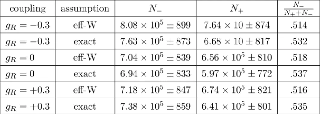
We shall start by considering the Standard Model tree-level predictions concerning single top production. In Table 2 and figure 3 we present our numerical results for production of polarized tops in the helicity basis and compare them to an the exact calculation of the cross-section. The error quoted is the √N statistical one. We have not included the errors associated to the approximations made in the effective W approximation. From this table we see that both polarizations appear roughly at a comparable rate, the number of negative helicity tops is just a mere 52% of the total. This is actually in very good agreement with the exact calculation presented in [16] provided that a) identicalpT and angular cuts are used in
coupling assumption N− N+ NN− ++N−
gR=−0.3 eff-W 8.08×10⁵±899 7.64×10±874 .514
gR=−0.3 exact 7.63×10⁵±873 6.68×10±817 .532
gR= 0 eff-W 7.04×10⁵±839 6.56×10⁵±810 .518
gR= 0 exact 6.94×10⁵±833 5.97×10⁵±772 .537
gR= +0.3 eff-W 7.18×10⁵±847 6.74×10⁵±821 .516
gR= +0.3 exact 7.38×10⁵±859 6.41×10⁵±801 .535
Table 2: Total number of events in single top production in the LAB helicity frame. The values were calculated varying the right effective coupling and keeping fixed the left one to the SM value. A comparison between results obtained with and without the effective W approximation is presented. Values calculated with pT > 30 GeV., 10◦ < θ < 170◦ and
√
s >500 GeV.
subprocess is used in both cases and c) no cuts are placed on the spectator quark in the exact calculation (recall that the spectator quark is invisible in the effective W approximation)
We have also calculated single anti-top production. In Fig.4 we show two different his-tograms corresponding to the production of ¯t with the two possible helicities in the LAB frame. All the histograms correspond to the tree level electroweak approximation and clearly show that single anti-top production is suppressed roughly by a factor of two with respect to single top production. This feature is general and is due to the different probability of extracting aW− from a proton as compared to that of extracting a W+. The relevant elec-troweak cross sections (see Appendix) are symmetric under the interchange of particle by antiparticle along with helicity flip.
In figures 5 and 6 we plot the angular distribution of single top production in the (tree-level) Standard Model and compare them to the exact calculation [16] with an equivalent set of cuts. From the inspection of these figures two facts emerge: a) as expected the distribution is strongly peaked in the beam direction, with the probability of top and anti-bottom being produced back to back or parallel being almost identical. The exact calculation has similar features, although favours slightly top and anti-bottom emerging in the same direction. b) The distribution is nevertheless flatter for right handed tops, showing more structure at large angles.
As we see, the predictions from the effectiveW approximation stand well in a comparison with the exact results up to this point. However, the degree of polarization is extremely small and it has little to do with the large polarizations reported in [11] or even with those found in [16] (which were slightly below the ones considered in [11].) In fact, everything can be understood in terms of the cuts and the different kinematical constraints that using the
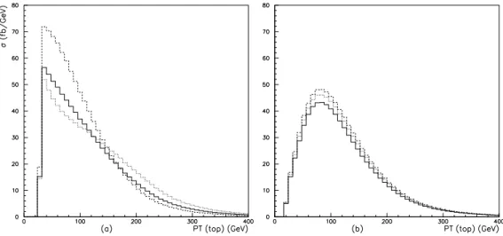
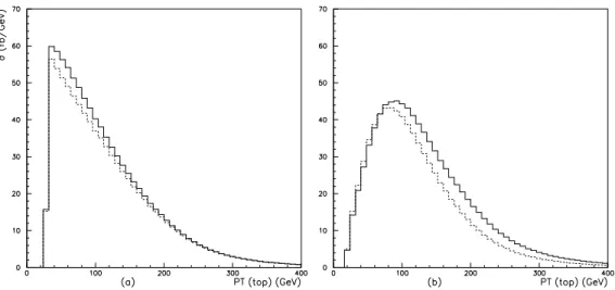
Figure 3: Differential cross section of (single) tops produced at the LHC vs. transversal mo-mentum in the Standard Model. The solid (dotted) line corresponds to left (right) polarized top production. The subprocesses contributing to these histograms have been calculated at tree level in the electroweak theory. In the figure we show the results of the calculations for polarized top production in the LAB helicity basis. These predictions (a) are compared to those of the exact calculation (b). We see that the agreement is reasonable forpT >100 GeV
[16], but fails at low values ofpT.
Figure 4: Differential cross section of (single) anti-top at the LHC vs. transversal momentum at tree level in the Standard Model. The solid (dotted) line corresponds to right (left) polarized anti-top production. All the histograms correspond to subprocesses calculated in the tree level electroweak approximation in the LAB helicity frame.
Figure 5: Expected angular distribution for single top production produced at the LHC in the Standard Model calculated in the effective W approximation.
Figure 6: Same as in the previous figure but with an exact calculation. The results of [16] have been used.
effective W approximation forces upon us.
Let us see this in some more detail. If in the exact calculation we set a cut on the pT
of the spectator quark identical to the one that was used in [16], the polarization jumps immediately from the 53 % to a (still modest) 58 % . If, on top of that, we place the angular cuts on the spectator quark that were used in [16] we get a 70% polarization in the LAB helicity frame. It is thus a judicious choice of the cuts what enlarges the polarization. In comparable situations the effective W treatment does actually quite well. It is thus quite suitable only for a treatment of the total cross section, and of course a lot easier and quicker to implement.
Let us now depart from the tree-level Standard Model and consider non-zero values for
δgLandδgR. Some numerical results are presented in table 2 for top production. The cuts are
as the ones employed so far. Further insight can be obtained by plotting thepT distribution.
Some of the results are presented in Fig.7. The results are somewhat disappointing in the sense that, particularly at low values of pT, the deviations with respect to the Standard
Model have a qualitative behaviour which is different from the one exhibited by an exact calculation. In the former the lineargLgR term clearly dominates, while in the latter the gR2
term has the upper hand. Still as we can see from Table 2 that the total cross section come out in reasonable agreement, the discrepancy lies basically in the profile of the distributions not in their total integrated value.
Like in an exact calculation, we have found that the positively polarized tops are more sensitive to the right handed coupling. This is not an unexpected result but not completely evident due to the large mass corrections for the top quark. However, it is clear that one has to work harder to extract, if at all, bounds on gR and one must necessarily use the exact
calculation.
6
Effective Couplings and Mixed States
In spite of the failure of the effectiveW approximation to yield the correct detailedpT
distri-bution when the right-handed coupling is turned on, it is clear that it provides a reasonably good description of the total cross section. Also, the discussion on the top polarization is particularly simple in these terms. For this reason we think that it is worthwhile to present here the following discussion concerning top polarization (see also [16]).
Using our results (including the effectiveW approximation) we obtain that the differential cross section matrix element at tree level can be written as (see Appendix for notation)
|M|2 =
|gR|2+|gL|2
a+
|gR|2− |gL|2
bn+mbmt
g∗RgL+gL∗gR
Figure 7: (a) Comparison between the tree Standard Model pT distribution for single
pos-itively polarized top production (solid line) and the corresponding obtained with a value
gR = ±0.3 for the effective right handed coupling (dotted/dashed line) in the effective W
approximation. (b) Same when the exact calculation is used. From the figures we can observe that the effective-W approximation distorts the gR dependence of the exact pT distribution
for all values of pT. Note however (see Table 2 for a numerical comparison) that the total
=
g∗R g∗L
a+bn mbmt
2 c
mbmt
2 c a−bn
!
gR
gL
!
(10)
≡ g∗R g∗L
A gR
gL
!
, (11)
wherea,bn, andcare independent of the effective couplingsgRandgLandbnis the only piece
that depends on the top spin four-vectorn.When|M|2 corresponds to the matrix element of the subprocess the exact expressions fora,bn, andccan be obtained from the formulae given
in the Appendix. For the matrix element of the whole process we have to multiply those expressions with the corresponding W and gluon parton distribution functions and make the summatories over parton species and polarizations but all this respects the general form given in Eq.(11). From Eq.(11) we can observe thatCP violating phases appear suppressed by the bottom mass but at the same time they are enhanced by a gL factor. Hence, if one
manages to find a highly polarized spin basis there are some chances of having experimentally observable effects. This is for sure not the case in the helicity basis as can be observed in table 2
For example for top and anti-top production in the LAB helicity frame, and after inte-grating over the kinematical variables, we haveN+ tops (anti-tops) with positive helicity and
N− tops (anti-tops) with negative helicity where
N+ =
|gR|2+|gL|2
atotal+
|gR|2− |gL|2
btotaln +mbmt
g∗RgL+gL∗gR
2 c
total
N =
|gR|2+|gL|2
atotal−
|gR|2− |gL|2
btotaln +mbmt
g∗RgL+gL∗gR
2 c
total
withatotal,btotaln and mbmtctotal for a right polarized top given by
atotal = 6.8×10⁵, btotaln = 0.24×10⁵, mbmtctotal = −1.5×10⁵,
where the usual set of cuts have been used. Returning to the discussion of the general aspects of Eq.(11) we observe thatA is a symmetric matrix and then it is diagonalizable. Moreover, from the positivity of|M|2 we immediately arrive at the constraints
detA = a2−b2n−m
2 bm2tc2
4 ≥0, (12)
1
2T rA = a≥0. (13)
In order to have a 100% polarized top we need a spin four-vector n that saturates constrain (12) for each kinematical situation, that is we needA to have a zero eigenvalue. In general
such n need not exist and, should it exist, is in any case independent of the anomalous couplings gR and gL. Moreover, provided this n exists there is only one solution (up to
a global complex normalization factor) for the pair (gR, gL) to the equation |M|2 = 0, or
equivalently to the eigenvector equation
A gR
gL
!
= 0, (14)
To illustrate these considerations let us give an example: In the unphysical situation where
mt → 0 it can be shown that there exists two solutions to the saturated constraint (12),
namely
mtnµ→ ±
|~p1|, p01 p~1
|p~1|
, (15)
once we have found this result we plug it in the expression (14) and we find the solutions (0, gL) with gL arbitrary for the + sign and (gR,0) with gR arbitrary for the - sign. That
is, physically we have zero probability of producing a right handed top when we have only a left handed coupling and viceversa when we have only a right handed coupling. Note that if our theory had a massless top and whatever non-null anomalous couplings gR and gL then
there would be no direction of 100% polarization. This can be understood remembering that the top particle forms in general an entangled state with the other particles of the process and since we are tracing over the unknown spin degrees of freedom of those particles we do not expect in general to end up with a top in a pure polarized state, although this is not impossible as it is shown the in above example. We postpone a detailed analysis of the top polarization within the effective -W approximation to a future publication
Although with such small degree of polarization (even in the minimal tree level Standard Model) the discussion becomes a bit academic, it is clear from the above analysis that if
gR6= 0 the top can never be in a pure state. We advise the interested reader to consult [16]
for more details.
7
Conclusions
We have done a complete calculation of the subprocess cross sections for polarized tops or anti-top production at the LHC including all mass corrections and with general effective couplings gLand gR. The calculations presented are fully analytical.
Then we have used those results to analyzed the single top production process at the LHC using the effective-W approximation. That is, considering that the W-boson is a real particle in order to calculate the probability of obtaining a W-boson from a proton as a product of probabilities. The effective-W approximation has in its favour its technical simplicity and a
clear physical interpretation for those used to the language of parton distribution function, being a generalization of the Weisz¨acker-Williams approximation for photons, which works exceedingly well.
In this work we have shown that the effective-W approximation is well suited to reproduce the rough features of the process. However from our results it clearly comes out that the distortion appearing in thepT distribution due to the presence of this approximation renders
it unsuited for any precise treatment of the single polarized top production problem. This can be clearly seen at lower values ofpT, in extensions of the minimal Standard Model when a
right handed coupling is included, where the effective-W approximation tends to enhance the linear terms ingR, which are screened by a largegR2 contribution in an exact calculation. At
the same time it is fair to say that if one considers the total cross section, the approximation fits much better the exact results and in particular the correct behavior under variations of the effective couplinggR is restored.
From those results our main conclusion is that as far as one is interested in total cross sections the effective-W approximation is a useful tool, but care must be taken when detailed
pT or angular distributions are needed.
8
Acknowledgments
It has been a pleasure to be able to present this work in the XXIX International Meeting on Fundamental Physics, in a special session devoted to the 60th birthday of Paco Yndur´ain, to whom this work is dedicated, with our best wishes of a long and productive career. We would like to thank A.Dobado, M.J.Herrero, J.R.Pel´aez and E.Ru´ız-Morales for multiple discussions. J.M. acknowledges a fellowship from Generalitat de Catalunya, grant 1998FI-00614. Financial support from grants AEN98-0431, 1998SGR 00026 and EURODAPHNE is greatly appreciated.
A
Subprocesses cross sections
In order to write the cross section of the subprocess, we define the spin four-vector corre-sponding to the spin in the ˆndirection as
nµ≡ q 1
p012−(~p1·nˆ)2
~
p1·n, pˆ 01nˆ,
with the properties
n2 = −1,
which reduces in the case of ±helicity (ˆn=±|~p~p1
1|) to nµ≡ ± 1
mt
|~p1|, p01 p~1
|p~1|
,
we have the differential cross section of the subprocess for single top production
dσ = fg(y)fu(x)fW(ˆx, E)dxdydxδˆ 4(k1+k2−p1−p2)
× 1
4k20~k1−k10~k2
Y2
f=1
d3pf
(2π)32Ef
|M|2(2π)4 and
|M|2 =g2sOijAij =gs2(O11A11+O22A22+Oc(A12+A21)),
where
O11 = 1
4 (k1·p1)2,
O22 = 1
4 (k1·p2)2,
Oc = O12=O21=
1
4 (k1·p1) (k1·p2),
and after averaging over gluon colours and transverse polarizations, and summing over fermion colours we have
A11 = A(+)11 +A11(−)+mtmbε2
gR∗gL+gL∗gR
2
m2t−k1·p1
+m2t
|gL|2+|gR|2 2 (ε·p2) (ε·(k1−p1))−ε2(p2·(k1−p1)) ,
with
A(11±) ≡ |g±|2ε·p2
2 ((k1−p1)·ε)
(k1−p1)·p1±mtn 2
−(k1−p1)2
ε·p1±mtn
2
− |g±|2 ε
2
2
2 ((k1−p1)·p2)
(k1−p1)·p1±mtn 2
−(k1−p1)2
p2·p1±mtn
2
+|g±|2 m
2 t
2
2 (ε·p2)
ε·p1∓mtn
2
−ε2
p2·p1∓mtn
2
,
and
A22=A(+)22 +A22(−)+mbmt
gR∗gL+g∗LgR
2 {p2·(p2−k1)}ε
2,
with
A(22±) ≡ |g±|2p2·(k2−p1)
2 (ε·(k2−p1))
ε·p1±mtn
2
−ε2
(k2−p1)·p1±mtn 2
−|g±|2
2 (k2−p1)
22 (ε·p 2)
ε·p1±mtn
2
−ε2
p2·p1±mtn
2
+m2b|g±|
2
2
2 (ε·(4k1−3p2))
ε·p1±mtn
2
−ε2
(4k1−3p2)·p1±mtn 2
and
A12+A21 = A(+)c +A(c−)
−mbmt
g∗RgL+gL∗gR
2
n
ε2[2 (p2·p1)−((p2+p1)·k1)] + 2 (ε·k1)2
o
+|gR|
2+|g L|2
2
2m2t(ε·p2) (ε·(k2−p1))−m2bm2tε2 ,
with
A(c±) = 2|g±|2(ε·p2)
(k1−p1)·p1±mtn 2
(ε·(k2−p1))
−
p1±mtn
2 ·(k2−p1)
(k1·ε)
−2|g±|2
ε·p1±mtn
2
{(ε·p2) (p1·(k1−p2)) + (ε·(k2−p1)) ((k1−p1)·p2)
−(ε·(k1−p1)) (p2·(k2−p1))} +|g±|2ε2
(p2·(k1−p1))
(k2−p1)·p1±mtn 2
+
p2·p1±mtn
2
((k2−p1)·(k1−p1))
−(p2·(k2−p1))
(k1−p1)·p1±mtn 2
−2|g±|2m2b(ε·(k1−p1))
ε·p1±mtn
2
,
whereεis the polarization of the W+ boson and
g+ ≡ gR,
g− ≡ gL,
For the subprocess of Fig.2 we have to perform the following changes in the expressions for the single top production.
ε ↔ ε∗, n ↔ −n, p2 ↔ −p2, p1 ↔ −p1, k2 ↔ −k2, k1 ↔ −k1,
but since we can take the W-boson polarization real and the cross section is even under the above sign changes, the subprocess cross section is the same for single top or anti-top production.
References
[1] A.N. Okpara,hep-ph/0105151 and proceedings for the 36th Rencontres de Moriond, QCD and High Energy Hadronic Interactions, Les Arcs, France, March 17 - 24, (2001)
[2] A.Dobado, D.Espriu and M.J.Herrero, Phys. Lett. B255 (1991) 405.
[3] M. E. Peskin, J. D. Wells, hep-ph/0101342;M.S. Chanowitz, Phys.Rev. D59 073005 (1999) and hep-ph/0104024
[4] T.Appelquist and C.Bernard, Phys. Rev. D22 (1980) 200; A.Longhitano, Phys. Rev. D22 (1980) 1166; A. Longhitano, Nucl. Phys. B188 (1981) 118; R.Renken and M.Peskin, Nucl. Phys. B211 (1983) 93; A.Dobado, D.Espriu and M.J.Herrero, Phys. Lett. B255 (1991) 405.
[5] T.Appelquist, M.Bowick, E.Cohler and A.Hauser, Phys. Rev. D31 (1985) 1676.
[6] See e.g. S.Catani, M.Mangano, P.Nason and L.Trentadue, Phys. Lett. B 378 (1996) 329
[7] D. Espriu, J. Manzano, Phys.Rev.D63 (2001) 073008
[8] T.M.P. Tait, Ph.D. Thesis, Michigan State University, 1999, hep-ph/9907462.
[9] S.Dawson, Nucl. Phys. B249 (1985) 42; S.Willenbrock and D.Dicus, Phys. Rev. D34 (1986) 155; C.P.Yuan, Phys. Rev. D41 (1990) 42; R.K.Ellis and S.Parke, Phys. Rev. D46 (1992) 3785; G.Bordes and B. van Eijk, Z. Phys. C 57 (1993) 81, Nucl. Phys. B435 (1995) 23; D.O.Carlson, Ph.D. Thesis, Michigan State University, 1995, hep-ph/9508278; T.Stelzer, Z.Sullivan and S.Willenbrock, Phys. Rev. D56 (1997) 5919.
[10] T.Stelzer, Z.Sullivan and S.Willenbrock,Phys. Rev. D58 (1998) 094021
[11] S.Parke, Proceedings of the International Symposium on Large QCD Corrections and New Physics, Hiroshima, 1997, Fermilab-Conf-97-431-T, hep-ph/9712512; G.Mahlon and S.Parke, Fermilab-Pub-99/361-T, hep-ph/9912458.
[12] M. Fischer, S. Groote, J.G. K¨orner and M.C. Mauser, hep-ph/0101322
[14] Z.-H. Lin, T. Han, T. Huang, J.-X. Wang , X. Zhang, hep-ph/0106344
[15] R. Peccei, X. Zhang, Nucl. Phys. B337 (1990) 269
[16] D. Espriu, J. Manzano, hep-ph/0107112
[17] T.Stelzer, Z.Sullivan and S.Willenbrock,Phys. Rev. D56 (1997) 5919
[18] M.C. Smith, S. Willenbrock, Phys. Rev. D54 (1996) 6696
[19] E.Bagan, D.Espriu, J.Manzano, Phys. Rev. D60, (1999) 114035.
[20] T. Affolder et al (CDF collaboration) hep-ex/0012029
[21] D.Amidei and C.Brock, Report of the the TeV2000 study group on future elec-troweak physics at the Tevatron, FERMILAB-PUB-96-082, 1996: S. Willenbrock, hep-ph/0103033
[22] T.Swarnicki (for the CLEO collaboration), Proceedings of the 1998 International Con-ference on HEP, vol. 2, 1057.
[23] F.Larios, M.A.Perez and C.P.Yuan, hep-ph/9903394; F.Larios, E.Malkawi, C.P.Yuan, Acta Phys. Polon. B27 (1996) 3741.
[24] C.Weisz¨acker and E.Williams, Z. Phys. 88 (1934) 244.
[25] S.Frixione, M.Mangano, P.Nason and G.Ridolfi, Phys. Lett. B319 (1993) 339.
[26] A. Dobado, M. J. Herrero, J. R. Pelaez, and E. Ruiz Morales, hep-ph/9912224
[27] CTEQ4: H.-L. Lai et al., Phys. Rev. D55 (1997) 1280, http://cteq.org.
[28] S. Dawson. Nucl.Phys. B249 (1985) 42-60.
[29] G.L.Kane, W.W.Repko and W.B.Rolnick, Phys. Lett., 148B (1984) 367.
[30] P.W.Johnson, F.J.Olness, and W.K.Tung, Phys. Rev. D36 (1987).
[31] B.Mele, in Proceedings of the Workshop on Physics at Future Accelerators, vol. II, p.13, J. Mulvey, ed. (1987).
[32] J.Lindfors, Z. Phys. C28 (1985) 427; R.Kauffman, Ph. D. Thesis, SLAC-0348 (1989).
![Figure 6: Same as in the previous figure but with an exact calculation. The results of [16]](https://thumb-us.123doks.com/thumbv2/123dok_us/8527689.2292389/16.918.322.590.632.884/figure-previous-figure-exact-calculation-results.webp)