Evolution strategies for robust optimization

Cover Page

The handle

http://hdl.handle.net/1887/18931

holds various files of this Leiden University

dissertation.

Author:

Kruisselbrink, Johannes Willem

Title:

Evolution strategies for robust optimization

Proefschrift

ter verkrijging van

de graad van Doctor aan de Universiteit Leiden, op gezag van Rector Magnificus prof. mr. P.F. van der Heijden,

volgens besluit van het College voor Promoties te verdedigen op donderdag 10 mei 2012

klokke 11:15 uur

door

Johannes Willem Kruisselbrink

Promotor: Prof. Dr. T.H.W. B¨ack

Copromotor: Dr. M.T.M. Emmerich

Overige leden: Prof. Dr. J. Branke (University of Warwick) Prof. Dr. B. Sendhoff (University of Darmstadt) Prof. Dr. J.N. Kok

Dr. W.A. Kosters

Het onderzoek beschreven in dit proefschrift is uitgevoerd aan het Leiden Institute of Advanced Computer Science (LIACS), Universiteit Leiden. De totstandkoming van dit proefschrift is financieel ondersteund door de Nederlandse Organisatie voor Wetenschappelijk Onderzoek (NWO), project 612.066.618 “RoDeO”.

1 Introduction 3

1.1 A Brief History . . . 4

1.2 Aim and Objectives . . . 6

1.3 Overview of this Thesis . . . 6

I

From Optimization to Robust Optimization

9

2.2 The Practical Goal of Optimization . . . 17

2.3 Objective Function Landscapes . . . 18

2.4 Single Objective Real-Parameter Landscapes . . . 19

2.5 Black-Box Optimization Algorithms . . . 20

2.6 Summary and Discussion . . . 22

3 Robust Optimization 23 3.1 Uncertainties and Noise in Optimization Problems . . . 23

3.2 Robust Optimization . . . 33

3.3 Real-World Robust Optimization Scenarios . . . 35

3.4 Summary and Discussion . . . 37

II

Evolution Strategies for Robust Optimization

39

4.2 Evolution Strategies . . . 43

4.3 Summary and Discussion . . . 54

5 Optimization of Noisy Objective Functions 55 5.1 Noisy Objective Functions . . . 56

5.4 Adaptive Averaging . . . 67

5.5 Metamodel Assisted Noise Handling . . . 92

5.6 A General Discussion of Noise Handling Techniques . . . 97

5.7 Summary and Discussion . . . 99

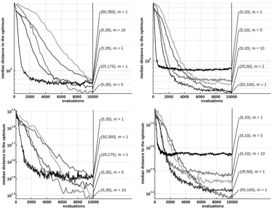
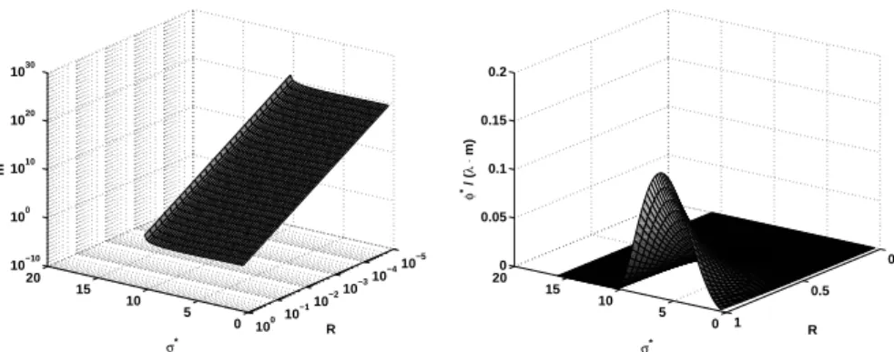
6 A Study on Noise Handling Schemes 101 6.1 The Growth Rate of the Sample Size . . . 101

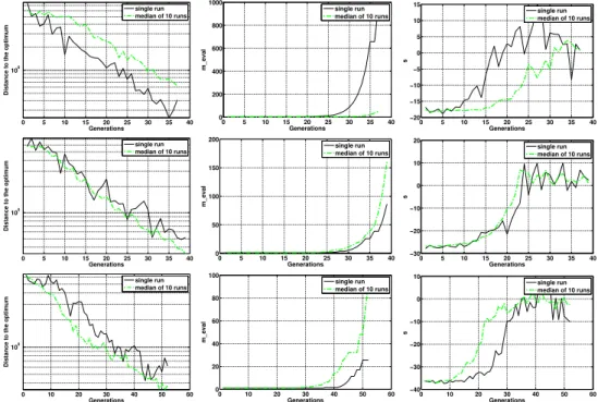
6.2 Tuning the Adaptive Averaging Methods . . . 107

6.3 Adaptive Versus Non-Adaptive Averaging . . . 115

6.4 Summary and Discussion . . . 132

7 Finding Robust Optima 133 7.1 Problem Definitions for Finding Robust Optima . . . 134

7.2 Strategies for Finding Robust Optima . . . 145

7.3 Summary and Discussion . . . 190

8 Empirical Study on Finding Robust Optima 193 8.1 Experimental Setup . . . 193

8.2 Tuning the Static Resampling Schemes . . . 195

8.3 Full Comparison of Schemes Finding Robust Optima . . . 206

8.4 Summary and Discussion . . . 212

9 Conclusion 213 9.1 Summary . . . 213

9.2 Outlook . . . 216

Bibliography 219

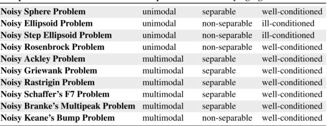
A Test Problems for Noisy Optimization 229

B Test Problems for Finding Robust Optima 241

C Kriging Metamodeling 251

Samenvatting (Dutch) 255

Introduction

When solving real-world optimization problems a frequently encountered difficulty is the presence of uncertainties and noise within the system for which optima are sought. Due to various reasons, various types of uncertainties and noise can arise in optimization problems. Hence, for real-world scenarios, optimization methods are needed that can deal with these uncertainties and solutions ought to be found that are not only optimal in the theoretical sense, but that are also practical in real life. The practice of optimization that accounts for uncertainties and noise is often referred to asrobust optimization.

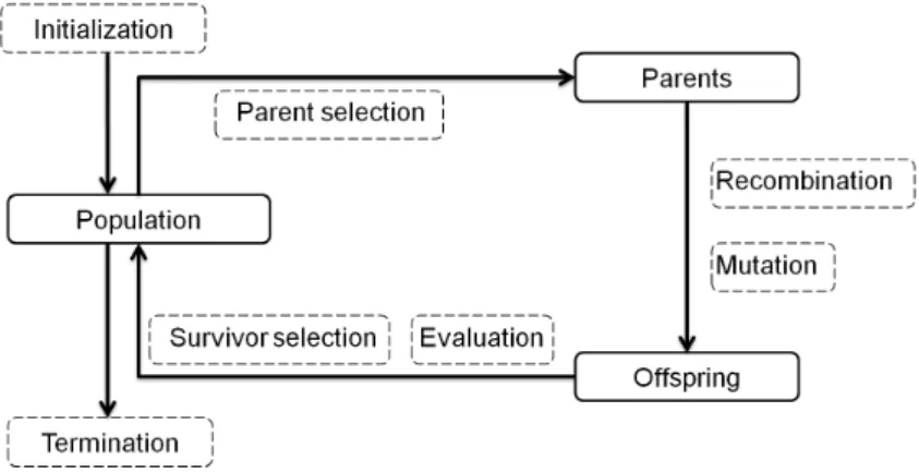
Evolutionary Algorithms (EAs) form a class of optimization algorithms that use the

principle of evolution to find good solutions to optimization problems. The paradigm of

evolutionary computationis simple and effective; take a population of candidate solutions for

the optimization problem and simulate the process of evolution to evolve the population toward better solutions. With applications in various real-world settings, Evolutionary Algorithms are well-established and have proven to be powerful for optimization, especially for complex problems that are difficult or impossible to solve analytically.

Evolutionary Algorithms are originally proposed for solving optimization problems that are not affected by uncertainties and noise. However, natural evolution seems to be inherently robust when viewing it as an optimization process, because uncertainty and noise are indis-pensable parts of nature. Being inspired by evolution in nature, one question is therefore to what extent the natural mechanisms adopted by Evolutionary Algorithms make them robust against uncertainties and noise. Additionally, when acknowledging the limited precision of natural evolution, the challenge is to make Evolutionary Algorithms even more effective in the scope of robust optimization.

In this work we will study the application of Evolutionary Algorithms, and in particular

Evolution Strategies, in the context of robust optimization. The main questions that we will

the optimization model? What can be done to fix or improve the behavior of Evolutionary Algorithms when dealing with uncertainties and noise?

1.1 A Brief History

The concept of robust (design) optimization originated from the concept ofrobust designin industrial engineering. The introduction, or better, popularization of this concept is generally attributed to Taguchi [Tag78, Tag86, Tag89]. Taguchi stated that for product design engineer-ing, a product should be designed not only for optimal performance, but also as to make the performance as insensitive as possible to variations that are beyond the designer’s control. He proposed a method based on simple experimental designs andloss functionsto incorporate the notion of quality or performance robustness into the process of design engineering. Taguchi bundled his ideas in a design method called theTaguchi method(see e.g., [Pha89]). Although the methodologies proposed by Taguchi have received much criticism [BST+88, AMB+92] and are considered to be outdated [CWZ99], the impact of the robust design philosophy cannot be neglected. The general aim of trying to take uncertainty and noise into account within the scope of product development has become a standard part of modern engineering [Par07]. In modern engineering, the increasing use of computer models to virtually test (parts of) designs has also led to increased interest in computational optimization techniques to aid the design process [EH02]. However, classical optimization methods focus mainly on finding op-timal solutions for exact, noise-free systems. Due to the frequently noisy and uncertain nature of real life, the increased application of optimization techniques for real-world applications led to the awareness that there are a number of problems that require ways of incorporating the notion of robustness in the measures of solution quality (which is the leading principle of robust design) in optimization techniques [Tro97, TAW03].

As noted by Trosset [Tro97], robust optimization is only a part of the broader concept of robust design. The general aim of obtaining high quality products often involves design of

experimentsmethods and sensitivity analysiswhere the optimization is performed manually

by means of statistical analysis. Only in some cases automated optimization is used to aid the design process, and robust optimization methods can be applied to find robust solutions.

[SJ08] is particularly worthwhile mentioning as it presents a large number of applications of robust optimization techniques within the field of mechanical engineering.

In Operations Research, the problem of dealing with uncertainties and noise comprises a number of variants. Studies that consider uncertainty in the optimization model date back to the work of Dantzig [Dan55] in 1955 and Wets [Wet66] in 1966. Today, approaches dealing with uncertainties can be found in various settings in the scope of mathematical programming; in the form ofstochastic programming (e.g., [KW94]), under the term robust optimization

[MVZ95, BTGGN04, BBC11], and in the scope offuzzy programming[BZ70, IR00] which knows the two types offlexible programming[TOA74, Zim76] andpossibilistic programming

[TA84]. In [Sah04], an overview can be found of the different mathematical programming classes that deal with uncertainty and noise, and the way in which these are modeled into optimization problems.

Also in the scope ofblack-box optimization, and particularly in the field of evolutionary computation, there is an increasing interest for methods that deal with uncertainty and noise. A summary of the way in which such optimization problems are approached within this field, and references to approaches proposed in literature can be found in [JB05].

Finally, some of the challenges and opportunities stated by Sahinidis [Sah04] in an overview of robust optimization using mathematical programming techniques also hold for the broader scope of optimization under uncertainty and noise. The following list of challenges, based on those stated by Sahinidis, forms the starting point of this thesis:

• An effort should be made to construct a unified framework which combines the different philosophies of modeling uncertainty and noise within optimization problems.

• Many approaches focus solely on one particular type of uncertainty and noise, whereas real-world optimization problems can exhibit multiple types. Hybrid approaches that can deal with various types of uncertainties and noise simultaneously can be the next step of robust optimization.

• Non-standard search spaces have received limited attention within the scope of optim-ization under uncertainty and noise. Extending the modeling framework and also the optimization approaches such that they also allow for optimization under uncertainty and noise in other domains (e.g., graph-like spaces) is a challenging next step.

1.2 Aim and Objectives

The first objective of the current work is to obtain a clear formulation of robust optimization. The term robustness is in itself a very general term, obtaining a clear view on the scope and goals of robust optimization is therefore essential. An objective emerging from this is to provide guidelines for systematic classification of various types of robust optimization problems.

The second objective is to bridge the gap from the formulation of robust optimization to the practice of robust optimization. The aim is to exemplify how to approach robust optimization problems. Moreover, we aim to study the behavior of Evolution Strategies on such problems and find how they should be adapted in order to better deal with such problems. For this, approaches from the literature and newly proposed ideas will be compared conceptually and empirically using two Evolution Strategy variants as algorithmic cores.

The third objective is to provide a framework for empirical comparison for the two robust optimization scenarios considered in this work. This is done by providing a small, focused set of benchmark problems and empirical results that can, in term, be used as benchmarks.

1.3 Overview of this Thesis

This work consists of two parts. In the first part, the aim is to form an exact conceptual picture of what robust optimization is, how it relates to traditional non-robust optimization, and what the implications are for solving real-world optimization problems. The second part of this work focuses on the application of Evolution Strategies (ES) targeted on solving real-parameter robust optimization problems. In particular two main scenarios of robust optimization are considered:optimization of noisy objective functions and finding robust optima. These are considered as frequently occurring and representative scenarios of robust optimization. For these two scenarios, the performance and possible ways of improvement of two particular Evolution Strategy instances, namely the(5/2DI,35)-σSA-ES and the CMA-ES, are studied.

Chapter 2 lays out the background by providing an overview on the classical view on

optimization, together with frequently used terms and concepts. This chapter forms the backbone of this work.

Chapter 3extends the classical view on optimization to a framework and definition of robust

optimization. It provides a taxonomy of the different ways in which uncertainties and noise can arise within optimization problems and a unified and concise framework for their systematic classification. This chapter is partially based on insights and results previously published in [KBIvdH08, KAE+09, KEB+09b].

Chapter 4introduces Evolutionary Algorithms and Evolution Strategies, therewith forming

Chapter 5discusses the application of Evolution Strategies to noisy objective functions. In this chapter, the negative effects of noise on Evolution Strategies are studied and techniques to counter the effects of noise in the objective function are compared conceptually. In Sec-tion 5.4.6 an alternative type of uncertainty quantificaSec-tion is proposed and discussed. This chapter uses results and insights that have been published partly in [KEB09a, KRD+11].

Chapter 6 focuses on a particular class of noise handling techniques, namely adaptive

averaging techniques. For these techniques the main question is how these compare to straight-forward ways of dealing with noisy objective functions. This chapter presents new results on accuracy limits for adaptive noise handling in Evolution Strategies with the theoretical results presented in Section 6.1 and the empirical comparisons of different noise handling schemes.

Chapter 7 focuses on the scenario of finding robust optima in anticipation of

uncertain-ties/noise in the design variables. The goal of finding robust optima is explicitly stated and formulated in the light of the framework of robust optimization. Different techniques that are proposed for finding robust optima are reviewed and compared conceptually. This chapter merges the individual results on algorithmic schemes of [KEDB10a, KEB10, KEDB10b, KRD+_{11] with each other and puts them into a global scope of existing studies.}

Chapter 8presents an empirical comparison of different strategies for finding robust optima.

This chapter presents new results with an empirical comparison of different techniques for finding robust optima, amongst which are the algorithms presented in [KEDB10a, KEB10, KEDB10b, KRD+_11].

Chapter 9closes with a summary and an outlook.

Optimization

This chapter lays out the background of this work by providing a summary of black-box optimization. It introduces the “classical” view on optimization together with the concepts and terminology that are commonly used within this context. This classical view on optimization will be extended in Chapter 3 to form a definition of robust optimization.

Section 2.1 starts with providing a global description and a formal definition of a black-box optimization problem as it will be used in this thesis. Section 2.2 discusses how the practice of optimization is generally perceived in practical applications. Section 2.3 zooms in on the concept of objective function landscape, which is a frequently used metaphor for perceiving optimization problems. Section 2.4 focuses on real-parameter optimization problems, being the main type of optimization problem discussed in this thesis. Section 2.5 provides an overview of black-box optimization algorithms and the general goal of automated optimization. Section 2.6 closes with a summary and discussion.

2.1 Optimization Problems

The model of Figure 2.1 describes an optimization problem. It considers a system that produces outputyas a function of inputx. Keeping it as general as possible, we note thatxandy can be of any form and assume that there is no knowledge about the internal mechanisms of the system, i.e., it is considered to be a black-box. Given such a system and a large number of possible input settings, the central problem of optimization can be loosely formulated as:

What setting(s) of the inputxyield(s) the best possible (optimal) outputy?

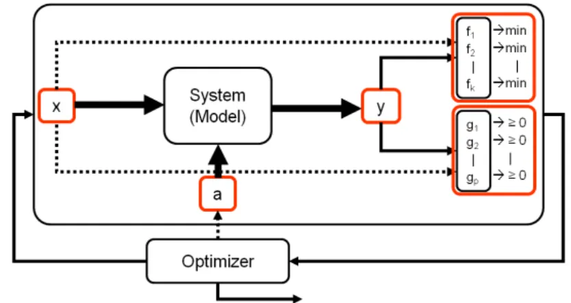
Figure 2.2: The general model of an optimization problem.

To deal with problems of this type, the model of Figure 2.1 is commonly transformed into a form as depicted in Figure 2.2. In many cases the system that is considered is replaced by an abstract model of the system (e.g., a mathematical model or a simulator). Furthermore, one or more objective functionsf1, . . . , fk and optionally also a number of constraint functions

g1, . . . , gp are introduced. The objective functions are of the form fi : X × Y → Rand

assign score values to each inputx ∈ X based on its respective outputy ∈ Y. Note that we could also neglect the intermediate mapping X → Y, which yields the more common formfi : X → R. Without loss of generality, we assume that each score function is to be

minimized. The constraint functions are of the formgi:X × Y →Rand rate the feasibility of

each possible inputx, again usingy. Also here the intermediate mapping could be neglected to obtain the more common formgi : X → R. For a possible inputx, it should hold that

gi(x)≥0in order forxto be feasible1.

The model of an optimization problem of Figure 2.2 can also be described mathematically:

Definition 2.1.1 (Optimization Problem):An optimization problem is a triple (X,F,G),

where:

• Xis the search space, which is the nonempty set of all possible solutions.

• F = {f1, . . . , fk},k ∈ N1, is a set of one or more objective functions that are to be

minimized. Each objective function is a function of the formf : X → Rthat maps

elements of the search space to a score value.

• G={g1, . . . , gp},p∈N0, is a set of constraint functions that need to be satisfied. Each

constraint function is of the formg :X →Rmapping elements of the search space to

a constraint value. For a certain inputx∈ X a constraintgis said to be satisfied if and only ifg(x)≥0. Otherwise, ifg(x)<0, then solutionxviolates the constraint and is therefore infeasible.

1_{Constraints of the formg(x) ≥ 0are referred to as inequality constraints. In literature, also another type of} constraint is used, namely the equality constraint, which is of the formh(x) = 0. In the definition given here, equality constraints are not included because they can easily be constructed using two inequality constraints (i.e.,

Furthermore, we use the following definition of feasibility:

Definition 2.1.2(Feasible Solution and Set of Feasible Solutions):For an optimization

prob-lem(X,F,G), theset of feasible solutionsAis the set

A={x∈ X |gi(x)≥0, i= 1, . . . , p}, (2.1)

and each solutionx∈ Ais called afeasible solution.

Given a problem that fits Definition 2.1.1, the goal of optimization can still vary and roughly be of one of the following forms:

1. Findafeasible solution that is optimal with respect to the objective function(s). 2. Findallfeasible solutions that are optimal with respect to the objective function(s). 3. Finda specific set of feasible solutions that are optimal with respect to the objective

function(s).

Here, “a specific set of solutions” loosely denotes the cases where, either implicitly or explicitly, also a secondary set selection criterion encompasses the optimization problem (e.g., searching for a diverse set of solutions requires a diversity notion based on sets of solutions). In addition to these three aims, a second class of optimization goals can also be identified in which the aim is to find solutions of which the objective function value(s) satisfies/satisfy (a) certain threshold value(s):

4. Find a feasible solution of which the objective function value(s) satisfies/satisfy (a) certain threshold value(s).

5. Findallfeasible solutions of which the objective function value(s) satisfy (a) certain threshold value(s).

6. Finda specific set of feasible solutions of which the objective function value(s) satisfy (a) certain threshold value(s).

Note that the latter three aims could also be seen as constraint satisfaction problems (i.e., an objective function with a threshold is effectively a constraint function).

Given the definition of an optimization problem and the loosely defined possible goals of optimization, next we will give more formal definitions of optimality. However, in order to do this, we will make a distinction betweensingle objective optimization problemsand

multi-objective optimization problemsand provide separate definitions for both classes.

2.1.1 Single Objective Optimization Problems

Definition 2.1.3 (Single Objective Optimization Problem):A single objective optimization

problem is an optimization problem with precisely one objective function. For the triple

(X,F,G), the setFconsists of exactly one objective function (k= 1in Definition 2.1.1). Given a single objective optimization problem, based on the definition of T¨orn and ˘Zilinskas [TZ89], B¨ack [B¨ac96] defines theglobal optimization problemas the problem of determining a global minimizer:

Definition 2.1.4(Global Minimum/Optimum and Global Minimizer/Optimizer):For a single

objective optimization problem(X,F,G)withF={f}and a set of feasible solutionsA, the

global minimumorglobal optimumf∗is the value

f∗= min{f(x)|x∈ A}, (2.2)

and every solutionx∗ ∈ Afor which it holds thatf(x∗) =f∗is called aglobal minimizeror

global optimizer.

This definition falls into the first item of the enumeration on page 13. Moreover, there are two other important remarks that have to be made. First, it is important to realize that there exist objective functions for which no global minimum exists. This can happen for objective functions of which the imagef[A]off :A →Ris non-compact (e.g., the infimum off[A]is

not included inf[A]). Secondly, one should note that when a global optimum does exist, there is only one global optimum, but there might be multiple global optimizers.

As it might happen that there are multiple solutionsxfor which holds thatf(x) = f∗, an extended goal of global optimization is to find all global minimizers (see [TZ89]):

X∗={x∈ A |f(x) =f∗}. (2.3)

This extended goal falls into the second item of the enumeration above.

The alternative goals of finding solutions with objective function values satisfying a certain threshold value (items 4–6 in the enumeration on page 13) are for single objective optimization problems known assuper/sub level setoptimization problems:

Definition 2.1.5(Sublevel Set):For a single objective optimization problem(X,F,G)with

F={f}and set of feasible solutionsA, thesublevel setbelow leveldis the set

Ld={x∈ A |f(x)≤d}. (2.4)

2.1.2 Multi-Objective Optimization Problems

A multi-objective optimization problem is a special instance of an optimization problem, defined as

Definition 2.1.6 (Multi-Objective Optimization Problem):A multi-objective optimization

(X,F,G), the setFconsists of at least two objective functions.

For multi-objective optimization problems, the definition of optimality is often based on the notion of Pareto dominance on the objective space. Pareto dominance introduces a partial order on the space of objective function values, beingRk for a problem withk objectives. In the

context of minimization, this order is defined as:

Definition 2.1.7(Pareto Dominance, Weak Pareto Dominance, Strict Pareto Dominance, and

Incomparability):For any two vectorsuandv:

udominatesv(notationu≺Paretovor justu≺v) iff:

∀i∈ {1, . . . , k}:ui ≤vi (2.5)

and ∃j∈ {1, . . . , k}:uj< vj, (2.6)

uweakly dominatesv(notationuv) iff:

uv∨u=v, (2.7)

ustrictly dominatesviff:

∀i∈ {1, . . . , k}:ui< vi, (2.8)

uandvareincomparable(notationu||v) iff:

uv∧vu. (2.9)

The partial order introduced by using the notion of Pareto dominance on the solution space can be used to define the goal of multi-objective optimization as to find Pareto optimizers:

Definition 2.1.8(Pareto Optimizer and Pareto Optimum):For a multi-objective optimization

problem(X,F,G)with a set of feasible solutionsA, theset of Pareto optimal solutionsX∗

is the set of all solutionsx∗ ∈ A with function values f(x∗) = [f1(x∗), . . . , fk(x∗)] for which it holds that there does not exist another solutionx∈ Awith function valuesf(x) = [f1(x), . . . , fk(x)]such thatf(x)dominatesf(x∗). I.e.,

X∗={x∗∈ A |@x∈ A:f(x)≺f(x∗)}. (2.10)

An element of the set of Pareto optimal solutionsx∗∈X∗is called aPareto optimizerand its objective function value vector is called aPareto optimum.

Although for some multi-objective optimization problems it is sufficient to find a Pareto optimal solution, in general, when a problem is defined as a multi-objective optimization problem, it is intended also to get insight in the trade-offs between the various objectives. Therefore the more usual (customary) aim for multi-objective optimization is to find the set of all Pareto optimal solutions or at least a representative subset of it.

(X,F,G), the set of all Pareto optima is called the Pareto Front and the set of all Pareto optimizers is called theEfficient Set.

With the definitions for a single- and multi-objective optimization problem, and the goal to find either one, multiple, or all optimizers, the basic problems of optimization have been introduced. How to solve optimization problems is another matter.

2.1.3 Discrete versus Real-Parameter Optimization Problems

Definition 2.1.1 only generally specifies the search spaceX, the objective functionsF, and the constraint functionsG. Besides the separation of single- and multi-objective optimization problems, another distinction can be made by looking at the search space. Although it is not a comprehensive categorization, we distinguish two major classes of optimization problems:

discrete optimization problemsandreal-parameter optimization problems.

Discrete optimization problems (which is a class that includescombinatorial optimization

problems) are optimization problems where the search space is a discrete set of candidate

solutions.

Definition 2.1.10(Discrete Optimization Problem):Any optimization problem of which the

search space is a discrete set is called adiscrete optimization problem.

This work focuses on the class of real-parameter optimization problems. Real-parameter optimization problems are optimization problems where the search space is a real-valued parameter space.

Definition 2.1.11 (Real-Parameter Optimization Problem):A real-parameter optimization

problemis an optimization problem(X,F,G), withX ⊆_Rn _{andX is of dimension nfor}

some fixedn∈N1.

More specifically, for real-parameter optimization problems commonly a stricter class defin-ition is taken, requiring the search space to be bounded by a box. We identify such types of problems as box-constrained real-parameter optimization problems.

Definition 2.1.12 (Box-Constrained Real-Parameter Optimization Problem):A

box-constrained real-parameter optimization problemis a real-parameter optimization problem

(X,F,G), with

X ={x∈_Rn_|(x

l)i≤(x)i≤(xu)i, i= 1, . . . , n}, (2.11) for some fixedn ∈ N1, and wherexl ∈ Rn is a vector of lower bounds andxu ∈ Rn is a

vector of upper bounds.

2.2 The Practical Goal of Optimization

Given the definition of an optimization problem, the rough classification of optimization goals, the distinction between single- and multi-objective optimization, and the rough classification of discrete versus real-parameter optimization problems, the question is: How to solve such problems? The solvability of optimization problems much depends on the structure of the search space and the basic assumptions about the objective and constraint functions.

Discrete optimization problems with finite (enumerable) search spaces are solvable within a finite number of steps by means ofcomplete enumeration. That is, by evaluating every solution in the search space it is possible to determine all optimizers. However, this has practical limits, for example when the search space is sufficiently large and/or evaluations are very time/cost expensive. Given that it is not possible to evaluate all candidate solutions we can follow the reasoning of B¨ack [B¨ac96] that when a strict subset of the search space is evaluated it is possible that the global optimum of a functionf differs arbitrarily much from the optimum found so far. Hence, if we cannot afford to evaluate every solution in the search space, an optimization problem is generally unsolvable.

For real-parameter optimization problems an even more discouraging observation was made by T¨orn and ˘Zilinskas [TZ89] who in the context of single objective optimization, according to B¨ack [B¨ac96], proved that

“The problem of determining a member of the level set Lf∗₊ of an arbitrary

global optimization problem on a real-parameter objective functionf on a

com-pact feasible region M within a finite number of steps is unsolvable.” [B¨ac96,

p. 37]

Note that a similar message can be deduced for multi-objective optimization.

Given this observation, we can state that global optimization problems as generally formulated by Definition 2.1.1 on page 12 are practically unsolvable unless we a) restrict ourselves to a class of optimization problems for which the objective functions satisfy certain additional conditions, or b) relax the solvability requirement [TZ89]. Both are done in practice. Regarding the class of problems that is considered, it is commonly assumed that the optimization problem exhibits some kind of underlying structure. An implicit assumption that is often made is that similar solutions are believed to have similar performance. While agreeing that the notion of similarity is not well-defined, neither its intuitiveness nor its validity can be denied. The goal of optimization is relaxed by taking a more practical viewpoint. Based on the definition provided by T¨orn and ˘Zilinskas [TZ89] we define the general goal of optimization as:

Definition 2.2.1 (Practical Goal of Optimization):Given an optimization problem with an

budget), thepractical goal of optimizationis to use these resources in an optimal way to find (an) as good as possible solution(s).

Or, from a slightly different perspective, one could aim for finding solutions that are an improvement with respect to the currently best known solution (melioration).

In addition to the practical goal of optimization, it is generally noted that an optimization algorithm is aglobal optimization algorithmif, given an infinite evaluation budget, it will get arbitrarily close to the global optimum.

Definition 2.2.2(Global Optimization Condition):Letxtdenote the best solution found by the

optimization algorithm at timetwith function valueft. We say that the optimization algorithm satisfies theglobal optimization conditioniff fort → ∞,ft−f∗ < , for arbitrarily small positive values of.

Note that this goal is constructed in terms of finding one global optimizer (provided that it exists) and it should be extended when the goal is to find all (or a particular set of) global optimizers or level set solutions.

2.3 Objective Function Landscapes

A central dogma of geography formulated by Tobler is: “everything is related to everything else, but near things are more related than distant things” [Tob70]. This dogma represents an implicit assumption that is generally also used for optimization problems in practice, namely that there is a correlation between the (dis)similarity of two candidate solutions and the (dis)similarity of their objective function values. The conceptual step from a (dis)similarity measure to a distance measured : X × X → Ris commonly a small one, leading to the

assumption of the search space being a metric space(X, d)(e.g., Euclidean distance for real-parameter search spaces).

solution, repeating until no further improvements can be found. Hence, when viewing it from a maximization perspective, it takes steps uphill into the direction of the global optimum. A well-known example of a hill-climbing algorithm (for minimization) is theSteepest Descent

algorithm (see, e.g., [NW06]) that follows the path of the gradient.

For optimization algorithms that use operators based on local perturbations (such as hill-climbing algorithms, but also Evolutionary Algorithms), the objective function landscape metaphor can be used to visualize different geographical scenarios that have a different impact on the performance of these algorithms. For instance, when an objective function landscape consists of multiple peaks of different heights, a hill-climber can get stuck in one of the lower height peaks, i.e., a locally optimal solution. Interestingly, one can herewith observe that a hill-climbing algorithm does not satisfy the global optimization condition of Definition 2.2.2 and is therefore qualified as alocal optimization algorithm. This supports the viewpoint of objective function landscapes as a practical way to analyze optimization algorithms.

2.4 Single Objective Real-Parameter Landscapes

For single objective real-parameter optimization problems, the different geological concepts that can influence the behavior of perturbation-based optimization algorithms can formally be defined. Below, the most important concepts will be formalized exactly based on Euclidean distance as dissimilarity measure:

Definition 2.4.1(Weak Local Minimizer/Optimizer):For a single objective optimization

prob-lem(X,F,G)withF ={f}and the set of feasible solutionsA, aweak local minimizeror

weak local optimizeris a solutionx∗∈ Afor which it holds that

∃δ∈_R>0(∀x∈ A(||x−x∗||< δ⇒f(x∗)≤f(x))). (2.12)

Definition 2.4.2(Strict Local Minimizer/Optimizer):For a single objective optimization

prob-lem(X,F,G)withF ={f}and the set of feasible solutionsA, astrict local minimizeror

strict local optimizeris a solutionx∗∈ Afor which it holds that

∃δ∈R>0(∀x∈ A(||x−x∗||< δ∧x6=x∗⇒f(x∗)< f(x))). (2.13)

Definition 2.4.3(Weak/Strict Local Minimum/Optimum):For a single objective optimization

problem(X,F,G)withF = {f} and the set of feasible solutionsA, a(weak/strict) local

minimumor(weak/strict) local optimumf∗is a value for which there exists a weak/strict local

minimizer/optimizerx∗such thatf∗=f(x∗).

Definition 2.4.4(Unimodal, Multimodal and Multiglobal):An objective function is said to be

unimodalif it has only one optimizer (i.e., only a global optimizer). Otherwise, it is said to be

multimodal. A landscape is calledmultiglobalif there are several global optimizers.

Besides the existence of local optima and global optima, another phenomenon in objective function landscapes is the possible existence of plateaus. A plateau is defined as:

Definition 2.4.5(Flat Region and Plateau):For a single objective, real-parameter optimization

problem(X,F,G)withF={f}and the set of feasible solutionsA, aflat regionoff|Ais a

connected set of pointsP⊆ Asuch that

∀x∈P(f(x) =c) and∀x∈P(∃x>0 (Bx(x)∩ A ⊆P)), (2.14)

for somec∈R, withB(x) ={x0 ∈Rn| ||x−x0||< }, and withxdefined separately for

eachx∈ P. AplateauP is a flat region with the additional property that there exists no flat

regionP0⊃P.

Note that when considering the possible existence of plateaus, there are solutions within a plateau that are both weak local minimizers and weak local maximizers, namely the solutions x∗∈ Afor which it holds that

∃δ∈R>0(∀x∈ A(||x−x∗||< δ⇒f(x∗) =f(x))). (2.15)

This is a somewhat paradoxical property that emerges from using Definition 2.4.1. However, the alternative of restricting to Definition 2.4.2 and changing the≤-sign by the<-sign leads to the problem that in a similar case, the global optimum is not a local optimum.

2.5 Black-Box Optimization Algorithms

An optimization algorithm is an algorithmic method that can be applied to solve (a specific class of) optimization problems. There is a wealth of optimization methods available and choosing one for solving a given optimization problem depends much on the characteristics of the optimization problem at hand. There are many aspects that vary from problem to problem. Many optimization methods are especially designed for specific types of search spaces, objective and constraint functions, or tailored for special objective function classes.

Figure 2.3:The general setup for black-box optimization.

Figure 2.3 visualizes the general black-box optimization loop. The principle is straight-forward: An optimizer is coupled to the (model of the) system of interest (according to the model of Section 2.1). The optimizer generates one or more candidate solutions, feeds it/them to the system, and receives a quality score of these candidate solutions. Using this information, the optimizer generates a new set of candidate solutions, and again feeds those to the system to obtain their quality. This loop is repeated until either a satisfactory solution is found, a predefined evaluation budget has been reached, or any other termination criterion has been reached. Note that the term optimizer is used in two ways: for optimal solutions and for optimization algorithms. Evolutionary Algorithms form a sub-class of black-box optimization algorithms.

2.5.1 Quality Measures for Optimization Algorithms

A difficult issue in the field of black-box optimization is the assessment of the quality of optimization algorithms. The quality of an optimization algorithm depends much on the characteristics of the problem at hand and the class of optimization problems for which the algorithm is designed. Benchmark sets of test problems are often used for empirical comparison of multiple optimization algorithms, see, e.g., [SHL+_{05, HFRA09b, HFRA09a,}

HFRA10]. For these benchmark sets, there are two types of indicators that can be used for determine the quality of the optimization algorithm: The quality of the (set of) solution(s)

1. versus the number of objective function evaluations needed to obtain that quality, or 2. versus the total computation time needed to obtain that quality.

2.6 Summary and Discussion

In this chapter the background of this work is summarized, being the traditional view on black-box optimization. Given this view on optimization, the two main distinctions between single- and multi-objective optimization problems and between discrete- and real-parameter optimization problems are presented. For such problems, it is shown that there is a distinction between the theoretical goal of optimization and how this goal is used in practice.

Furthermore, the concept of objective function landscapes is summarized, which is based on the assumption that the search space is a metric space and that there is a correlation between (dis)similarity of two solutions and their objective function values. In particular, definitions of commonly used terms are given in the context of single objective real-parameter optimization problems. These types of problems are the main focus of this work.

Black-box optimization algorithms are algorithmic methods that aim to solve optimization problems. Such algorithms sequentially test candidate solutions in a trial-and-error fashion in order to find optimal solutions. Spatial correlation is commonly exploited by optimization algorithms, such as hill-climbing algorithms. Although the quality of an optimization algorithm much depends on the problem at hand, benchmark sets of test problems can be used for empirical comparison of optimization algorithms for certain problem classes.

Robust Optimization

The traditional view on optimization as presented in Chapter 2 does not account for uncer-tainties and noise. However, this is not realistic for many real-world optimization problems. Consider, for instance, industrial engineering applications. A common optimization scenario is that a non-deterministic simulator replaces the real-world system and the aim is to find solutions such that the real-world realizations of these solutions are of a good quality, also when these are slightly perturbed due to manufacturing errors. In this scenario, uncertainties and noise arise in various ways, e.g., in the form of uncertainty because an approximate model is used instead of the real-world system, in the form of noise because the simulator is non-deterministic, and in the form of uncertainty introduced by the inability to generate exact realizations of the solutions. These observations give rise to two new questions: In what way can uncertainties and noise arise in the general model of an optimization problem as presented in Section 2.1? How do we account for this when optimizing on such systems?

The structure of this chapter is as follows: Section 3.1 starts with an overview/taxonomy of the various ways in which uncertainties and noise can emerge in optimization problems. In Section 3.2, the scope and goals of robust optimization are derived from this taxonomy. Section 3.3 presents three real-world optimization scenarios and discusses them in the context of robust optimization. Section 3.4 closes with a summary and discussion.

3.1 Uncertainties and Noise in Optimization Problems

Often, due to a variety of reasons, the theoretical model used for optimization differs from the real-world system for which optimal solutions are desired. Examples are:

1. The design variables cannot be controlled with unlimited precision. (input)

2. The operational (or environmental) conditions fluctuate or are known only to a certain extent. (model)

4. Approximation models replace the real-world system within the optimization loop.

(model/output)

5. There is a degree of vagueness in the objectives and/or the constraint boundaries.

(objectives/constraints)

These uncertainties can have a negative impact on the practical applicability of using idealized models or assumptions for solving real-world optimization problems. Not accounting for uncertainty and noise might lead to solutions that are found to be optimal with respect to the idealized model, but which are not useful or performing optimally in practice.

For optimization problems, the terms uncertainty and noise refer to behavior in any part of the optimization model that can not (fully) be predicted or controlled, or that is subject to vagueness. As illustrated, the causes of uncertainties and noise in real-world optimization problems can be manifold. In order to find good methods to deal with uncertainties and noise, a first step is to distinguish the different classes of uncertainty and noise that can arise in optimization problems. Among the different ways in which such a classification can be made (see, e.g., [BS07, JB05, ONL06]), the classification provided in this section will, to a great extent, follow the categorization of Beyer and Sendhoff [BS07].

3.1.1 Sources of Uncertainty and Noise

One way to distinguish different types of uncertainty and noise within optimization problems is to categorize them by looking at the parts of the optimization model in which they arise. When considering the model illustrated in Figure 2.2, one can identify five different locations where uncertainty and/or noise can enter the optimization model (see Figure 3.1):

A) Uncertainties and/or noise in the design variables

B) Uncertainties and/or noise in the environmental parameters C) Uncertainties and/or noise in the output

D) Vagueness in the constraints

E) Preference uncertainty in the objectives

These sources of uncertainty/noise are integrated in different ways in the mathematical formu-lations of an optimization problem.

A) Uncertainties and/or noise in the design variables

Figure 3.1: The general optimization model showing the different parts of the systems in which uncertainties can arise.

which is the main type of uncertainty considered by the robust design concept. This type of noise gives rise to two different scenarios:

Scenario 1: A simulation model replaces the real-world system within the optimization

model. In this case the simulator accepts inputs as non-disturbed inputs, though in practice, solutions cannot be realized with unlimited precision. This can be compensated for by focusing the optimization on finding solutions that are also of high quality when slightly perturbed (i.e., finding robust optima).

Scenario 2: The real-world system is enclosed in the optimization loop (experimental

optimization). In this case the disturbances in the input propagate through the output,

hence to the objective and constraint functions. When the disturbances in the design variables can be measured a posteriori, the optimizer will receive deterministic meas-urements, but the sampling process cannot be controlled. In case that the disturbances cannot be measured a posteriori, these disturbances simply yield noise in the objective and constraint functions. The noise distributions can be of any kind depending on the distribution of the noise in the design variables, transformed through the output and the objective and constraint functions.

The effect of variations caused by uncertainties or noise in the design variables can be modeled within the formulation of an objective functions as:

˜

fi(x) =fi(x+δx), i= 1, . . . , k. (3.1) And similarly for the constraint functions:

˜

observation is that this noise or uncertainty can depend on the values of the design variables themselves, i.e., it can vary for differentx. Furthermore, due to this remodeling, the outputs of the objective and constraint functions become random variables (in case the uncertaintyδxcan be modeled as a random variable) or sets of possible outputs.

B) Uncertainties and/or noise in the environmental parameters

Uncontrollable (environmental) parameters of a system are not considered in the clas-sical optimization model as presented in Section 2.1 (see Figure 2.2). These parameters are in the classical view considered to be constants of the system. However, in practice many of such constants are noisy or uncertain. Fluctuating or unknown operating condi-tions and deficiencies of internal parameters are possible ways in which uncertainties can manifest themselves within this part of the optimization model. Similar to uncertainties in the design variables, the setting in which this type of uncertainty can be actively compensated for is when a simulation model replaces the real-world system within the optimization model. Otherwise, the uncertainty propagates to the objective and constraint functions.

To incorporate such scenarios into the model presented in Section 2.1, we extend it as follows: Let the set C denote the (possible) settings of uncontrollable environmental parameters of the system. The models of the objective and constraint functions are extended by also being a function of the environmental parameters, i.e.,f :X × C →R

for allf ∈ Fandg:X × C →_Rfor allg∈ G.

The effect of variations caused by uncertainties or noise in the environmental parameters can be modeled in the objective functions as:

˜

fi(x, a) =fi(x, α), i= 1, . . . , k. (3.3) And similarly for the constraint functions:

˜

gj(x, a) =gj(x, α), j= 1, . . . , p. (3.4) Hereα∈ Cis a noisy or uncertain counterpart of the constanta∈ C. As can be seen, by modeling the uncertainty/noise in this way, the constant environmental parametersaare replaced by random or uncertain variablesα.

C) Uncertainties and/or noise in the output

Note that both types could be present simultaneously, e.g., when using non-deterministic simulation models.

Noise or uncertainty in the output can be modeled within formulations of the objective functions as:

˜

fi(x) =fi(x) +zfi(x), i= 1, . . . , k, (3.5)

and in the constraint function definitions as:

˜

gj(x) =gj(x) +zgj(x), j= 1, . . . , p, (3.6)

withzfi(x)andzgj(x)being random/uncertain variables (possibly indexed by space),

denoting the propagation of the output uncertainty/noise to the objective and constraint functions.

Note that, strictly seen, the noise in the objective and constraint functions is a product of the noise in the output. Internally,zfi(x)is a (possibly non-linear) function of the noise

in the output, i.e., y(x) +zy(x). However, as we have chosen to model the objective functions and constraint functions in terms ofx, this cannot be modeled explicitly. Furthermore, note that uncertainties in the design variables and environmental paramet-ers in principle propagate as a noisy or uncertain output, i.e., fluctuating/uncertain design variables and environmental parameters yield fluctuating/uncertain system output.

D) Vagueness in the constraints

Often it is hard to obtain strict and bounded definitions of constraints. When dealing with constraints like “the temperature should not be too high” or “the risk should not be too high”, it is not possible (or desirable) to draw a straight line between satisfied and not-satisfied. Such vagueness calls for methods that can account for this (e.g., by using fuzzy logic techniques [Zad65, BZ70]).

Fuzzy constraints can be described using the following notation:

gj(x)&0. (3.7)

Here, _& is the fuzzified version of ≥ having the linguistic interpretation “gj(x) is essentially greater than0”. However, this notation does not take into account the degree to which the constraint is fuzzy. For example, considering the “temperature should not be too high” example, the notation of Eq. 3.7 does not specify the margins for which the temperature could still be acceptable.

Figure 3.2: A simple linear membership function.

grey area (or transition area), and the higher the value of the membership function, the higher the degree of satisfaction. Figure 3.2 illustrates the basic idea of a membership function. Mathematically, this transformation has the following form:

g(x)≥0 becomes Vg(g(x))→max. (3.8) A design issue that is introduced is that appropriate membership functions have to be constructed.

E) Preference uncertainty in the objectives

Preference uncertainty emerges when having multiple conflicting objectives, hence, when highly subjective trade-off choices have to be made regarding the importance of objectives. Preference might only be known afterwards, depending on the quality level that can be achieved for the objectives and the particularities of the trade-offs that exist. Approaches that use aggregate objective functions which combine multiple objectives functions into one objective function are prone to such uncertainties. Approaches that aim to approximate the complete Pareto frontier postpone such preference decisions. Of these five sources of uncertainty, a distinction can be made between the first three (A, B, and C) and the last two (D and E). The former involveuncertainty and/or noise in the system

or (simulation) model, whereas the latter involveuncertainty in the optimization model(i.e.,

the way in which a given problem is translated to an optimization problem).

3.1.2 Modeling Uncertainty and Noise

Besides the fact that uncertainties can arise in different parts of the optimization model, another way to distinguish different kinds of uncertainty and noise is to consider their nature. Up to now, a distinction has been made between uncertainty and noise, as being two distinct matters. The question is, however, whether these are indeed separate issues.

The distinction between uncertainty and noise is the same as the distinction betweenaleatory

uncertaintyandepistemic uncertaintywhich is a particularly popular view in the engineering

of statistical theory: frequentist and Bayesian statistics [O’H04, Cox05]. The term aleatory uncertainty is used to describe uncertainties within a system or model that have an intrinsic stochastic nature. These are the uncertainties associated with the pure (often said to be irredu-cible) randomness within a system. Epistemic uncertainty, on the other hand, is the uncertainty that is due to incomplete or inadequate information (i.e., due to a lack of knowledge). Epistemic uncertainty should be reducible when more knowledge becomes available. Regarding the two schools of statistics, the frequentists can be said to accept uncertainty as aleatory, whereas in the Bayesian statistics the focus is on thedegree of belief, which can be related to epistemic uncertainty [O’H04].

Although the distinction between aleatory and epistemic uncertainty intuitively makes sense, it is often a source of confusion (see, e.g., [KD09] for a discussion). It is often hard to specify whether a specific uncertainty is purely due to inherent randomness or due to limited know-ledge or modeling capabilities. A purely deterministic mind would attribute every uncertainty to limited knowledge, and indeed in practice many cases of uncertainty are due to abstractions of details of the system. Similarly, the distinction between frequentist and Bayesian statistics seems to touch upon the same subject. Here, the debate evolves around the difference between

uncertainty of knowledgeversusvariability in outcome[Cox05].

To avoid resorting to a lengthy philosophical discussion on this topic, we will make a distinction based on the difference in the mathematical modeling of the uncertainties. This is in line with the view presented by Beyer and Sendhoff [BS07]. In fact, one could say that the decision on the type of uncertainty is left to the person providing the optimization model. Hence, from the perspective of optimization, we are not so much interested in the actual type of uncertainty, but rather in the way in which it is modeled within the optimization problem formulation. Looking at the different ways in which uncertainties and noise can mathematically be modeled within an optimization model, one can distinguish three classes:

1) Fuzzy

The uncertainty is formulated by fuzzy statements about the possibility or degree of membership by which a state of an uncertain variable is believed to be plausible (or desirable). Uncertainties of this type can be modeled with fuzzy sets[Zad65, BZ70]. Using fuzzy sets for this type of uncertainty requires modeling a particular uncertain variable from a given space of pointsAas a pair(A, mA). Here,mA : A → [0,1]is

amembership functionthat maps eachx∈ Ato a “grade of membership” in(A, mA).

The grade of membership is a value between0and1. For a particularx∈A, the closer

mA(x)will be to one, the higher its degree of membership ofAor degree of plausibility.

2) Deterministic

usingcrisp sets. A particular uncertain variable of this type is modeled as a pair(A, mA), withAbeing the crisp set andmAdenoting the membership function. The membership function is of the formmA : A → {0,1}. Hence, a particularx∈ Acan be noted to be either a member of the setA, whenmA(x) = 1, or not to be a member ofA, when

mA(x) = 0.

3) Probabilistic

The uncertain variable is believed to be a stochastic random variable. A probability measure can be established measuring the probabilistic frequency of events that may occur. Uncertainties of the probabilistic type can be modeled using probability functions (or probability density functions in case of continuous domains). In this case, a function

p: A→R≥0maps every eventxin the space of all possible eventsAto a probability

(density) value denoting the probability of that particular event. Note that the functionp

should conform to the classical Kolmogorov axiom system [Kol33].

From the perspective of mathematical modeling, this division can also be seen as a hierarchical structure of increased knowledge of the uncertainty. In the first type, there is uncertainty about the domain of the variation and the probabilities of the uncertainty events. In the deterministic type of uncertainty, the domain of the variation is known, but there is no knowledge about the probabilities of the events. In the probabilistic type of uncertainty, both the domain and the probabilities of the individual variation events are known. Although this distinction might be subtle (and the mathematical formulations might seem very similar), this difference is of great importance, as it requires different methods for treating these types of uncertainty.

Returning to the distinction between aleatory and epistemic uncertainty (and also the distinc-tion between uncertainty and noise), we can see that aleatory uncertainty is the uncertainty of the probabilistic type and epistemic uncertainty is the uncertainty that is either of the deterministic or possibilistic type. A schematic view is given in Table 3.1. Moreover, when adopting this view, we can say that (agreeing with [KD09]) the aleatory/epistemic distinction is made by the person modeling the optimization problem and it is fair to make a distinction between these two types of uncertainty within the scope of the optimization model.

3.1.3 Stationary versus Non-Stationary Noise

One issue that has not yet been covered in the discussion about the modeling of noise is the distinction betweenstationary noiseandnon-stationary noise. Traditionally, these terms are used within the context of time-based systems in which the output is noisy. The term non-stationary noise indicates that the noise distribution changes over the course of time, whereas the term stationary noise indicates that the noise distribution is independent of time.

Conceptual classification Mathematical modeling Mathematical properties

Epistemic (uncertainty)

Possibilistic Uncertainty domain unknown Probabilities unknown Deterministic Uncertainty domain known

Probabilities unknown Aleatory (noise) Probabilistic Uncertainty domain known

Probabilities known

Table 3.1: A classification of the types of uncertainty in terms of their mathematical properties based

on the conceptual distinction between epistemic and aleatory uncertainty.

Looking back at the descriptions of the sources of uncertainty one notes that for uncertainties of type A and C, the noise/uncertainty might vary for different values of x ∈ X. If the noise/uncertainty varies for different values ofx, we call the noise/uncertaintynon-stationary, if the noise/uncertainty is the same for allx∈ X it is calledstationary.

3.1.4 Cases of Uncertainty and Noise

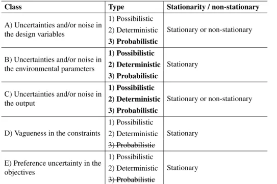
Five sources combined with three types of uncertainties/noise yields theoretically 15 different concepts of uncertainty/noise that can be encountered within optimization problems. When including the distinction between stationary and non-stationary uncertainty/noise and the consideration that multiple types of uncertainties/noise can be present simultaneously within a real-world optimization problem, this picture becomes even more discouraging. Indeed, the variety of cases of uncertainty/noise that can arise from the combinations of the different cases complies with the complexity of real-world scenarios. In practice, however, some scenarios occur more often than others, and those are worthwhile studying in relative isolation (i.e., one type of noise within one part of the optimization model). Table 3.2 summarizes the combinations of class/type of uncertainty/noise as they can occur within optimization problems.

Class Type Stationarity / non-stationary

A) Uncertainties and/or noise in the design variables

1) Possibilistic

Stationary or non-stationary 2) Deterministic

3) Probabilistic

B) Uncertainties and/or noise in the environmental parameters

1) Possibilistic

Stationary

2) Deterministic

3) Probabilistic

C) Uncertainties and/or noise in the output

1) Possibilistic

Stationary or non-stationary

2) Deterministic

3) Probabilistic

D) Vagueness in the constraints

1) Possibilistic

Stationary 2) Deterministic

3) Probabilistic E) Preference uncertainty in the

objectives

1) Possibilistic

Stationary 2) Deterministic

3) Probabilistic

Table 3.2: Classification and categorization of different manifestations of uncertainty/noise as they can

occur within optimization problems. Note that the bold types of uncertainty are considered to be “more common” and the crossed-out types are consdered to be nonexistent.

characteristics for all candidate solutions.

In class B, all three types can be encountered. Uncertainties of probabilistic nature occur when system parameters are due to fluctuations. Possibilistic and deterministic uncertainty occur when model parameters that represent real-world parameters are unknown. Class B uncertainties are always stationary with respect to the given design variables. That is, being fluctuations in the operation conditions of the system, they cannot depend on the particular settings of the design variables.

3.2 Robust Optimization

Up to now, we have discussed the various ways in which uncertainty and noise can present themselves within optimization problems. Given this taxonomy, the next question is: what is robust optimization? In Section 1.1 it is noted that there exist different views on this matter. Some consider robust optimization to involve input uncertainties and/or noise in the design variables (e.g., [BBC11, BNT10]), whereas others consider a broader view, considering robustness with respect to uncertainties within the system or (simulation) model (e.g., [BS07]). In this work, we consider robust optimization to be the practice of optimization given un-certainties and/or noise in the system or (simulation) model. Note that we exclude modeling uncertainty. For any kind of uncertainty and/or noise of class A, B, or C, robust optimization deals with the questions:

• In what way do uncertainties and/or noise within the system or (simulation) model affect optimization algorithms and the practical applicability of solutions found by optimization algorithms?

• How should optimization algorithms be adapted in order to account for uncertainties and/or noise within the system or (simulation) model?

With this we can extend the practical goal of optimization of Definition 2.2.1 and formulate the general goal of robust optimization as:

Definition 3.2.1(Practical Goal of Robust Optimization):Given an optimization problem with

uncertainty and/or noise within the system or (simulation) model, and given an optimization goal and a limited number of resources. Thepractical goal of robust optimizationis to use these resources to find (an) as good as possible solution(s) despite uncertainty and/or noise, that are also optimal and useful in the face of the uncertainties/noise.

Note here that optimality with respect to the uncertainties and/or noise should be defined within the scope of the uncertainty and/or noise at hand. Besides that, from this formal definition two intrinsically different targets of robust optimization can be distinguished, related to uncertainty and noise within optimization problems:

1. Target to find optimal solutions in noisy/uncertain environments. 2. Target to find robust solutions.

Robust Optimization Target Uncertainty class

Finding robust solutions A) Uncertainties and/or noise in the design variables B) Uncertainties and/or noise in the environmental parameters

Optimization in noisy and uncer-tain environments

C) Uncertainties and/or noise in the output

Table 3.3: The two targets of optimization can roughly be related to the place in which the

uncertainty/noise emerges.

emerges when instead of the real-world system, models are used for optimization and candidate solutions or internal model parameters cannot be guaranteed to be set infinitely precise in the real-world system. Hence, it focuses on the robustness of the solutions themselves. Table 3.3 summarizes this global categorization of robust optimization problems.

In literature often isolated scenarios for robust optimization are considered. That is, isolated in the sense that only one particular type of noise/uncertainty, present in one particular part of the system or (simulation) model is considered. The most prominent scenarios are:

• Optimization of noisy objective functions (e.g., [FG88, Bey00])

• Optimization of uncertain objective functions (e.g., [KAE+_09])

• Optimization on systems in which the design variables are affected by uncontrollable and unmeasurable perturbations (e.g., [BOS03])

• Finding robust optima in anticipation of perturbations of the design variables (e.g., [TG97, GA05, ONL06, PBJ06])

• Finding robust optima in anticipation of fluctuations of the environmental parameters (e.g., [Hop09])

• Finding robust optima in anticipation of different operation conditions of the environ-mental parameters (e.g., [RKD+_11])

3.3 Real-World Robust Optimization Scenarios

This section is devoted to present three real-world optimization scenarios in which uncertainty and noise are inherent parts of the system of interest. These scenarios are related to the view on robust optimization as presented in this chapter.

3.3.1 Deep Drawing Optimization

The optimization of the design of a deep drawing process for sheet metal forming in engin-eering is a typical example of a robust optimization problem (see, e.g., [SH04, PLBG07]). The design of a deep drawing process involves finding proper settings for the process (e.g., drawing forces), such that the end product of the deep drawing process is of the desired geometrical shape that complies to, or is as good as possible with respect to properties relating to plasticity, thickness, and probability of forming failure. In practice, finite element software is often used for virtual testing of candidate designs. Hence, the design of a deep drawing process is an optimization problem for which automated optimization techniques are in principle well-suited. Uncertainty and noise arise in several ways in such optimization problems:

A) Uncertainties and/or noise in the design variables:

In the real-world manufacturing process, the drawing forces, such as the drawbead forces, the binder force, and the punch force cannot be set infinitely accurately (type 3). Designs should be robust against fluctuations in these variables.

B) Uncertainties and/or noise in the environmental parameters:

Parameters within the simulation model are uncertain and/or noisy, e.g., the friction coefficient (type 1/2) or the blank thickness (type 3). Designs should be robust against these uncertainties and fluctuations.

C) Uncertainties and/or noise in the output:

Due to the limited accuracy of a (finite element) simulator, the simulation output is not guaranteed to match real-world behavior exactly (type 1/2). The optimization algorithm should be robust against this type of uncertainty and find good solutions despite the difficulty in the quality assessment of candidate designs.

The robust optimization goals for such problems are to find optimal designs (or solutions) that are robust against fluctuations and uncertain conditions in real-world practice, and furthermore to assure robustness of the optimization process itself, that has to deal with the uncertainty in the assessment of the quality of candidate solutions.

3.3.2 Building Performance Optimization

[HHPW07, EHM+08, Hop09, HTHB11]. Consider, for example, the problem of optimizing building designs for thermal comfort (maximization) and energy consumption (minimization) with respect to the following design variables: infiltration rate (air exchange rate per hour in the building), window fraction (the amount of glass percentage on one wall of the building), load equipment (power equipment per net floor surface), and load lighting (power lighting per net floor surface). By using BSP tools for the evaluation of candidate solutions (i.e., alternative designs), automated optimization can be used to optimize building designs. The ways in which uncertainty and noise arise in such optimization problems are:

B) Uncertainties and/or noise in the environmental parameters:

The operation conditions of a building in the real-world are uncertain and fluctuating. An obvious example is the outside temperature that changes from hour to hour and from day to day. For successful integration of optimization in this context, candidate designs should be evaluated with respect to these fluctuating environmental operating conditions.

C) Uncertainties and/or noise in the output:

BPS tools are not guaranteed to match the real-world behavior exactly (type 1/2). The optimization algorithm should be able to find high quality designs despite the difficulty in the quality assessment.

Moreover, although we do not consider them in the scope of robust optimization, also uncer-tainties of class E emerge in such problems. That is, thermal comfort is a typical objective in which preference uncertainty arises as this is an inherently subjective objective, these indicators are fuzzy measures.

3.3.3 Molecular Design Optimization

Inde novodesign of molecular structures, the challenge is to find molecular structures that

could be active components of drugs. In order for a molecular structure (or ligand) to be suitable as a drug component, a number of criteria should be met. First, it should be active on the targeted receptor. Second, it should fulfill a number of criteria such that it is actually taken in by the body, it is not toxic or harmful in other ways, and it should be possible to actually create (synthesize) the structure (preferably as easily as possible).

In practice, automated methods can be used forin silico design of candidate molecular structures (see, e.g., [NAP09, KBIvdH08, KAE+_{09]). A simple setup, for instance, is to use}

C) Uncertainties and/or noise in the output:

The simulation output of the docking simulator is an approximation of the real-world behavior (type 1/2). Due to the use of a stochastic simulator, the outputs of the simulator are noisy (type 3). The optimization algorithm should be robust against these types of uncertainties and noise and find good solutions despite the difficulty in the quality assessment of candidate molecular structures.

Moreover, although we do not note them as being in the scope of robust optimization, also uncertainties of class D and class E emerge in such problems. Vagueness in the constraints can emerge when constraint bounds are used for the simple descriptors that determine the likelihood of a candidate ligand to be generally suitable as a drug (see, e.g., [KEB+_09b]).

Preference uncertainty can emerge when the objectives are combined into one aggregate scoring function.

3.4 Summary and Discussion

In this chapter we have extended the model of optimization problems as presented in Chapter 2 to a model that includes uncertainties and noise as they can arise in real-world optimization problems. It has been shown that the various sources and types of uncertainty and noise yield a combinatorial explosion of different scenarios. Yet, a few isolated scenarios can be identified that emerge frequently, hence, are worthwhile subjects of study.

In this work, we consider robust optimization as the practice of optimization given un-certainties and/or noise in the system or (simulation) model. Hence, we exclude unun-certainties that arise from the modeling of an optimization problem. Robust optimization deals with two goals: 1) the aim to find optimal solutions in noisy/uncertain environments, and 2) the aim to find robust solutions.

The concepts introduced in this chapter were exemplified by means of three real-world optimization scenarios; deep drawing optimization, building performance optimization, and molecular design optimization. For these three scenarios it was illustrated how the various forms of uncertainties/noise enter the optimization model, therewith stressing the importance of robust optimization.