Allocating the Sample Size in Phase II and
III Trials to Optimize Success Probability
(Resource Allocation to Optimize Success)
Daniele De Martini(1)
Background: clinical trials of phase II and III often fail due to poor experimental planning. Here, the problem of allocating available resources, in terms of sample size, to phase II and phase III is studied with the aim to increase the success rate. The overall success probability (oSP) is accounted for. MeTHodS: Focus is placed on the amount of resources that should be provided to phase II and III trials to attain a good level of oSP, and on how many of these resources should be allocated to phase II to optimize oSP. It is assumed that phase II data are not considered for conrmatory purposes and are used for planning phase III through sample size estimation. Being r the rate of resources allocated to phase II, oSP(r) is a concave function and there is an optimal allocation ropt giving max(OSP). If MI is the sample size giving the desired power to phase III, and kMI is the whole sample size that can be allocated to the two phases, how large k and r should be is indicated in order to achieve levels of oSP of practical interest.
reSulTS: For example, when 5 doses are evaluated in phase II and 2 parallel phase III conrmatory trials (one-tail type I error = 2:5%, power = 90%) are considered with 2 groups each, k = 24 is needed to obtain oSP ≃ 75%, with ropt≃ 50%. The choice of k depends mainly on how many phase II treatment groups are considered, not on the eect size of the selected dose. When k is large enough, ropt is close to 50%. an r ≃ 25%, although not best, might give a good oSP and an invitingly small total sample size, provided that k is large enough.
concluSIonS: To improve the success rate of phase II and phase III trials, the drug development could be looked at in its entirety. resources larger than those usually employed should be allocated to phase II to increase oSP. Phase II allocation rate may be increased to, at least, 25%, provided that a sucient global amount of resources is available.
Key words: overall success probability; allocation rate; launching rules; sample size estimation; optimal allocation; sucient resources.
(1) Dipartimento DiSMeQ - Universita degli Studi di Milano-Bicocca
Corresponding author: Daniele De Martini- Dipartimento DiSMeQ - Universita degli Studi di Milano-Bicocca - Via Milano-Bicocca degli Arcimboldi 8, 20126 Milano - Italia - E-mail: [email protected]
Tel.+39-02-6448-3130
doi: 10.2427/9958
1
Introduction
It is common knowledge that the aim of phase II clinical trials is mainly
exploratory, while that of phase III is confirmatory, and that phase II also serves to enhance planning for the subsequent phase III. Usually, phase II is small with respect to phase III, and the rate of trial failures, which is around 60% and 40% for phase II and III respectively suggests that this habit might not be helpful. In general, low success probabilities are often due to low sample size [1]. Here, we study sample size problems from the perspective of a drug development project, which means considering jointly phase II and phase III sample sizes.
To introduce the problem, by way of example, let us suppose that a phase II trial has been run, with 2 parallel arms each with 60 patients, and that a phase III with the same design needs to be planned. Assume that the efficacy value (standardized effect size) of minimum interest that should be observed to then launch phase III is 0.15 and that a value slightly higher than this has been observed in phase II, so that phase III has to be launched. With one-sided α= 2.5% and power 1−β= 90%, approximately 940 patients should be recruited for each group, if the observed effect size is adopted for sample size computation - namely pointwise strategy [2, 3]. This number (940) is quite high, but not beyond the range of those usually adopted in phase III trials (visit clinicaltrials.gov, a service of the U.S. NIH). So, assuming that the research team decided to actually launch phase III, the total number of patients enrolled in about 2,000.
Now, the point is: if the resources for studying 2,000 patients were actually available, would there be an allocation of sample size better than 60/940? Would, for example, 400 data allocated to phase II and, at most, 600 to phase III has been a better choice? It is worth noting that we wrote at mostbecause when 400 data per group come from phase II and are used for estimating the phase III sample size, this is not necessarily 600, where it is almost surely lower. Moreover, what does “better allocation” mean? And, is there an optimal allocation?
Besides dose selection and safety evaluation, the aims of phase II are to correctly decide go/no-go, to launch phase III (i.e. go) with a high probability if a
providing the desired probability of success of phase III); the aim of phase III is to prove efficacy with a high probability, once again if a meaningful effect really exists. Hence, the aim is to succeed with high probability in both phases, whenever the drug under study actually works well.
In this paper we study sample size resource allocation in terms of overall
probability of success (OSP): we focus on the amount of resources that should be provided to phase II and III trials so as to attain a good level of OSP, and on how many of these resources should be allocated to phase II to optimize OSP. Since not all the resources allocated to phase III are spent, depending on sample size
estimation, we also focus on the actual amount of resources used. It is assumed that phase II data provide information for phase III planning and are not used for phase III confirmatory analysis.
Analogous computations on success probability have recently been proposed by Jiang [4] under the Bayesian framework. Here, the frequentist approach is adopted: this is due to poor performances of Bayesian sample size estimators (proposed, for example, by Chuang-Stein [5]) in terms of high variability of their results [3].
2
Theoretical framework
2.1 Drug development model
It is assumed that a certain disease is under study, and that hdoses of a new drug for the disease of interest are evaluated in a phase II trial (hoften varies from 3 to 7). Also, a placebo arm is run. A classical parallel design is applied in the
exploratory phase II, with h+ 1 groups. If phase II results are promising, a single dose D is chosen and 2 phase III trials comparing to placebo are run, once again
under parallel design. It is also assumed that the three trials (1 phase II and 2 phase III) share the same response variable and the same patient population, meaning that the effect size of the elected dose is the same in both phases. These assumptions allow simple sample size estimation, with no need for further
where h= 1 and only one phase III trial were considered. Here, all trials are run under balanced sampling.
A certain limited amount of resources is available to develop phase II and III trials, and this translates into a total of at most w patients. Let r∈(0,1) be the rate of w allocated to phase II: if a sample of size n is studied for each treatment in phase II, then n is, approximately, rw/(h+ 1). Consequently, the whole sample size available for phase III is w(1−r), which is not used entirely (almost surely).
Indeed, the phase III sample size actually adopted for each group (Mn) is
estimated on the basis of phase II data and is a random variable whose maximum is w(1−r)/4 (4 are phase III groups).
2.2 Phase II tools
Let δ= (µD−µP)/σ be the generic standardized effect size, µD and µP the means of response variables of the populations under D and under placebo. Without loss of
generality σ= 1. The true, unknown, effect size is δt. X¯D,n and X¯P,n are the means of measurements and dn = ¯XD,n−X¯P,n is the pointwise estimator ofδt.
Call L the random event representing the success of phase II -L stands for phase III launch. L can be defined in some different ways: for example, on the basis of the maximum sample size mmax for phase III (i.e. L ⇔Mn≤mmax), or the basis of the
observed effect size overcoming a threshold of clinical relevance (i.e. L ⇔dn> δ0L). Kirby et al.[7] evaluated some further launching rules, which, through simple algebra, can be reduced to L ⇔dn> δ0L, for some values ofδ0L. Note that the first two launching criteria above can be set to result mathematically equivalent ([1], Ch.3).
Although the launching rule based on δ0L is the most intuitive, and one of the most used, let us adopt the one pragmatically based on mmax. In this framework
constrained by w and modeled by r, the actual launching rule becomes
Mn≤mmax(r) = min{mmax, w(1−r)/4}. For completeness,Mn≤mmax(r)translates into
L ⇔dn> δ0L(r) = max{δ0L,2(z1−α+z1−β)
Phase II success probability is:
SPII(r) =Pδt(L) =Pδt(dn> δ0L(r)) =Pδt(Mn≤mmax(r))
2.3 Phase III tools
The Z-test is adopted with one-sided alternatives. Beingm the generic sample size,
Tm=m/2( ¯XD,m−XP,m¯ ) is the test statistic and the success probability, according
to [1], Ch.3, is Pδt(Tm> z1−α) =SP(m).
1−β is the desired power to be achieved in each phase III trial (e.g. 90%); then, the
ideal sample size per group for each phase III trial is:
MI = min{m|SP(m)>1−β}=2(z1−α+z1−β)2/δ2t+ 1 (1)
Once phase II has succeeded, phase III is run with the sample size estimated by the 2n phase II data. Several sample size estimation strategies can be adopted [1].
Here, MI is estimated by the pointwise estimator based on the observed effect size dn:
Mn=2(z1−α+z1−β)2/d2n+ 1 (2)
The adoption of the pointwise strategy is made for simplicity and also because its performances in terms of OSP and MSE are acceptable although not best [3]. Two confirmative phase III trials are run simultaneously and independently, each group with Mn patients, so that the success probability is the random variable (SP(Mn))2. The mean of(SP(Mn))2, conditional to L, is of main interest and,
although it has been called Average Power by Wang et al.[2], we call it the SP of phase III:
SPIII(r) =
mmax(r)
m=2
(SP(m))2Pδt(Mn=m|L) (3)
2.4 Defining OSP
the analysis of phase III data, OSP is given by the product of the success probabilities of phases II and III:
OSP(r) =SPII(r)×SPIII(r) =
mmax(r)
m=2
(SP(m))2Pδt(Mn=m) (4)
We expect OSP(r)to be low for small values of r, due to a low launch probability
(i.e. SPII(r)). Also, OSP(r) is expected to be low for high values of r, due to low
values of SPIII(Mn)since Mn is limited by a low value mmax(r). Then, there is an intermediate allocation of resources that optimizes OSP(r), that is
ropt=argmax{OSP(r)}.
3
Behavior of OSP
3.1 Settings
It has recently been shown [3, 7], that the threshold of clinical relevance δ0L should be set not too close to δt, in order not to penalizeSPII. A threshold aroundδt/3 is therefore set, accordingly. Phase III type I error is 2.5%, where the power is
1−β= 90% (according to [2, 3]). Three effect size values are considered
(δt= 0.2,0.5,0.8), providing ideal phase III sample size MIs resulting 526,85,33, from (??). For each δt, the whole sample sizew is taken equal to kMI, with
k= 10,15,20,25,30. Three numbers of doses hare accounted for: 3,5,7. For each of
the 45settings (3 δts ×5 ks ×3 hs),r is considered varying from 5% to95%.
3.2 Simplifying launching rule
Let us translate the launch threshold based on the effect size into that based on the maximum sample size, and then simplify OSP formulas. Being δ0L=δt/3, we have mmax=2(z1−α+z1−β)2/(δt/3)2+ 19MI. For all 45settings, the maximum
sample size introduced by the constraint of available resources, i.e. w(1−r)/4, results lower than 9MI. Consequently, mmax(r)turns out to be w(1−r)/4. The OSP in equations (??) is computed by replacing mmax(r) with w(1−r)/4. The actual launching threshold for the effect size becomes δ0L(r) = 2(z1−α+z1−β)2/w(1−r),
90 80 70 60 50 40 30 20 10 1.2
1.0
0.8
0.6
0.4
0.2
0.0
r (%)
d
e
lt
a
_0L
0.17
10 15 20 25 30 k
Launch thresholds delta_0L vs r (%)
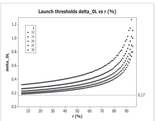
Figure 1: Launch thresholds δ0L, obtained with α = 2.5%, 1−β = 90%, δt = 0.5, and with
k= 10,15,20,25,30.
based on the constraint on sample size given by the available resources are stricter than δt/3 (see Figure ??, where δ0L(r) as a function of ris reported - varying δts and
hs the curves result very similar). Hence, if δt/3 is considered a threshold of clinical
relevance, a fortiori2(z1−α+z1−β)
2/w(1−r) is so.
Note that this stricter launching rule penalizing the probability of launching phase III (i.e. SPII) is imposed by the model we are studying.
3.3 Computing OSP
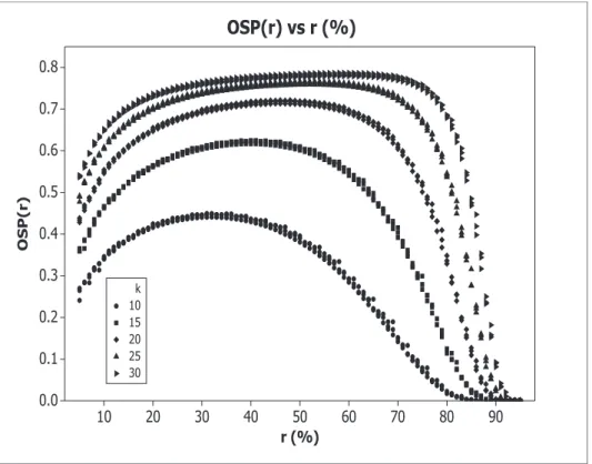
OSP functions, with h= 5, are reported in Figure??: OSP(r) under different δts are very similar - they lie approximately on the same curves.
at least 20(see Figure ??). When k= 10,15, we have max{OSP}=OSP(ropt)45%,
and max{OSP} 63%, respectively. With k= 20, max{OSP} 72% - the optimal rates ropts under different δs are very close (i.e. ropt47%). For k= 25,30, we have
max{OSP} 76%,78%, withropt52%,60%, respectively.
90 80 70 60 50 40 30 20 10 0.8
0.7
0.6
0.5
0.4
0.3
0.2
0.1
0.0
r (%)
OS
P
(r
)
10 15 20 25 30 k
OSP(r) vs r (%)
Figure 2: OSP(r), obtained with α = 2.5%, 1−β = 90%, h = 5, δt = 0.2,0.5,0.8, and with
k= 10,15,20,25,30.
For k≥20,OSP(r) shows a quite flat shape around its maximumropt, meaning that
even if the rater allocated to phase II is a bit smaller than ropt,OSP(r) still
provides acceptable values. For example,OSP(30%)70%,74%,76%, with k= 20,25,30, respectively.
Finally, ropt moves from 34% to 60% with k increasing from10 to 30: whenw
increases, the best solution is to allocate more and more sample size to phase II, to improve both SPII and the precision in estimating MI.
90 80 70 60 50 40 30 20 10 0.8
0.7
0.6
0.5
0.4
0.3
0.2
0.1
0.0
r (%)
OS
P
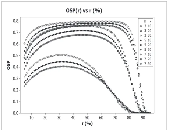
3 10 3 20 3 30 5 10 5 20 5 30 7 10 7 20 7 30 h k OSP(r) vs r (%)
Figure 3: OSP(r), obtained with α = 2.5%, 1−β = 90%, h = 3,5,7, δt = 0.5, and with
k= 10,20,30.
(even higher if h= 7) is suggested to reach suitable OSP values.
4
Sizing the whole amount of resources
Since the desired SPIII is (90%)2= 81%, and a goodSPII level may be still around
90% - we remind that the aim is to study how to increase the success rates in
clinical trials, we consider OSP around 72% as acceptable.
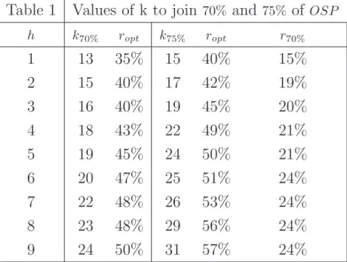
In Table 1, the values of k providing a maximum OSP of at least 70%,75% (viz.
k70%, k75%), are given, together with ropt, with hfrom 1 to 9. Moreover, whenk75%s
are computed, also the smallest r giving an OSP at least 70% is given (viz.
The total amount of resources needed to reachOSP = 70% is, withh= 3,5,7,
w= 16MI,19MI,22MI, respectively, with ropt= 40%,45%,48%. If smaller rs are
allocated to phase II, OSP falls below70% (e.g. OSP(20%)64%).
When the75% level is adopted, higher ks are needed: withh= 3,5,7,k= 19,24,26,
respectively, provide the required OSP with ropt= 45%,50%,53%. However, if smaller
rs are adopted, acceptable OSP levels are still provided: rs around 20% give
OSP(r)70%.
Table 1 Values of k to join70% and 75% of OSP
h k70% ropt k75% ropt r70%
1 13 35% 15 40% 15%
2 15 40% 17 42% 19%
3 16 40% 19 45% 20%
4 18 43% 22 49% 21%
5 19 45% 24 50% 21%
6 20 47% 25 51% 24%
7 22 48% 26 53% 24%
8 23 48% 29 56% 24%
9 24 50% 31 57% 24%
Table 1. Minimum values of k to join a max OSP of at least 70%,75% (viz.
k70%, k75%), withα= 0.025, 1−β = 0.9,h= 1, . . . ,9, and δt= 0.5, together with the
allocationsropt providing max of OSP. Moreover, r70% indicates the smallest
allocation providing OSP at least 70%, when k75% is adopted.
As a rule of thumb, in order to obtain an OSP 75%, with a number of phase II
groups ranging from2 to10 (and 2 phase III confirmatory trials) provide to the
whole development project sufficient resources to recruit a number of patients from
15to 30 times (increasing linearly withh) the ideal sample size MI, and allocate
about 50% of the sample size to phase II, regardless of the amplitude of δt.
Moreover, if just20% of resources is allocated to phase II,OSP remains near70%,
provided that resources to reachOSP = 75% are stored before starting phase II.
We remark that not all the stored resources are used: rw is actually spent in phase
4.1 Assuring the whole amount of resources
The problem that in practice δt is unknown does not influence the allocation choice
based on OSP, since OSP(r)is almost independent of δt. Nevertheless, to allocate
enough resources to obtain a given OSP level, depends on δt. In particular, since
we adopted MI as a unit measure forw, the resources needed depends on δt
through MI.
In practice, the unknown MI should be replaced by
Ma=M(δa) =2(z1−α+z1−β)2/δa2+ 1, whereδa is the assumed effect size. However,
how close Ma is to MI is unknown. To reinforce the assumption onδa and limit the
uncertainty of parameter, assurance can be applied [9]. This consists in defining a distribution around δa (viz. fδa(t)) so that the assured sample size becomes
MA= M(t)fδa(t)dt - it can be viewed as Bayesian sample size determination,
where fδa(t) plays the role of the prior distribution.
For example, when the uniform prior fδa(t) = 1/(2δa), t∈(δa/2,3δa/2), is adopted, we find MA= 4Ma/3.
The linear rule of thumb above, through assurance, suggests providing the whole development project when h= 5 with sufficient resources to recruit 22.5MA patients,
i.e. 22.5×4/3 = 30 times the assumed sample size Ma. A lower assurance provides 22.5≤k≤30.
5
Mean and variability of total sample size
An indispensable aspect of this sample size allocation problem is to evaluate the actual amount of resources spent in phase III, as well as those spent overall, depending on the behavior of the sample size estimator Mn.
Mn is a random variable that for smallrs, i.e. when n is low, might be imprecise:
the average and the MSE (measuring variability) of Mn, conditional to phase III
launch, are:
E[Mn|L] = mmax(r)
m=2
m Pδt(Mn =m|L)
M SE[Mn|L] = mmax(r)
m=2
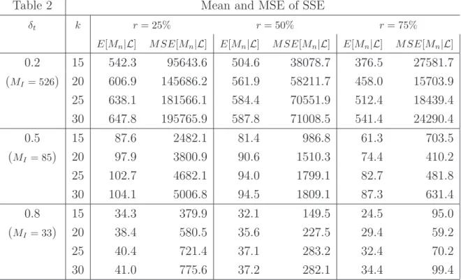
Table 2 Mean and MSE of SSE
δt k r= 25% r= 50% r= 75%
E[Mn|L] M SE[Mn|L] E[Mn|L] M SE[Mn|L] E[Mn|L] M SE[Mn|L]
0.2 15 542.3 95643.6 504.6 38078.7 376.5 27581.7
(MI = 526) 20 606.9 145686.2 561.9 58211.7 458.0 15703.9
25 638.1 181566.1 584.4 70551.9 512.4 18439.4 30 647.8 195765.9 587.8 71008.5 541.4 24290.4
0.5 15 87.6 2482.1 81.4 986.8 61.3 703.5
(MI = 85) 20 97.9 3800.9 90.6 1510.3 74.4 410.2
25 102.7 4682.1 94.0 1799.1 82.7 481.8
30 104.1 5006.8 94.5 1809.1 87.3 631.4
0.8 15 34.3 379.9 32.1 149.5 24.5 95.0
(MI = 33) 20 38.4 580.5 35.6 227.5 29.4 59.2
25 40.4 721.4 37.1 283.2 32.4 70.2
30 41.0 775.6 37.2 282.1 34.4 99.4
Table 2. Mean and MSE ofMn, with α= 0.025, 1−β= 0.9, h= 5, δt= 0.2,0.5,0.8,
k= 15,20,25,30and r= 25%,50%,75%.
In Table 2, the average and the MSE are shown withk= 15,20,25,30, h= 5, and with r= 25%,50%,75%. When k increases and r is fixed, both mean and MSE of
Mn|L increase. Mainly, the estimation process becomes more reliable whenr
increases: the mean of Mn|L tends toMI and MSE decreases.
Moreover, whenk= 25and r= 50% (viz. operating conditions giving high OSP when h= 5), the mean ofMn is close to MI and the mean error is about MI/2, for
every δt. Indeed, the behavior ofMn is almost independent of δt, in accordance
with that of OSP.
Now, let us consider how these numbers reflect on the whole amount of resources spent in both phases, viz. on the total sample sizeMT =MI×k×r+ 4Mn. From a
practical standpoint, the settings withk= 20,25 and r= 25%,50% are the most interesting - k= 30 providesOSP higher than requested, and with k= 15the OSP is often low; also, OSP is low withr= 75%, due to strict constraints forMn.
When k= 25 and r= 50%, and with δt= 0.5 giving MI = 85, the average amount of
deviation of σ(MT)2MI - recall, this is almost independent of δt. Percentiles for
Mn, and so for MT, can be obtained through conditional probability calculation: for example, with δt= 0.5 and under the latter setting (i.e.
n= 25×85×50%/(5 + 1)177), the 80% and 90% percentiles are m.8
177= 122 and
m.9
177= 151. Once again, percentiles present small variations in function of δt.
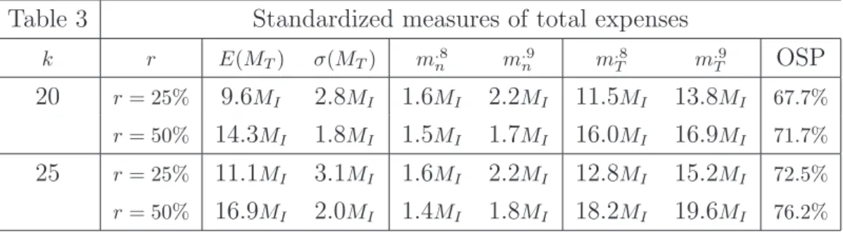
Mean, standard deviation and percentiles of MT for the four settings considered of main interest are reported in Table 3. In the light of these further results, even allocation rs that do not provide optimal OSP may be of practical interest. For example, when k= 25 is adopted (i.e., w= 25MI is stored) andr= 25% of resources are allocated to phase II, the average of MT is 11.1MI and MT does not overcome
12.8MI with 80% probability, where OSP(25%) = 72.5%.
Table 3 Standardized measures of total expenses
k r E(MT) σ(MT) mn.8 m.n9 m.T8 m.T9 OSP
20 r= 25% 9.6MI 2.8MI 1.6MI 2.2MI 11.5MI 13.8MI 67.7%
r= 50% 14.3MI 1.8MI 1.5MI 1.7MI 16.0MI 16.9MI 71.7%
25 r= 25% 11.1MI 3.1MI 1.6MI 2.2MI 12.8MI 15.2MI 72.5%
r= 50% 16.9MI 2.0MI 1.4MI 1.8MI 18.2MI 19.6MI 76.2%
Table 3. Standardized mean, st.dev. and percentiles of the total expenses in terms of sample size (viz. MT), through percentiles ofMn, obtained with α= 0.025,
1−β= 0.9, h= 5, k= 20,25and r= 25%,50%; δt= 0.5 has been adopted.
6
Example
Let’s continue the introductory example, where the sample size of each phase II group was n= 60. Assume here thath= 7 doses are studied in phase II, and that two phase III trials are launched if d60> δ0L= 0.15. Settingα= 2.5%and 1−β= 90%,
if δt= 0.4 then MI = 132; also, mmax= 940. Note that if δt was 0.4, to obtain an
observed value of d60 near 0.15, and so a phase III sample size estimate close to 940, is not a low probability event, since 0.15 is approximately the 8.5th percentile of
d60∼N(0.4,2/60).
= 25, in accordance with Table 1, so that resources for treating a total of
25×132 = 3300 patients are available for the allocation into the two phases. Then,
things go better: with r from 29% to 68% the OSP is higher than 70%. In detail,
max{OSP}= 73.5%with r= 51%, where the SP of phase III (also called Average
Power) is 76.4% and the launch probability is 96.2%.
This best r= 51% gives n= 211 (i.e. 1688patients to be enrolled in phase II) and a maximum phase III sample size, per group, of 403. Actual values of phase III sample size result often lower than 403: the average of M211 is 146.85, and its standard deviation is 69.74. Consequently, the average and the standard deviation of the total sample size MT are 2276 and 279. This corresponds to, about,17.2MI and 2.1MI, respectively, meaning that not all the w= 25MI resources would be spent.
7
Discussion
Although the development of a drug, and in particular the clinical part regarding phase II and III trials, might be looked at in its entirety, scientists and trial managers often tend to focus on each phase separately. In particular, resources to develop the research project are often funded for each phase separately. It is a fact that the failure rate of phase II and phase III clinical trials is quite high.
Here, the assumption is that the whole amount of resources to develop phase II and III trials (in terms of sample size) is stored, and therefore potentially available before starting phase II. We studied the problem of allocating the resources to the two phases - to be precise, resources allocated to phase II are all used, where those used in phase III are at most those left, depending on phase III sample size
estimation based on phase II data.
It was assumed that 2 phase III trials are run with a sample size estimated on the basis of phase II data. The overall success probability (OSP) has been evaluated as a tool for planning experiments, in accordance with some recent papers [8, 4, 3], and the variability of the resources actually spent has been accounted for.
ALLOCATING THE SAmPLE SIzE IN PHASE II ANd III TRIALS TO OPTImIzE SuCCESS PROBABILITy
of the dose selected in phase II. Moreover, to obtain the optimal OSP, the rate of resources to be allocated to phase II is often close to 50%. Even an amount of
resources of 25% might give a good OSP and an invitingly small total sample size if allocated to phase II, provided that a sufficient amount of resources is stored to the two phases. If the whole amount of resources available for the two phases is low, the OSP will be low too, even lower than 50%, even if the best allocation of resources is made. SinceMI depends on the unknown effect size of the selected dose, wrong assumptions regarding the latter can cause too small investments and low OSP. To reduce this risk,MI may be computed by applying assurance [9] on effect size assumptions.
The observed phase II effect size was adopted to compute phase III sample size: being aware of the variability in effect size estimation, conservative sample size estimation strategies may be adopted, as in [1]. The OSP can, therefore, result in a considerable increase (i.e. about 3%when OSP 75% - unpublished result). Allocations near50% providing the optimal OSP are usually not adopted in clinical practice: phase II often absorbs less resources than phase III. Indeed, the size of samples adopted in phase II is, on average, 10–15% of the total sample size of the two phases [1]. To improve the success rate of phase II and phase III trials, the drug development could be looked at in its entirety, and phase II allocation might be increased to, at least, 25%, provided that a sufficient global amount of resources is available. Then, a more accurate phase II would also induce a higher probability of choosing the best dose among those considered. Nevertheless, larger phase II trials imply higher costs and longer times for the development project, allowing for a shorter patent life and so lower potential profits, of course in case of successful trials. Allocation of resources should also be evaluated from an economic
perspective, as suggested also by Jiang [4]. For this reason, our future works may focus on the relationship among allocations, OSP, efficacy and safety utility functions, costs, revenues, and profits, according to [10, 11].
The indications on the amount of resources to be allocated to phase II suggested by Jiang [4] differ from ours, but in that paper only 2 phase II groups and 1 phase III trial are taken into account. Differences between our indications and those provided by Stallard [12] are much more evident, since phase II data are
considered only for detecting a certain effect with low power, not for adequately
16
planning phase III.
references
[1] De Martini D. Success Probability Estimation with Applications to Clinical Trials. John Wiley & Sons: Hoboken, NJ, 2013.
[2] Wang SJ, Hung HMJ, O'Neill RT. Adapting the sample size planning of a phase III trial based on phase II data. Pharmaceutical Statistics 2006; 5: 85-97. [3] De Martini D. Adapting by calibration the sample
size of a phase III trial on the basis of phase II data. Pharmaceutical Statistics 2011; 10 (2): 89-95. [4] Jiang K. Optimal Sample Sizes and Go/No-Go
Decisions for Phase II/III Development Programs Based on Probability of Success. Statistics in Biopharmaceutical Rerearch 2011; 3: 463-475. [5] Chuang-Stein C. Sample Size and the Probability of
a Successful Trial. Pharmaceutical Statistics 2006; 5: 305-309.
[6] De Martini D. Robustness and corrections for sample size adaptation strategies based on eect size estima-tion. Communications in Statistics - Simulation and Computation 2011; 40 (9): 1263-1277.
[7] Kirby S, Burke J, Chuang-Stein C, Sin C. Discounting
phase 2 results when planning phase 3 clinical trials. Pharmaceutical Statistics 2012; 11, 5: 373-385. [8] Fay MP, Halloran ME, Follmann DA. Accounting
for Variability in Sample Size Estimation with Applications to Nonhaderence and Estimation of Variance and Eect Size. Biometrics 2007; 63: 465-474. [9] O'Hagan A, Stevens JW, Campbell MJ. Assurance in
clinical trial design. Pharmaceutical Statistics 2005; 4: 187-201.
[10] Patel N., Bolognese J., Chuang-Stein C., Hewitt D., Gammaitoni A., Pinheiro J. Designing Phase 2 Trials Based on Program-Level Considerations: A Case Study for Neuropathic Pain. Drug Information Journal 2012; 46, 4: 439-454.
[11] Chen MH., Willian AR. Determining optimal sample size for multistage adaptive randomized clinical trials from an industry perspective using value of informa-tion methods. Clinical Trails 2013; 10: 54-62