ISSN 2307-7743 http://scienceasia.asia
THE HALF LOGISTIC-POISSON DISTRIBUTION
MUSTAPHA MUHAMMAD∗ AND MARYAM A. YAHAYA
Abstract. In this article, a new two-parameter distribution called the half Logistic Pois-son distribution is proposed. Numerous properties of the new distribution are discussed,
maximum likelihood estimation procedure is considered for parameter estimation; we also assessed the maximum likelihood estimators by a simulation study. Application of the new
distribution to a real data set is provided for illustration purposes.
1. Introduction
Distributions with support on the positive real line are widely used in modeling of lifetime data in practical applications. For example, exponential and Weibull distributions have been used in fitting data set in various fields of science and applied sciences such as in the fields of biomedical studies, reliability, actuarial sciences, demography, engineering, public health, etc. Moreover, half-logistic distribution (HL) is another lifetime model that plays a vital role in fitting data with decreasing failure rate in practice.
In lifetime study we required more distributions with flexibility that can accommodate different kind of data set in practice. In consideration of these kinds of problems, several authors give an important attention to half logistic distribution in recent years and proposed various extensions and new forms of the half-logistic such as the generalized half logistic (GHL), power half logistic (PwHL) by [23], Olapade generalized half logistic (OGHL) by [39], exponentiated half logistic family of distributions (EHL-G) by [11], type I half-logistic family (TIHL-G) by [10] among others.
In this work, the proposed distribution is obtained via compounding the half Logistic and Poisson distributions. The new distribution serves as the complementary distribution to the Poisson-half logistic distribution (PHL) proposed by [1].
There are so many parametric models that have been successfully proposed and investi-gated by combining discrete and continuous distributions, for instance, [2, 24, 46] proposed the exponential geometric (EG), exponential Poisson (EP), BurrXII Poisson (BXIIP) dis-tributions respectively, where their complementary disdis-tributions are the complementary ex-ponential geometric (CEG), Poisson-exex-ponential (PE) and BurrXII-zero-truncated Poisson (BXIIZTP) distributions introduced and studied by [26], [8] and [36] respectively.
Key words and phrases. Half logistic distribution; Moments; Maximum likelihood estimates.
c
Some others include the complementary exponentiated exponential geometric (CEEG), complementary Weibull geometric (CWG), complementary Poisson-Lindley (CPL), comple-mentary exponentiated Inverted Weibull Power Series (CEIWPS), Complecomple-mentary Burr III Poisson (CBIIIP) and complementary extended Weibull power series (CExWPS) distribu-tions proposed by [25,48,17,19,18] and [12] respectively. In the same approach, we have the exponentiated exponential Poisson (EEP) by [42], exponentiated exponential binomial(GEB) by [6], generalized exponential power series (GEPS) by [28], binomial exponential-2 (BE2) by [5], linear failure rate-power series (LFRPS) by [29], Weibull power series(WPS) by [34], extended Weibull power series (EWPS) by [45], exponentiated Weibull-logarithmic (EWL) [27], exponentiated Weibull Poisson (EWP) by [30], Additive Weibull-Geometric by [15], ex-ponentiated Weibull geometric (EWG) by [31], exponentiated Weibull power series (EWPS) by [32], Lindley-Poisson (LP) by [16], Generalized Gompertz-power series (GGPS) by [47], exponentiated BurrXII Poisson (EBXIIP) by [14], modified Weibull geometric (MWG) by [49], Dagum-Poisson (DP) by [40], Poisson-Lomax (PL) by [3], complementary exponentiated BurrXII Poisson (CEBXIIP) by [38], Poisson-odd generalized exponential family (POGE) by [37] and the additive modified Weibull odd Log-logistic-G Poisson family by [33] etc.
The rest of the paper is arranged as follows, the properties of the proposed distribution are derived and discussed in section 2. In section 3, estimation of the unknown parameters by maximum likelihood and simulation results are presented. An application of the HLP is given in section 4. Sections 5 conclude the paper.
2. HLP and Properties
The probability density function and cumulative distribution function of the half Logistic distribution with scale parameter α >0 are defined by
g(x) = 2αe
−αy
(1 +e−αy)2
(1)
and
G(x) = 1−e
−αy
1 +e−αy.
(2)
respectively.
The proposed model, that is the half Logistic Poisson (HLP) distribution is obtained using the procedure followed by [26] and [8], the process is summarized by the followingproposition.
Proposition 2.1. Let X = min{Y1, Y2,· · · , Yk}, where Y1, Y2,· · · , Yk, are independent and
identically distributed half Logistic random variables with ( 1). Let K be a Poisson random variable truncated at zero with probability mass function given by P(k;λ) = λk((exp(λ)−
1) k!)−1, λ > 0 and k ∈
N. Then, the probability density function of X (the half Logistic
The probability density function, cumulative distribution function, survival and hazard rate functions of the half Logistic Poisson with parameters α > 0 and λ ∈ R− {0} are defined by
f(x, α, λ) = 2αλe
−αx
(1−e−λ)(1 +e−αx)2e
−λ1−e−αx
1+e−αx
, (3)
F(x) = 1−e
−λ1−e−αx
1+e−αx
1−e−λ ,
(4)
s(x) = e
−λ1−e−αx
1+e−αx
−e−λ 1−e−λ ,
(5)
h(x) = 2αλe
−αxe−λ
1−e−αx
1+e−αx
(1 +e−αx)2
e−λ
1−e−αx
1+e−αx
−e−λ
,
(6)
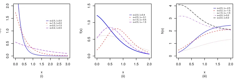
respectively. The limiting distribution of the HLP distribution given by ( 4) when λ → 0+ is limλ →0+F(x) =
1−e−αx
1+e−αx
. Figure 1 shows the plots of the pdf and hrf of the half logistic Poisson distribution.
0.0 0.5 1.0 1.5 2.0 2.5 3.0
0.0 0.5 1.0 1.5 2.0 x f(x) (i)
α=2.5, λ=3.0 α=1.5, λ=2.0 α=3.0, λ=1.5 α=0.2, λ=5.5
0.0 0.5 1.0 1.5 2.0
0.0 0.5 1.0 1.5 x f(x) (ii)
α=2.0, λ=0.4 α=2.5, λ=−3.1 α=1.5, λ=−0.5 α=2.5, λ=−1.5
0.0 0.5 1.0 1.5 2.0
0 1 2 3 4 x h(x) (iii)
α=2.5, λ=−2.5 α=2.2, λ=−1.5 α=1.5, λ=−1.5 α=2.0, λ=3.0 α=2.0, λ=4.0
Figure 1. Plots of the (i), (ii) pdf and (iii) hrf of the HLP distribution for
some selected values of parameters.
The quantile function of the HLP distribution can be used to generate a random data dis-tributed according to HLP(α, λ) whenp∼U(0,1), whereU(0,1) is the uniform distribution. The quantile of X can be presented as
(7) %α,λ(p) =
−1
α log
1−log(1−p−(1λ−e−λ))
1 +log(1−p−(1λ−e−λ))
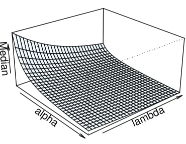
The median of the HLP distribution can be obtained when p = 0.5 in (7). Figure 2 shows that the median is decreasing function in both α and λ >0.
alpha
lambda Median
Figure 2. Plots of the median of the HLP distribution for λ >0
2.1. Moments. The features and characteristics of a distribution can be studied through its moments such as the mean, variance and moment generating function, etc. If X has the HLP (α, λ) distribution, then the rth moment of X (µ
r = E[Xr]) can be computed from
E[Xr] =R∞ 0 x
rf(x)dx as follows
(8) E[Xr] =
Z ∞
0
2αλxre−αx
(1−e−λ)(1 +e−αx)2e
−λ
1−e−αx
1+e−αx
dx,
by letting u = 1−e−αx, then exponential expansion, generalized binomial expansion and
some algebraic manipulations we get
(9) E[Xr] = 2λ
αr(1−e−λ)
∞
X
i=1
∞
X
w=0
(−1)i+rλi i!
−(2 +i)
w
!
∂r
∂crB(i+ 1, w+ 1),
where B(., .) is the complete beta function defined by B(a, b) =R01ua−1(1−u)b−1du and
c=w+ 1. Therefore, the mean (µ1) can be obtain when r= 1 in (9) and variance (σ2) can
be computed from σ2 = E(X2)−(E(X))2
alpha
lambda Mean
alpha
lambda V
ar iance
Figure 3. Plots of the mean and variance of the HLP distribution for λ >0
The moment generating function of the HLP distribution is obtained directly usingMX(t) =
E(etX) which can be expanded to
MX(t) =
∞
X
r=0
tr r!E(X
r),
(10)
hence, by putting ( 9) in ( 10) we have
(11) MX(t) =
2λ αr(1−e−λ)
∞
X
r=0
∞
X
i=1
∞
X
w=0
(−1)i+rtrλi
i!r!
−(2 +i)
w
!
∂r
∂crB(i+ 1, w+ 1).
2.2. Order statistics. LetX1, X2, X3,· · · , Xn be a random sample from HLP distribution,
letX1:n≤X2:n≤ · · · ≤Xn:n,be the order statistics obtained from this random sample, then
for j = 1,2,3,· · · , n, the corresponding pdf, sayfj:n(x) is obtained from
fxj:n(x;α, λ) =
n!
(j −1)!(n−j)!f(x)(F(x))
j−1(1−F(x))n−j,
where f(x) and F(x) are the pdf and cdf of the HLP distribution, we have
fxj:n(x;α, λ) = n−j
X
l=0
n! (−1)l
(j−1)!(n−j−l)!l!f(x)(F(x))
j+l−1
,
using the binomial expansion of Fj+l−1 and after some algebraic manipulations we have
fxj:n(x;α, λ) = n−j
X
l=0
j+l−1 X
k=0
ζj,k,l,n(λ)f(x;α, λ(k+ 1)),
where
ζj,k,l,n(λ) = j+kl−1
n!(−1)
k+l(1−e−λ(k+1))
(1−e−λ)(k+ 1)(j −1)!(n−j −l)!l!,
(13)
and f(x;α, λ(k+ 1)) is the probability density function of the half logistic Poisson distri-bution with parameterα and λ(k+ 1).
The rth-moment of jth order statistic of the HLP distribution is computed using ( 12) as
E(Xr) =
Z ∞
0
xrfxj:n(x;α, λ)dx
(14)
=
n−j
X
l=0
j+l−1 X
k=0
ζj,k,l,n(λ)
Z ∞
0
xrf(x;α, λ(k+ 1))dx (15)
by considering ( 9) we have,
E(Xr) =
n−j
X
l=0
j+l−1 X k=0 ∞ X l=1 ∞ X w=0
ζj,k,l,n,r,w∗ (α, λ) ∂
r
∂crB(i+ 1, w+ 1),
(16)
where ζj,k,l,n,r,w∗ (α, λ) = j+kl−1 −(2+w i)αr2((1−−1)e−i+λk)(+jl−+1)!(rn!λni−(kj+1)−l)!il!i!.
2.3. Shannon entropy. An entropy of a randomvariableX is a measure of variation of the uncertainty. The Shannon entropy of a random variable X with density function given by ( 3) can be defined as E[−logf(x)], we first consider the following lemma and proposition
which are very essential for the computation of the Shannon entropy of the HLP distribution.
Lemma 2.2. For a1 >0 and a2 >0, let
(17) ψ(a1, a2) =
Z ∞
0
(1−e−αx)a1e−αx
(1 +e−αx)a2 e −λ
1−e−αx
1+e−αx
dx,
then,
(18) ψ(a1, a2) =
2λ (1−e−λ)
∞ X i=1 ∞ X w=0
(−1)iλi i!
−(a2+i)
w
!
B(a1+i, w+ 1),
where B(., .) is a complete beta function.
proof. Follow similar in computing (9).
Proposition 2.3. For a random variable X with pdf given by (3), then,
E log (1 +e−αX)= 2αλ (1−e−λ)
∂
∂tψ(0,2−t)|t=0, (19)
E
1−e−αX
1 +e−αX
= 2αλ
(1−e−λ)ψ(1,3).
proof. By using the lemma 2.2.
Thus, we can compute the Shannon entropy of the HLP distribution using (19) and (20) as
E[−logf(X)] = log
1−e−λ
2α λ
+αE(X) + 4αλ (1−e−λ)
∂
∂tφ(0,2−t)|t=0
+ 2αλ
2
(1−e−λ)φ(1,3),
(21)
where E(X) can be calculated using (9) whenr = 1.
3. Estimation
The maximum likelihood ofα and λ can be obtain simultaneously by the numerical solu-tions of ( 23) and ( 24) when set equal to zero using mathematical software such as R and
Mathematica. The total log likelihood function of the half-logistic Poisson distribution is given by
logl(θ) =nlog 2 +nlogα+nlogλ−α
n
X
i=1
xi−λ n
X
i=1
1−e−αxi
1 +e−αxi
−nlog(1−e−λ)−2
n
X
i=1
log(1−e−αxi).
(22)
whereθ = (α, λ)T, the first partial derivative of log`(θ) that is∂log`(θ)/∂αand∂log`(θ)/∂λ are computed as
∂(logl(θ)) ∂α = n α − n X i=1
xi−2λ n
X
i=1
xie−αx
(1 +e−αxi)2 −2
n
X
i=1
xie−αxi
1 +e−αxi,
(23) ∂(logl(θ)) ∂λ = n λ − n X i=1
1−e−αxi
1 +e−αxi
+ ne
−λ
(1−e−λ).
(24)
For a very large sample we apply the usual approximation that the MLEs of the HLP can be approximated as bivariate normal with mean zero and variance covariance matrixI−1(θ),
where I(θ) is the expected information matrix. Alternatively we can use J(θ) the 2 ×2
information matrix defined by J(θ) = −∂2(log∂θ∂θ`T(θ))
. The approximate of the MLEs of θ,
the ˆθ, can be approximated as N2(0, J(ˆθ)−1) under the regularity conditions stated in [13].
The asymptotic distribution of√n(ˆθ−θ) isN2(0, J(ˆθ)−1), whereJ(ˆθ) is the unit information
matrix evaluated at ˆθ, which can be used to construct the approximate confidence interval for each parameter. A 100(1−)% asymptotic confidence interval for each parameter θr is
given by ACIr = (ˆθr−Z2
p
ˆ Irr,θˆ
r+Z2
p
ˆ
In(θ)−1 for r= 1,2 andZ2 is the quantile (1−2) of the standard normal distribution. The
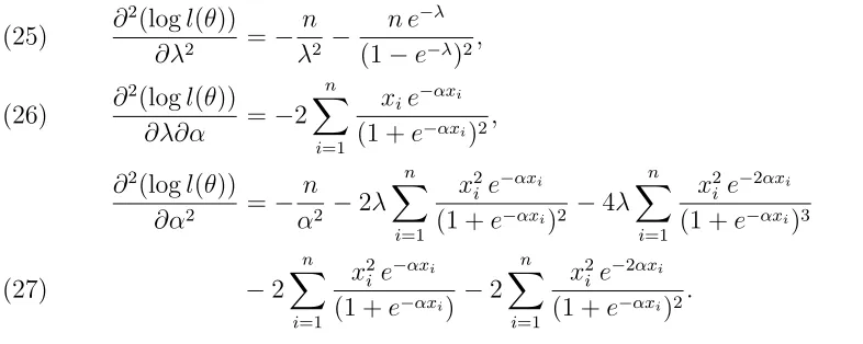
elements of J(θ) are given below
∂2(logl(θ)) ∂λ2 =−
n λ2 −
n e−λ (1−e−λ)2,
(25)
∂2(logl(θ)) ∂λ∂α =−2
n
X
i=1
xie−αxi
(1 +e−αxi)2,
(26)
∂2(logl(θ))
∂α2 =−
n α2 −2λ
n
X
i=1
x2
i e
−αxi
(1 +e−αxi)2 −4λ
n
X
i=1
x2
i e
−2αxi
(1 +e−αxi)3
−2
n
X
i=1
x2
i e
−αxi
(1 +e−αxi) −2
n
X
i=1
x2
i e
−2αxi
(1 +e−αxi)2.
(27)
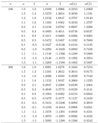
3.1. Simulation study. In this part, we evaluate the performance of the maximum like-lihood estimates using simulation study; we generate 10,000 samples from the HLP (α, λ) distribution, each of sample sizes n=50, 100 and 200, for some selected values of α >0 and λ∈R− {0}. The result of the simulations are displayed in Table 2 below. The result shows that the method of maximum likelihood performed consistently and the standard deviations of the maximum likelihood estimates decrease as we increase the sample size.
Table 1. MLEs and Standard deviations for some values of parameters.
Sample size Actual values Estimated values Standard deviations
n α λ αˆ ˆλ sd( ˆα) sd(ˆλ)
50 1.0 1.0 1.0303 1.0817 0.2771 1.1304
1.5 1.3 1.5794 1.3164 0.4627 1.2191
1.2 1.0 1.2285 1.1003 0.3332 1.1579
1.1 1.8 1.2243 1.7129 0.4027 1.3270
0.2 2.1 0.2385 1.8289 0.1023 1.3820
0.5 0.3 0.4859 0.5607 0.0991 0.8544
0.1 0.8 0.1017 0.9216 0.0257 1.0653
0.5 0.5 0.5515 0.6305 0.1568 0.9587
0.1 -0.5 0.1054 -0.7347 0.0175 0.7079 0.5 -1.0 0.4436 -0.7204 0.113 0.9159
1.1 -1.1 1.1338 -1.2317 0.1847 0.8120 1.2 -1.3 1.2346 -1.4407 0.1949 0.8379
Table 2. MLEs and Standard deviations for some values of parameters.
Sample size Actual values Estimated values Standard deviations
n α λ αˆ ˆλ sd( ˆα) sd(ˆλ)
100 1.0 1.0 1.0109 1.0906 0.2253 1.0369
1.5 1.3 1.5379 1.3654 0.3850 1.1191
1.2 1.0 1.2156 1.0847 0.2707 1.0140
1.1 1.8 1.1482 1.8562 0.3343 1.2707
0.2 2.1 0.2156 2.0782 0.0687 1.3306
0.5 0.3 0.4893 0.4611 0.0748 0.6537
0.1 0.8 0.1011 0.8669 0.0206 0.9265
0.5 0.5 0.5472 0.5487 0.1332 0.7600
0.1 -0.5 0.1027 -0.6136 0.0124 0.5135 0.5 -1.0 0.4293 -0.5828 0.0982 0.7428
1.1 -1.1 1.1148 -1.1566 0.1288 0.5869 1.2 -1.3 1.2146 -1.3570 0.1392 0.5954
1.5 -1.1 1.5202 -1.1580 0.1802 0.5897
200 1.0 1.0 1.0091 1.0278 0.1683 0.7218
1.5 1.3 1.5165 1.3612 0.3014 0.9175
1.2 1.0 1.2096 1.0350 0.2029 0.7548
1.1 1.8 1.1152 1.9107 0.2668 1.1235
0.2 2.1 0.2047 2.2208 0.0539 1.2364
0.5 0.3 0.4949 0.3773 0.0528 0.4141
0.1 0.8 0.1004 0.8382 0.0154 0.6604
0.5 0.5 0.5479 0.4577 0.1127 0.5434
0.1 -0.5 0.1012 -0.5506 0.0092 0.3919
0.5 -0.1 0.4193 -0.4844 0.0908 0.6261 1.1 -1.1 1.1078 -1.1301 0.0948 0.4241
1.2 -1.3 1.2070 -1.3291 0.0986 0.4232 1.5 -1.1 1.5093 -1.1280 0.1286 0.4242
4. Real data illustration
In this section, we provide application of the HLP distribution to a real data for illustration. We consider the AIC (Akaike information criterion), BIC (Bayesian information criteria) and KS (Kolmogorov Smirnov) test statistic for comparison between the HLP distribution and some other existing distributions such as the Olapade generalize half logistic (OGHL) distribution by [39] with cdf given asF(x) = 1− 2θ(1 +ex/α)−θ
, Power half logistic (PwHL) by [23] with cdf F(x) = 1−(2/(1 + exp(θxα))), generalized half logistic (GHL) with cdf
F(x) = (1−exp(−αx))θ(1 + exp(−αx))−θ, GHL distribution appears in the study of its
properties such as the rth-moments, probability weighted moments, Shannon and Renyi entropies can be obtained from [11]. The generalized exponential (GE) with cdf F(x) = (1−exp(−αx))θ by [35], BurrXII (BXII) by [7] withF(x) = 1−(1+xα)−θ, Chen distribution
(Chen) by [9] with F(x) = 1−exp(θ(1− exp(xα))), exponential (E) with F(x) = 1−
exp(−αx), and half logistic (HL)distribution given by ( 2). The model with the smallest value of AIC, BIC and KS provide best fit than the other models.
The data set is provided by [41] and recently analyzed by [20] is the number of successive failures obtained from the air conditioning system of each member in a fleet of 13 Boeing 720 jet airplanes, the data set are: 194, 413, 90, 74, 55, 23, 97, 50, 359, 50, 130, 487, 57, 102, 15, 14, 10, 57, 320, 261, 51, 44, 9, 254, 493, 33, 18, 209, 41, 58, 60, 48, 56, 87, 11, 102, 12, 5, 14, 14, 29, 37, 186, 29, 104, 7, 4 ,72, 270, 283, 7 ,61, 100, 61, 502, 220, 120, 141, 22, 603, 35, 98 ,54, 100, 11, 181, 65 ,49 ,12 ,239, 14 ,18 ,39, 3 ,12, 5 ,32, 9, 438, 43, 134, 184, 20, 386, 182, 71, 80, 188, 230, 152, 5 ,36, 79, 59, 33, 246, 1 ,79, 3 ,27, 201, 84 ,27 ,156, 21 ,16, 88, 130, 14, 118, 44 ,15 ,42, 106 ,46 ,230 ,26, 59 ,153, 104, 20, 206, 5 ,66 ,34, 29, 26, 35 ,5 ,82, 31, 118 ,326 ,12, 54, 36 ,34, 18, 25, 120, 31 ,22 ,18, 216, 139, 67, 310, 3 ,46 ,210, 57, 76 ,14 ,111, 97, 62, 39, 30, 7 ,44, 11, 63, 23 ,22 ,23, 14, 18, 13, 34, 16, 18, 130, 90, 163 ,208, 1 ,24, 70, 16, 101, 52, 208, 95, 62, 11, 191 ,14 ,71.
The computed values of the MLEs, AIC, BIC and KS with its P-value of each model for the given datasets are listed in Table 3, as you can see, the results shows that HLP distribution represent the data better than the other competing distributions. Figur 4 shows the plots of the (i) histogram with fitted HLP and (ii) empirical cdf with the fitted HLP distribution cdf, Figur 5 display the quantile-quantile plot (iii) and hazard rate function of HLP distribution (iv) for the given data set.
Table 3. MLEs, `(Θ), AIC, BIC, KS and p-value for the given data set
Model α λ θ `(Θ) AIC BIC K-S p-value
HLP 0.0069 3.3077 - -1036.261 2076.522 2082.995 0.0572 0.5708
OGHL 1.1419 - 0.0125 -1037.644 2079.288 2085.761 0.0862 0.1227
GHL 0.0120 - 0.7248 -1044.156 2092.312 2098.785 0.1017 0.0409
PwHL 0.7680 - 0.0475 - 1039.484 2082.968 2089.441 0.0628 0.4483
GE 0.0102 - 0.9100 - 1037.750 2079.500 2085.973 0.0728 0.2718
BXII 1.0801 - 0.2317 - 1180.456 2364.912 2371.385 0.3681 0.0000
Chen 0.2582 - 0.0396 -1053.409 2110.818 2117.291 0.1013 0.0422
HL 0.0145 - - -1051.020 2104.040 2107.270 0.1538 2.9e-4
x
Density
0 100 300 500
0.000
0.004
0.008
(i) HLP Empirical
0 100 200 300 400 500 600
0.0
0.4
0.8
x
cdf
HLP Empirical
(ii)
Figure 4. Plots of (i) histogram with fitted HLP and (ii) empirical cdf with
fitted HLP cdf.
0 100 200 300 400 500 600
0
200
500
HLP−quantiles
Sample quantiles
(iii)
0 200 400 600 800
0.007
0.010
x
h(x)
(iv)
Figure 5. (iii) Quantile-quantile plot and (iv) hazard rate function of HLP.
5. Conclusions
We proposed and study a new two-parameter lifetime distribution called the half-logistic Poisson (HLP) distribution. We provide several properties of the new distribution in which we derive an explicit formula for the rth moment, moment generating function, order
parameters of the distribution by the method of maximum likelihood and assessed by sim-ulation studies. The usefulness of the HLP distribution is illustrated by means of real data set in which HLP provide better fit than some other popular models.
Acknowledgement
The author would like to thank the referees for their useful suggestions.
References
[1] Alaa H Abdel-Hamid. Properties, estimations and predictions for a poisson-half-logistic distribution based on progressively type-ii censored samples.Applied Mathematical Mod-elling, 40(15):7164–7181, 2016.
[2] K Adamidis and S Loukas. A lifetime distribution with decreasing failure rate.
Statistics & Probability Letters, 39(1):35–42, 1998.
[3] Bander Al-Zahrani and Hanaa Sagor. The poisson-lomax distribution. Revista Colom-biana de Estad´ıstica, 37(1):225–245, 2014.
[4] Sumeet H Arora, GC Bihmani, and MN Patel. Some results on maximum likelihood estimators of parameters of generalized half logistic distribution under type-i progressive censoring with changing failure rate. International Journal Of Contemporary Mathe-matical Sciences, 5(14):685–698, 2010.
[5] Hassan S Bakouch, Mansour Aghababaei Jazi, Saralees Nadarajah, Ali Dolati, and Rasool Roozegar. A lifetime model with increasing failure rate. Applied Mathematical Modelling, 38(23):5392–5406, 2014.
[6] Hassan S Bakouch, Miroslav M Risti´c, A Asgharzadeh, L Esmaily, and Bander M Al-Zahrani. An exponentiated exponential binomial distribution with application.Statistics & Probability Letters, 82(6):1067–1081, 2012.
[7] Irving W Burr. Cumulative frequency functions. The Annals of Mathematical Statistics, 13(2):215–232, 1942.
[8] Vicente G Cancho, Franscisco Louzada-Neto, and Gladys DC Barriga. The poisson-exponential lifetime distribution. Computational Statistics & Data Analysis, 55(1):677– 686, 2011.
[9] Zhenmin Chen. A new two-parameter lifetime distribution with bathtub shape or in-creasing failure rate function. Statistics & Probability Letters, 49(2):155–161, 2000. [10] Gauss M Cordeiro, Morad Alizadeh, and Pedro Rafael Diniz Marinho. The type i
[11] Gauss M Cordeiro, Morad Alizadeh, and Edwin MM Ortega. The exponentiated half-logistic family of distributions: Properties and applications. Journal of Probability and Statistics, 2014, 2014.
[12] Gauss Moutinho Cordeiro and Rodrigo Bernardo da Silva. A classe complementar de distribui¸c˜oes weibull estendida s´eries de potˆencia. Ciencia & Natura, 36(3):1–13, 2014. [13] D.R Cox and D.V Hinkely. Theoretical statistics. Chapman & Hall, London, 1979. [14] Ronaldo V da Silva, Frank Gomes-Silva, Manoel Wallace A Ramos, and Gauss M
Cordeiro. The exponentiated burr xii poisson distribution with application to lifetime data. International Journal of Statistics and Probability, 4(4):112, 2015.
[15] Ibrahim Elbatal, M. M Mansour, and Mohammad Ahsanullah. The additive weibull-geometric distribution: Theory and applications. Journal of Statistical Theory and Applications, 15(2):125–141, 2016.
[16] Wenhao Gui, Shangli Zhang, and Xinman Lu. The lindley-poisson distribution in lifetime analysis and its properties. Hacttepe Journal of Mathematics and Statistics, 43(6):1063–1077, 2014.
[17] Amal Hassan, Salwa Assar, and Kareem Ali. The complementary poisson-lindley class of distributions. International Journal of Advanced Statistics and Probability, 3(2):146– 160, 2015.
[18] Amal S. Hassan, Abd-Elfattah A.M, and Asmaa H. Mokhtar. The complementary burr iii poisson distribution. Australian Journal of Basic and Applied Sciences, 9(11):219– 228, 2015.
[19] Amal S. Hassan, Abd Elfattah AM, and Asmaa H Mokhtar. The complementary ex-ponentiated inverted weibull power series family of distributions and its applications.
British Journal of Mathematics Computer Science, 13(2):1–20, 2016.
[20] Shujiao Huang and Broderick O Oluyede. Exponentiated kumaraswamy-dagum distri-bution with applications to income and lifetime data. Journal of Statistical Distributions and Applications, 1, 2014.
[21] Suk-Bok Kang and Jung-In Seo. Estimation in an exponentiated half logistic distribution under progressively type-ii censoring. Communications for Statistical Applications and Methods, 18(5):657–666, 2011.
[22] RRL Kantam, V Ramakrishna, and MS Ravikumar. Estimation and testing in type i generalized half logistic distribution. Journal of Modern Applied Statistical Methods, 12(1):22, 2013.
[23] SREEKRISHNANILAYAM DEVAKIAMMA Krishnarani. On a power transformation of half-logistic distribution. Journal of Probability and Statistics, 2016, 2016.
[25] Francisco Louzada, Vitor Marchi, and James Carpenter. The complementary exponen-tiated exponential geometric lifetime distribution. Journal of Probability and Statistics, 2013, 2013.
[26] Francisco Louzada, Mari Roman, and Vicente G Cancho. The complementary exponen-tial geometric distribution: Model, properties, and a comparison with its counterpart.
Computational Statistics & Data Analysis, 55(8):2516–2524, 2011.
[27] E. Mahmoudi, A. Sepahdar, and A. Lemonte. Exponentiated Weibull-logarithmic Dis-tribution: Model, Properties and Applications. ArXiv e-prints, February 2014.
[28] Eisa Mahmoudi and Ali Akbar Jafari. Generalized exponential–power series distribu-tions. Computational Statistics & Data Analysis, 56(12):4047–4066, 2012.
[29] Eisa Mahmoudi and Ali Akbar Jafari. The compound class of linear failure rate-power se-ries distributions: Model, properties and applications. arXiv preprint arXiv:1402.5282, 2014.
[30] Eisa Mahmoudi and Afsaneh Sepahdar. Exponentiated weibull–poisson distribution: Model, properties and applications. Mathematics and Computers in Simulation, 92:76– 97, 2013.
[31] Eisa Mahmoudi and Mitra Shiran. Exponentiated weibull-geometric distribution and its applications. arXiv preprint arXiv:1206.4008, 2012.
[32] Eisa Mahmoudi and Mitra Shiran. Exponentiated weibull power series distributions and its applications. arXiv preprint arXiv:1212.5613, 2012.
[33] Ghorbani Mehrzad, Fazel Bagheri Seyed, and Alizadeh Mojtaba. A new family of distributions: The additive modified weibull odd log-logistic-g poisson family, properties and applications. Annals of Data Science, pages 1–39, 2017.
[34] Alice Lemos Morais and Wagner Barreto-Souza. A compound class of weibull and power series distributions. Computational Statistics & Data Analysis, 55(3):1410–1425, 2011. [35] Govind S Mudholkar and Deo Kumar Srivastava. Exponentiated weibull family for
analyzing bathtub failure-rate data. IEEE Transactions on Reliability, 42(2):299–302, 1993.
[36] Mustapha Muhammad. A Mixed BurrXII and Zero truncated Poisson distribution: model, properties and application. Faculty of Graduate Studies, Jordan University of Science and Technology, Jordan (Unpublished), Msc. Thesis, 2012.
[39] A. K. Olapade. The type i generalized half logistic distribution. Journal of the Iranian Statistical Society, 13(1):69–82, 2014.
[40] Broderick O Oluyede, Galelhakanelwe Motsewabagale, Shujiao Huang, Gayan Warahena-Liyanage, and Mavis Pararai. The dagum-poisson distribution: model, prop-erties and application. Electronic Journal of Applied Statistical Analysis, 9(1):169–197, 2016.
[41] F Proschan. Theoretical explanation of observed decreasing failure rate. Technometrics, pages 375–383, 1963.
[42] Miroslav M Risti´c and Saralees Nadarajah. A new lifetime distribution. Journal of Statistical Computation and Simulation, 84(1):135–150, 2014.
[43] Jung-In Seo, Yongku Kim, and Suk-Bok Kang. Estimation on the generalized half logistic distribution under type-ii hybrid censoring. Communications for Statistical Ap-plications and Methods, 20(1):63–75, 2013.
[44] Jung-In Seo, Hwa-Jung Lee, and Suk-Bok Kan. Estimation for generalized half logistic distribution based on records. Journal of the Korean Data and Information Science Society, 23(6):1249–1257, 2012.
[45] Rodrigo B Silva, Marcelo Bourguignon, C´ıcero RB Dias, and Gauss M Cordeiro. The compound class of extended weibull power series distributions. Computational Statistics & Data Analysis, 58:352–367, 2013.
[46] Rodrigo B Silva and Gauss M Cordeiro. The burr xii power series distributions: A new compounding family. Submitted to the Brazilian Journal of Probability and Statistics, 2013.
[47] Saeid Tahmasebi and Ali Akbar Jafari. Generalized gompertz-power series distributions.
arXiv preprint arXiv:1508.07634, 2015.
[48] Cynthia Tojeiro, Francisco Louzada, Mari Roman, and Patrick Borges. The complemen-tary weibull geometric distribution. Journal of Statistical Computation and Simulation, 84(6):1345–1362, 2014.
[49] Min Wang and Ibrahim Elbatal. The modified weibull geometric distribution. Metron, 73(3):303–315, 2015.
Department of Mathematical Science, Bayero University Kano, Nigeria,