The Thirty-Third AAAI Conference on Artificial Intelligence (AAAI-19)
TAPAS: Train-Less Accuracy Predictor for Architecture Search
R. Istrate,
1,2F. Scheidegger,
1G. Mariani,
1D. Nikolopoulos,
2C. Bekas,
1A. C. I. Malossi
11IBM Research – Zurich, Switzerland 2University of Belfast, United Kingdom
Abstract
In recent years an increasing number of researchers and practitioners have been suggesting algorithms for large-scale neural network architecture search: genetic algorithms, rein-forcement learning, learning curve extrapolation, and accu-racy predictors. None of them, however, demonstrated high-performance without training new experiments in the pres-ence of unseen datasets. We propose a new deep neural network accuracy predictor, that estimates in fractions of a second classification performance for unseen input datasets, without training. In contrast to previously proposed ap-proaches, our prediction is not only calibrated on the topo-logical network information, but also on the characterization of the dataset-difficulty which allows us to re-tune the pre-diction without any training. Our predictor achieves a perfor-mance which exceeds 100 networks per second on a single GPU, thus creating the opportunity to perform large-scale ar-chitecture search within a few minutes. We present results of two searches performed in 400 seconds on a single GPU. Our best discovered networks reach 93.67% accuracy for CIFAR-10 and 81.01% for CIFAR-CIFAR-100, verified by training. These networks are performance competitive with other automati-cally discovered state-of-the-art networks however we only needed a small fraction of the time to solution and computa-tional resources.
1
Introduction
Automatic generation and tuning of convolutional neural network (CNN) architectures is a growing research topic. The majority of approaches in the literature (for a deep overview, see Section 2) are rooted into the fundamen-tal idea of large-scale explorations; more precisely, they can be based either on evolution and mutations (Real et al. 2017; Xie and Yuille 2017; Miikkulainen et al. 2017), or on reinforcement learning (Zhong, Yan, and Liu 2017; Zoph and Le 2016; Zoph et al. 2017; Cai et al. 2018; Baker et al. 2016). All these algorithms require a large amount of training experiments which quickly leads to mas-sive resource and time to solution requirements.
Recently, the concept of performance prediction for ar-chitecture search has emerged. The fundamental idea is to drastically reduce exploration cost, by forecasting accuracy
Copyright c2019, Association for the Advancement of Artificial Intelligence (www.aaai.org). All rights reserved.
of networks without (or with very limited) training. Predic-tion is obtained either from partial learning curves (Domhan, Springenberg, and Hutter 2015; Klein et al. 2017; Baker et al. 2018; Swersky, Snoek, and Adams 2014), or from a database of trained experiments (Deng, Yan, and Lin 2017). The former approach requires partial training of each spe-cific network. The latter one, implies training hundreds of networks on the given input dataset, to build a reliable ground-truth. Thus, none of them can be used out-of-the-box for near real-time architecture search.
In this work, we introduce a train-less accuracy predic-tor for architecture search (TAPAS), that provides reliable architecture peak accuracy predictions when used with un-seen (i.e., not previously un-seen by the predictor) datasets. Our accuracy predictor is train-less in the sense that it estimates the accuracy of a network on a dataset without training the network. This is achieved by adapting the prediction to the difficultyof the dataset, that is automatically determined by the framework. In addition, we reuse experience accumu-lated from previous experiments. The main features of our framework are summarized as follows: (i) it is not bounded to any specific dataset, (ii) it learns from previous experi-ments, whatever dataset they involve, improving prediction over usage and (iii) it allows to run large-scale architecture search on a single GPU device within a few minutes.
In summary, our main contributions are the following: i) a fast, scalable, and reliable framework for CNN architecture performance prediction; ii) a flexible prediction algorithm, that dynamically adapts to the difficulty of the input; iii) an extensive comparison with preexisting methods/results, clearly illustrating the advantages of our approach.
In Section 2 we briefly review literature approaches and analyze pros and cons of each of them. In Section 3 we present the design of our prediction framework, with a deep dive into its three main components. Then, in Section 4 we compare experimental results with current state-of-the-art. An additional discussion and final conclusions are summa-rized in Sections 5 and 6, respectively.
2
Related work
DC DCN LDE
≈ mins
TAP
TAP DCN
Accuracy
Training phase
Prediction phase
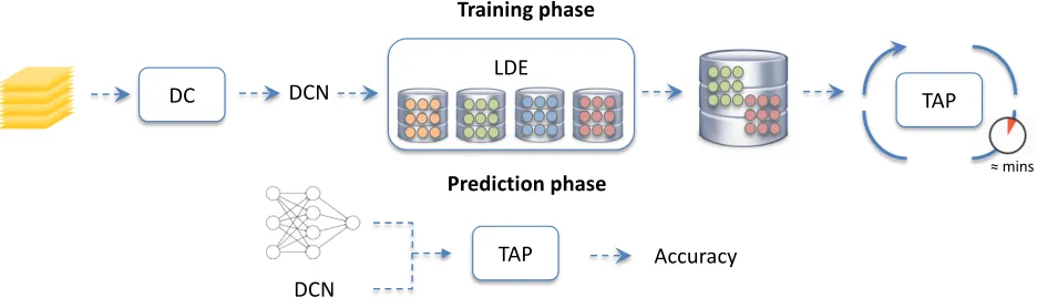
Figure 1: Schematic TAPAS workflow. First row: the Dataset Characterization (DC) takes a new, unseen dataset and charac-terizes its difficulty by computing the Dataset Characterization Number (DCN). This number is then used to select a subset of experiments executed on similarly difficult datasets from the Lifelong Database of Experiments (LDE). Subsequently, the filtered experiments are used to train the Train-less Accuracy Predictor (TAP), an operation that takes up to a few minutes. Sec-ond row: the trained TAP takes the network architecture structure and the dataset DCN and predict the peak accuracy reachable after training. This phase scales very efficiently in a few seconds over a large number of networks.
receives a layer-by-layer encoding. In contrast to our ap-proach, they encode an epoch number and predict the ac-curacy at the given epoch. Peephole delivers good perfor-mance on MNIST and CIFAR-10, however it has not been designed to transfer knowledge from familiar datasets to unseen ones. Given a new dataset, hundreds of networks need to be trained before Peephole makes a prediction. In contrast, our framework is designed to operate on unseen datasets, without the need of expensive training.
Accuracy predictors such as learning curves extrapo-lation (LCE) (Domhan, Springenberg, and Hutter 2015), BNN (Klein et al. 2017), ν-SVR (Baker et al. 2018) fore-cast network performance based on partial learning curves. These algorithms are designed in the context of hyperpa-rameter optimization or meta-learning. Both cases require extensive use of training and thus result in high compu-tational costs. Moreover, they are all dataset and network specific, i.e., the prediction cannot be transferred to another network or dataset, without re-training. In particular, LCE employs a weighted probabilistic model to predict network performance. BNN uses Bayesian Neural Networks to fit completely new learning curves and extrapolate partially observed ones. This approach yields superior performance compared to LCE, particularly at stages where the initial observed learning curve is not sufficient for the paramet-ric algorithm to converge. Nevertheless, both methods rely on expensive Markov Chain Monte Carlo sampling proce-dures. ν-SVR (Baker et al. 2018) complements the infor-mation on the learning curve with network architecture de-tails and a list of predefined hyperparameters. These are used to train a sequence of regression models, that outper-form LCE and BNN. Although these methods exhibit good performance, they require a considerable part of the initial learning curve to provide reliable performance.
Large-scale exploration algorithms (Real et al. 2017; Xie and Yuille 2017; Miikkulainen et al. 2017; Zhong,
Yan, and Liu 2017; Zoph and Le 2016; Zoph et al. 2017; Cai et al. 2018; Baker et al. 2016; Pham et al. 2018) em-ploy genetic mutations or reinforcement learning to explore a large space of architecture configurations. Regardless of the approach, all these methods train a large number of net-works, some of them employing hundreds of GPUs for more than ten days (Real et al. 2017). ENAS (Pham et al. 2018) uses a controller to discover CNN architectures, by search-ing for an optimal subgraph within a large computational graph. With this approach it discovers a 97.11% accurate network for CIFAR-10, on a single GPU in 10 hours. While ENAS reduces drastically the time-to-solution compared to previous results, the model is applied to only one dataset and not generalized to the case of multiple datasets. Indeed, shar-ing parameters among child models for different datasets is not straightforward.
3
Methodology
In this section, we provide a detailed overview of the main building blocks of the TAPAS framework. TAPAS aims to reliably estimate peak accuracy at low cost for a variety of CNN architectures. This is achieved by leveraging a com-pact characterization of the user-provided input dataset, as well as a dynamically growing database of trained neural networks and associated performance. The TAPAS frame-work, depicted in Figure 1, is built on three main compo-nents:
1. Dataset Characterization (DC): Receives an unseen dataset and computes a scalar score, namely the Dataset Characterization Number (DCN) (Scheidegger et al. 2018), which is used to rank datasets;
2. Lifelong Database of Experiments (LDE): Ingests training experiments of NNs on a variety of image classi-fication datasets executed inside the TAPAS framework;
ar-MNIST
GTSRB
(Crop) SVHN
GTSRB
F
ashion
MNIST
Imagenet
S1
CIF
AR-10
Imagenet
S2
Flo
w
ers-5
Imagenet
S3
STL-10
Imagenet
S4
Imagenet
S5
CIF
AR-100
Imagenet
S6
Flo
w
ers-102
Imagenet
S7
Imagenet
S8
F
oo
d
0.0 0.5 1.0
DCN Real datasets
ImageNet subsets
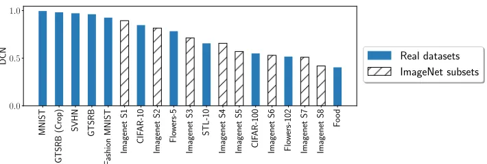
Figure 2: List of image classification datasets used for characterization. The datasets are sorted by the DCN value from the easiest (left) to the hardest (right).
chitecture and a DCN, it predicts the potentially reach-able peak accuracy without training the network.
3.1
Dataset characterization (DC)
The same CNN can yield different results if trained on an easy dataset (e.g., MNIST (Deng 2012)) or on a more challenging one (e.g., CIFAR-100 (Krizhevsky and Hinton 2009)), although the two datasets might share features such as number of classes, number of images, and resolution. Therefore, in order to reliably estimate a CNN performance on a dataset we argue that we must first analyze the dataset difficulty. We compute the DCN by training a probe net to obtain a dataset difficulty estimation (Scheidegger et al. 2018). We use the DCN for filtering datasets from the LDE and directly as input score in the TAP training and prediction phases as described in Section 3.3.
DCN computation Prob netsare modest-sized neural net-works designed to characterize the difficulty of an image classification dataset (Scheidegger et al. 2018). We com-pute the DCN as peak accuracy, ranged in[0,1], obtained by training theDeep normalized ProbeNeton a specific dataset for ten epochs. The DCN calculation cost is low due the following reasons: (i) Deep norm ProbeNet is a modest-size network, (ii) the characterization step is performed only once at the entry of the dataset in the framework (the LDE stores the DCN afterwards), (iii) the DCN does not require an extremely accurate training, thus reducing the cost to a few epochs, and (iv) large datasets can be subsampled both in terms of number of images and of pixels.
The DCN is a rough estimation of the dataset difficulty, and is thus tolerant to approximations. In Section 4 we pro-vide epro-vidence of the effect of the DCN on the TAP.
3.2
Lifelong database of experiments (LDE)
LDE is a continuously growing DB, which ingests every new experiment effectuated inside the framework. An exper-iment includes the CNN architecture description, the train-ing hyper-parameters, the employed dataset (with its DCN), as well as the achieved accuracy.
LDE initialization At the very beginning, the LDE is empty. Thus we perform a massive initialization procedure to populate it with experiments. For each available dataset in
Figure 2 we sample 800 networks from a slight variation of the space of MetaQNN (Baker et al. 2016). For convolution layers we use strides with values in{1,2}, receptive fields with values in{3,4, ..256}, padding in{same, valid}and whether is batch normalized or not. We also add two more layer types to the search space: residual blocks and skip con-nections. The hyperparameters of the residual blocks are the receptive field, stride and the repeat factor. The receptive field and the stride have the same bounds as in the convo-lution layer, while the repeat factor varies between 1 and 6 inclusively. The skip connection has only one hyperparame-ter, namely the previous layer to be connected to.
To speed up the process, we train the networks one layer at a time using the incremental method described in (Istrate et al. 2017). In this way we obtain the accuracies of all inter-mediary sub-networks at the same cost of the entire one. To facilitate the TAP, we train all networks with the same hyper-parameters, i.e., same optimizer, learning rate, batch size, and weights initiallizer. Although the fixed hyper-parameter setting seems a strong limitation and might limit peak accu-racy by a few percent, it is enough to trim poorly performing networks and, in the case of an architecture search, to fairly rank competitive networks, the performance of which can later be optimized further, as discussed in Section 4. As data augmentation we use standard horizontal flips, when possi-ble, and left/right shifts with four pixels. For all datasets we perform feature-wise standardization.
This paper LDE initialization takes 18 months on a sin-gle P100 GPU. This number can be scaled down embar-rassingly with the number of GPUs. It must also be con-sidered that, even though the time spent to generate the LDE is comparable to the time of manual engineering search of hyperparameters, the LDE can then be employed in archi-tecture searches for multiple datasets at no additional cost. Moreover, in an industrial environments, pre-existing runs on technical propriertary-datasets can be used to heat-up the LDE quickly.
relation
kDCN( ˆD)−DCN(Dj)k ≤τ j∈[1, Nd], (1) whereτis a predefined threshold that, in our experiments, is set to 0.05.
3.3
Train-less accuracy predictor (TAP)
TAP is designed to perform fast and reliable CNN accu-racy predictions. Compared to Peephole (Deng, Yan, and Lin 2017), TAP leverages knowledge accumulated through experiments of datasets of similar difficulty filtered from the LDE based on the DCN. Additionally, TAP does not first analyze the entire NN structure and then makes a predic-tion, but instead performs an iterative prediction as depicted in Figure 3. In other words, it aims to predict the accuracy of a sub-networkl1:i+1, assuming the accuracy of the sub-networkl1:i is known. The main building elements of the predictor are: (i) a compact encoding vector that represents the main network characteristics, (ii) a quickly-trainable net-work of LSTMs, and (iii) a layer-by-layer prediction mech-anism.
Neural network architecture encoding Similar to Peep-hole, TAP employs a layer-by-layer encoding vector as de-scribed in Figure 3. Unlike Peephole, we encode more com-plex information of the network architecture for a better pre-diction.
Let us consider a network withNllayers,libeing thei -th layer counting from -the input, wi-thi = 1, . . . , Nl. We define a CNN sub-network as la:b with 1 ≤ a < b ≤ Nl. Our encoding vector contains two types of information as depicted in Figure 3 a): (i) i-th layer information and (ii)l1:i sub-network information. For the currenti-th layer we make the following selection of parameters:Layer type is a one-hot encoding that identifies either convolution, pool-ing, batch normalization, dropout, residual block, skip con-nection, or fully connected. In future we will include lat-est motifs present in literature such as DenseNets (Huang et al. 2017) or AmoebaNets (Real et al. 2018). Note that for the shortcut connection of the residual block we use both the identity and the projection shortcuts (He et al. 2016). The projection is employed only when the residual block decreases the number of filters as compared to the previous layer. Moreover, as compared to (Deng, Yan, and Lin 2017), our networks do not follow a fixed skeleton in the convolu-tional pipeline, allowing for more generality. We only force a fixed block at the end, by using a global pooling and a fully connected layer to prevent networks from overfitting (Lin, Chen, and Yan 2013).
The ratio between the output height and input height of each layer accounts for different strides or paddings, whereas theratio between the output depth and input depth accounts for modifications of the number of kernels. The number of weightsspecifies the total of learnable parameters inli. This value helps the TAP differentiate between layers that increase the learning power of the network (e.g., con-volution, fully connected layers) and layers that reduce the dimensionality or avoid overfitting (e.g., pooling, dropout). In the second part of the encoding vector, we include: To-tal number of layers, counting from input to li, Inference
FLOPsandInference memorythat are an accurate estimate of the computational cost and memory requirements of the sub-network, and finally Accuracy, which is set either to 1/Nc, for the first layer, whereNc is the number of classes to predict, zero for prediction purposes, or a specific value Ai ∈ [0,1]that is obtained from the previous layer predic-tion. Before training, we perform a feature-wise standardiza-tion of the data, meaning that for each feature of the encod-ing vector, we subtract the mean and divide by the standard deviation.
TAP architecture TAP is a neural network consisting of two stacked LSTMs of 50 and 100 hidden units, respectively, followed by a single-output fully connected layer with sig-moid activation. The TAP network has two inputs. The first input is a concatenation of two encoding vectors correspond-ing to layer li andli+1, respectively. This input is fed into the first LSTM. The second input is the DCN and is con-catenated with the output of the second LSTM and then fed into the fully connected layer.
TAP training TAP requires a significant amount of train-ing data to make reliable predictions. The LDE provides this data as described in Section 3.2. As mentioned above, all our generated networks are trained in an incremental fashion, as presented in (Istrate et al. 2017), meaning that for each net-work of length Nl we train all intermediary sub-networks l1:k with1 < k ≤ Nland save their performanceAk. We encode each set of two consecutive layersliandli+1 follow-ing the schema detailed in 3.3, settfollow-ing the accuracy field in the encoding vector oflitoAi, which was obtained through training, and aiming to predictAi+1.
TAP is trained with RMSprop (Tieleman and Hinton 2012), using a learning rate of10−3, a HeNormal weight ini-tialization (He et al. 2015), and a batch size of 512. As the architecture of the TAP is very small, the training process is of the order of a few minutes on a single GPU device. Moreover, the trained TAP can be stored and reapplied to other datasets with similar DCN numbers without the need for retraining.
TAP prediction TAP employs a layer-by-layer prediction mechanism. The accuracy Ai of the sub-networkl1:i pre-dicted by the previous TAP evaluation is subsequently fed as input into the next TAP evaluation, which returns the pre-dicted accuracy Ai+1of the sub-networkl1:i+1. This mech-anism is described more in detail in Figure 3 b).
4
Experiments
In this section, we demonstrate TAPAS performance over a wide range of experiments. Results are compared with ref-erence works from the literature. All runs involve single-precision arithmetic and are performed on IBM1 POWER8
compute nodes, equipped with four NVIDIA P100 GPUs.
1
a)
b)
Layer type Output/Input height ratio Number of weights Total number of layers Inference FLOPs Inference memory Accuracy
Layer 2 Layer 1
Layer 3
Layer !"
TAP DCN
TAP DCN
TAP DCN
Output/Input depth ratio
#$%
1 !'
0 Concat
Concat
#(
0
Concat 0
#$%)*
Figure 3: Encoding vector structure and its usage in the iterative prediction. a) The encoding vector contains two blocks:i -layer information and from input toi-layer sub-network information. b) The encoding vector is used by the TAP following an iterative scheme. Starting from Layer 1 (input) we encode and concatenate two layers at a time and feed them to the TAP. In the concatenated vector, theAccuracyfield Aiofliis set to the predicted accuracy obtained from the previous TAP evaluation, whereas the one ofAi+1corresponding toli+1is always set to zero. For the input layer, we set A0to1/Nc, whereNcis the number of classes, assuming a random distribution. The final predicted accuracyANlis the accuracy of the complete network.
0.00 0.25 0.50 0.75 1.00
Accuracy after training
0.0 0.2 0.4 0.6 0.8 1.0
Predicted
accuracy
MSE = 0.0046 Tau = 0.589
R2= 0.871 Peephole
0.00 0.25 0.50 0.75 1.00
Accuracy after training
0.0 0.2 0.4 0.6 0.8 1.0
MSE = 0.0016 Tau = 0.736
R2= 0.952 LCE
0.00 0.25 0.50 0.75 1.00
Accuracy after training
0.0 0.2 0.4 0.6 0.8 1.0
MSE = 0.0007 Tau = 0.866
R2= 0.979 TAP without DCN
0.00 0.25 0.50 0.75 1.00
Accuracy after training
0.0 0.2 0.4 0.6 0.8 1.0
MSE = 0.0004 Tau = 0.881
R2= 0.987
Scena
rio
A:
CIF
AR-10
TAP
0.00 0.25 0.50 0.75 1.00
Accuracy after training
0.0 0.2 0.4 0.6 0.8 1.0
Predicted
accuracy
MSE = 0.0175 Tau = 0.780
R2= 0.796
0.00 0.25 0.50 0.75 1.00
Accuracy after training
0.0 0.2 0.4 0.6 0.8 1.0
MSE = 0.0098 Tau = 0.811
R2= 0.894
0.00 0.25 0.50 0.75 1.00
Accuracy after training
0.0 0.2 0.4 0.6 0.8 1.0
MSE = 0.0078 Tau = 0.832
R2= 0.908
0.00 0.25 0.50 0.75 1.00
Accuracy after training
0.0 0.2 0.4 0.6 0.8 1.0
MSE = 0.0016 Tau = 0.894
R2= 0.981
Scena
rio
B:
All
datasets
Figure 4: Superior predictive performance of TAP compared with state-of-the-art methods, both when trained on only one dataset (Scenario A) or on multiple datasets (Scenario B).
4.1
Dataset selection for LDE initialization
All the experiments are based on a LDE populated with nine-teen datasets, ranked by difficulty in Figure 2. Eleven of them are publicly available. The other eight are generated
cross-0.0 0.2 0.4 0.6 0.8 1.0
Accuracy after training
0.0 0.2 0.4 0.6 0.8 1.0
Predicted
accuracy
MSE = 0.0483 Tau = 0.386 R2= 0.280 TAP without DCN and LDE filtering
0.0 0.2 0.4 0.6 0.8 1.0
Accuracy after training
0.0 0.2 0.4 0.6 0.8 1.0
MSE = 0.0068 Tau = 0.811 R2= 0.898 TAP without LDE filtering
0.0 0.2 0.4 0.6 0.8 1.0
Accuracy after training
0.0 0.2 0.4 0.6 0.8 1.0
MSE = 0.0040 Tau = 0.846 R2= 0.941
Scena
rio
C:
Unseen
dataset
TAP
Figure 5: Predicted vs real performance (i.e., after training) for Scenario C. Left plot: TAP trained without DCN or LDE pre-filtering. Middle plot: TAP trained with DCN, but LDE is not pre-filtered. Right plot: TAP trained only on LDE experiments with similar dataset difficulty, according to (1).
Predicted Trained Reference
1st 91.94% 93.67% 94.6%
2nd 91.73% 93.41%
-3rd 91.76% 93.31%
-0 100 200 300 400
Wall time (seconds)
0.0 0.2 0.4 0.6 0.8 1.0
Predicted
accuracy
(%)
CIFAR-10
Predicted Trained Reference
1st 80.45% 81.01% 77%
2nd 80.92% 80.45%
-3rd 80.28% 80.63%
-0 100 200 300 400
Wall time (seconds)
0.0 0.2 0.4 0.6 0.8 1.0
Predicted
accuracy
(%)
CIFAR-100
Figure 6: Simulation of large-scale evolution, with 20k mutations. The table compares top three networks (predicted and trained accuracy) with reference work (Real et al. 2017). The simulations require only2×1011FLOPs per dataset, while training the top-three networks for 100 epochs is an additional3×1015FLOPs, causing a 6 hour runtime on a single GPU. The reference work employs9×1019(CIFAR-10) and2×1020FLOPs (CIFAR-100) causing a runtime of 256 hours on 250 GPUs.
validation experiment presented later. Additional details are provided in the Appendix. We resize all dataset images to 32×32pixels. On the one hand, this reduces the cost of LDE initialization, on the other hand, it allows us to poten-tially test networks and datasets in an All2Allfashion. We remark that this choice does not lead to a loss of general-ity, as images of different sizes can be employed in the same pipeline. For every dataset, we generate 800 networks based on the procedure described in Section 3.2. All networks are trained under the same settings: RMSprop optimizer with a learning rate of10−3, weight decay10−4, batch size 64, and HeNormal weight initialization.
4.2
TAPAS performance evaluation
In this section, we define three different scenarios to com-pare TAPAS with LCE (Domhan, Springenberg, and Hutter 2015), BNN (Klein et al. 2017),ν-SVR (Baker et al. 2018) and Peephole (Deng, Yan, and Lin 2017). We employ three evaluation metrics: (i) themean squared error (MSE), which
measures the difference between the estimator and what is estimated, (ii)Kendall’s Tau (Tau), which measures the sim-ilarities of the ordering between the predictions and the real values, and (iii) thecoefficient of determination(R2), which measures the proportion of the variance in the dependent variable that is predictable from the independent variable. In the first metric, lower is better (zero is best); in the others, higher is better (one is best).
Scenario A: Prediction based on experiments on a single dataset We train the TAP on a filtered list of experiments from the LDE based on the CIFAR-10 dataset. We recognize that this scenario is very favorable for prediction, however it is used in reference publications, and therefore allows for a fair comparison.
TAP outperforms all methods, in terms of all the considered metrics. Moreover, if we modify TAP to not use the DCN, we still get better predictions than with all the other methods. The TAP prediction performance is not strongly affected be-cause the training and prediction involve only one dataset.
We argue that the lower results of the Peephole method, as compared to the original paper, are due to the more com-plicated structure of the network we used in our benchmark. Specifically, the Peephole-encoding tuple (layer type, ker-nel height, kerker-nel width, chanker-nels ratio) is not sufficient to predict complicated structures like ResNets.
Scenario B: Prediction based on experiments on all datasets This scenario is similar to Scenario A, but we do not filter experiments by dataset. The second row of Figure 4 shows results when TAP is trained on all datasets, regard-less of their DCN. Also in this scenario, TAP outperforms all methods in all of the considered metrics. We recognize that Peephole is designed to be dataset-specific. However, compared to TAP without DCN the comparison is fair, as neither of these algorithms contain information about the dataset difficulty.
Scenario C: Prediction based on experiments on unseen datasets This scenario aims (i) to demonstrate TAPAS performance when targeting completely unseen datasets and (ii) to highlight importance of dataset-difficulty character-ization and LDE pre-filtering. To do that, we consider the list of datasets in Figure 2 and perform eleven leave-one-out cross-validation benchmarks, considering only the real datasets. The result of this experiment is presented in Fig-ure 5. From left to right, we observe the cumulative impact of the DCN awareness in the TAP training, as well as of the pre-filtering of the experiments in the LDE according to (1). Moreover, by comparing the rightmost plot and metrics with previous results in Figure 4, we observe that TAPAS perfor-mance does not diminish significantly when applied to an unknown dataset.
4.3
Simulated large-scale evolution of image
classifiers
The TAP can be plugged into any large-scale evolution algo-rithm to perform train-less architecture search. In this work, we use the genetic algorithm introduced in (Real et al. 2017). As described in the original paper, the evolution algorithm begins with a small population, consisting of one thousand single-layered networks. After training, two candidates are randomly chosen from the population: the less accurate one is removed, whereas the other one undergoes a mutation. The mutated network is evaluated in roughly 30 epochs and then put back in the population. The operation repeats until convergence is achieved.
The above algorithm is very expensive: 250 parallel work-ers are used for training the population and the entire process takes 256 hours (Real et al. 2017, Figure 1). The TAP can simulate the large-scale evolution search in only 400 sec-onds on a single GPU device performing 20k mutations. We employ the same mutations as in (Real et al. 2017), apart from those that do not make sense in a simulation, such as
altering the learning rate and resetting the weights. No net-work is trained during the entire process.
Figure 6 presents results of the simulated evolution for both CIFAR-10 and CIFAR-100 datasets. To verify that the TAP discovers good networks, we select the top three net-works (according to accuracy prediction) and train them a-posteriori. For CIFAR-10 our best network reaches 93.67%, whereas for CIFAR-100 we achieve 81.01%, an improve-ment of 4% w.r.t. the reference work (Real et al. 2017). We remark that the current search space does not include latest motifs present in literature such as DenseNets (Huang et al. 2017) or AmoebaNets (Real et al. 2018). By adding those we expect to see an improvement in the final accuracy. This will be tested in future works.
Moreover, we observe that all the top three networks per-form well, and prediction values are reasonably close to those after training. In addition to these experiments, we also evaluated TAPAS on the “Labeled Faces in the Wild” dataset, that is not part of our LDE initialization. We reach 98.1% accuracy on gender classification, that is on par with state-of-the-art results.
5
Discussion
Task classification services based on deep learning either train the same network for every new dataset or, less com-monly, run an extensive architecture search for the dataset at hand. In the first case, the static network is usually very deep and contains tens of millions of hyperparameters that makes it competitive in terms of accuracy, especially when trans-fer learning is applied. Nevertheless, for many use cases this network is too expensive to retrain and almost impossible to deploy on resource-constrained devices. In the second case, an extensive architecture search can take up to weeks, and requires the training of hundreds of networks for each new dataset. Although expensive, it is advantageous to tune the network structure for the target dataset, especially when the final model must meet other possible user-defined constrains such as a limit on the memory size, or specific real-time re-quirements.
Our goal is to afford running architecture searches for a given classification problem by substituting every training process with a good educated prediction of the best reach-able accuracy of a network. Our solution encourages collab-oration and re-usability of experiments, allows knowledge transfer between datasets and real-time prediction for com-pletely unseen datasets.
The framework can be generalized to other tasks, besides image classification. To do so, we must i) adapt the function that computes the difficulty of a dataset, ii) define the net-works search space, and iii) compile a database of training experiments effectuated on different datasets in the same ap-plication domain (e.g. text or sound classification). The min-imum number of required experiments for each dataset can be empirically determined by monitoring the meta-learner’s prediction accuracy on a held out batch of networks.
TAPAS is one of the AI engines in IBM’s new break-through capability called NeuNetS, that will be available to users as part of the AI OpenScale (Smith 2018).
6
Conclusion
In this paper we propose TAPAS, a novel prediction frame-work that given a CNN architecture, accurately forecasts its performance at convergence (i.e., peak validation accuracy) for any given input dataset. TAPAS’s know-how originates from a lifelong database of experiments, based on a wide va-riety of datasets. Reliance on dataset-difficulty characteriza-tion, is our key differentiation to outperform state-of-the-art methods by a large margin. We demonstrated that TAPAS outperforms preexisting methods, both in the favourable case when the methods are tuned for a specific dataset, as well as when they are applied on a wide range of datasets, without any bias. TAPAS does not require new training ex-periments, even in the case scenario when it is applied to a completely new dataset. This facilitates large-scale net-work architecture searches, that do not require executions of training jobs. Indeed, TAPAS enabled us to identify very accurate CNN architectures, in a few minutes, using only a single GPU. This is a performance that is several orders of magnitude faster than any training-based approach.
References
Baker, B.; Gupta, O.; Naik, N.; and Raskar, R. 2016. Design-ing neural network architectures usDesign-ing reinforcement learn-ing. International Conference on Learning Representations (ICLR).
Baker, B.; Gupta, O.; Raskar, R.; and Naik, N. 2018. Ac-celerating neural architecture search using performance pre-diction. arXiv preprint arXiv:1705.10823.
Cai, H.; Chen, T.; Zhang, W.; Yu, Y.; and Wang, J. 2018. Ef-ficient architecture search by network transformation. arXiv preprint arXiv:1707.04873.
Deng, J.; Dong, W.; Socher, R.; Li, L.-J.; Li, K.; and Fei-Fei, L. 2009. ImageNet: A Large-Scale Hierarchical Image Database. InCVPR09.
Deng, B.; Yan, J.; and Lin, D. 2017. Peephole: Predict-ing network performance before trainPredict-ing. arXiv preprint arXiv:1712.03351.
Deng, L. 2012. The mnist database of handwritten digit im-ages for machine learning research.IEEE Signal Processing Magazine29(6):141–142.
Domhan, T.; Springenberg, J. T.; and Hutter, F. 2015. Speed-ing up automatic hyperparameter optimization of deep neu-ral networks by extrapolation of learning curves. In Pro-ceedings of the 24th International Conference on Artificial Intelligence, 3460–3468. AAAI Press.
He, K.; Zhang, X.; Ren, S.; and Sun, J. 2015. Delving deep into rectifiers: Surpassing human-level performance on im-agenet classification. InProceedings of the IEEE interna-tional conference on computer vision, 1026–1034.
He, K.; Zhang, X.; Ren, S.; and Sun, J. 2016. Deep resid-ual learning for image recognition. InProceedings of the
IEEE conference on computer vision and pattern recogni-tion, 770–778.
Huang, G.; Liu, Z.; van der Maaten, L.; and Weinberger, K. Q. 2017. Densely connected convolutional networks. In2017 IEEE Conference on Computer Vision and Pattern Recognition (CVPR), 2261–2269. IEEE.
Istrate, R.; Malossi, A. C. I.; Bekas, C.; and Nikolopoulos, D. 2017. Incremental training of deep convolutional neu-ral networks.Proceedings of the International Workshop on Automatic Selection, Configuration and Composition of Ma-chine Learning Algorithms, ECML–PKDD41–48.
Klein, A.; Falkner, S.; Springenberg, J. T.; and Hutter, F. 2017. Learning curve prediction with Bayesian neural net-works. InInternational Conference on Learning Represen-tations (ICLR) 2017 Conference Track.
Krizhevsky, A., and Hinton, G. 2009. Learning multiple layers of features from tiny images. Handbook of Systemic Autoimmune Diseases1(4).
Lin, M.; Chen, Q.; and Yan, S. 2013. Network in network. arXiv preprint arXiv:1312.4400.
Miikkulainen, R.; Liang, J. Z.; Meyerson, E.; Rawal, A.; Fink, D.; Francon, O.; Raju, B.; Shahrzad, H.; Navruzyan, A.; Duffy, N.; and Hodjat, B. 2017. Evolving deep neural networks. CoRRabs/1703.00548.
Pham, H.; Guan, M. Y.; Zoph, B.; Le, Q. V.; and Dean, J. 2018. Efficient neural architecture search via parameter sharing.arXiv preprint arXiv:1802.03268.
Real, E.; Moore, S.; Selle, A.; Saxena, S.; Suematsu, Y. L.; Le, Q.; and Kurakin, A. 2017. Large-scale evolution of image classifiers. arXiv preprint arXiv:1703.01041. Real, E.; Aggarwal, A.; Huang, Y.; and Le, Q. V. 2018. Reg-ularized evolution for image classifier architecture search. arXiv preprint arXiv:1802.01548.
Scheidegger, F.; Istrate, R.; Mariani, G.; Benini, L.; Bekas, C.; and Malossi, A. C. I. 2018. Efficient image dataset clas-sification difficulty estimation for predicting deep-learning accuracy.arXiv preprint arXiv:1803.09588.
Smith, B. 2018. IBM AI
Open-Scale: Operate and automate AI with trust.
https://www.ibm.com/blogs/watson/2018/10/ibm-ai-openscale-operate-and-automate-ai-with-trust.
Swersky, K.; Snoek, J.; and Adams, R. P. 2014. Freeze-thaw bayesian optimization. arXiv preprint arXiv:1406.3896. Tieleman, T., and Hinton, G. 2012. Lecture 6.5—RmsProp: Divide the gradient by a running average of its recent magni-tude. COURSERA: Neural Networks for Machine Learning. Xie, L., and Yuille, A. L. 2017. Genetic CNN. CoRR abs/1703.01513.