Doctoral School in Environmental Engineering
Hydrological controls on the triggering of shallow
landslides: from local to landscape scale
Cristiano Lanni
iii Faculty of Engineering, University of Trento
Academic year 2011/2012
Supervisors: Riccardo Rigon, University of Trento
Jeffrey J. McDonnell, Oregon State University
University of Trento
Trento, Italy
vii This research would not have been possible without the support of many people.
Above all, I wish to express my gratitude to my supervisors, Prof. Riccardo Rigon and Prof. Jeff McDonnell. They gave me the opportunity to study hydrology from two different and complementary perspectives, namely, experiment and modelling. Thanks Riccardo and thanks Jeff, especially because you have endured my stubbornness. I am aware...
I am particularly grateful to Prof. Stuart Lane for his precious suggestions that helped me to create a solid framework for this Thesis.
I wish to thank Prof. Tim Burt, Prof. Marco Borga, Dr. Jonathan Godt, Prof. Greg Hancock, Dr. Luisa Hopp, Dr. Mark Reid, Prof. John Selker, Prof. Jan Seibert, and Prof. Alessandro Tarantino for their helpful discussions along the way.
I am also grateful to Emanuele Cordano, Davide Giacomelli, Luke Pangle, and Jurriaan Spaaks for sharing some of their expert knowledge with me.
I am deeply and forever indebted to my parents for their support throughout my entire life. I am grateful for time spent with friends (Daniele, Miriam, Alessia, Alfio, Cristian, Guglielmo, Laura, Marco), and for our memorable trips into the mountains. I would also like to acknowledge Jeff B., Lori, and Falah that helped me to have good times in Oregon.
ix
1. Introduction 1
1.1 General introduction and problem statement 1
1.2 Motivation and Thesis objectives 4
1.3 Thesis outline 7
2. Literature review 9
2.1 Introduction 9
2.2 General landslide features 9
2.3 Water-induced shallow landslide processes 10
2.3.1 Rainfall infiltration in saturated/unsaturated soil 12 2.3.2 Shear strength and infinite slope stability model of
saturated/unsaturated soil 15
2.4 Modelling shallow landslide occurrence at the catchment scale 19
2.4.1 Statistical approach 19
2.4.2 Physically-based models 20
2.5 Digital terrain modeling in hydrology: capabilities and limitation 23
2.6 Hydrological connectivity: Concepts and modeling 26
2.7 Summary of literature review 29
3. A smoothed dynamic topographic index to describe the relative role of upslope and downslope topography on water flow paths and storage dynamics 31
3.1 Introduction 31
3.2 Materials and methods 32
3.2.1 Study Site 32
3.2.2 The 2-dimensional Boussinesq (BEq) model 33
3.2.3 The setting of the terrain-based indices 34
3.2.4 Performance Criteria 39
3.3 Results 41
3.3.1 The role of the diffusive term 41
3.3.2 The performance of the terrain indices 43
3.3.2.1 Binary maps analysis (APPROACH I) 43 3.3.2.2 Spearman Rank analysis (APPROACH II) 46
x topography for describing water flowpath,
connectivity and storage dynamics 49
3.4.2 On the need for hydrological smearing 49
3.5 Concluding remarks 52
4. Simulated effect of soil depth and bedrock topography on near-surface hydrologic
response and shallow landslide triggering 55
4.1 Introduction 55
4.2 The Panola trench hillslope 56
4.3 Methods 57
4.3.1 The hydrological response model and
the hillslope stability model 57
4.3.2 Hydrological and mechanical characterization 60
4.3.3 Virtual experiment design 61
4.4 Results 63
4.4.1 The role of bedrock topography on pore pressure
development and integrated hydrological response 63 4.4.2 Relation between hillslope gradient and spatio-temporal
extent of transient saturation at the soil-bedrock interface 64 4.4.3 When does slope angle affect the dynamics of subsurface
flow and pore pressure development? 66
4.4.4 Linking subsurface hydrology and landslide triggering 68
4.5 Discussion 70
4.5.1 On the relation between bedrock topography and the
development of positive pore pressure 71
4.5.2 On the interaction of subsurface topography, hillslope
hydrology and landslide triggering 72
4.5.3 Issues in modeling slope stability 74
4.5.4 Implications for catchment-scale shallow landslide models 76
4.6 Conclusions 76
5. Modelling catchment-scale shallow landslide occurrence by means of a subsurface
flow path connectivity index 79
5.1 Introduction 79
5.2 Materials and methods 80
xi
rainfall events 86
5.2.4 Study sites and model application 87
5.3 Results and discussion 90
5.3.1 Assessment of shallow landslide susceptibility 91 5.3.2 Derivation of local rainfall thresholds for shallow
landslide initiation 92
5.4 Summary and Conclusions 93
Appendix 5.A: Simplified unsaturated vertical infiltration model vs
one-dimensional Richards’ equation solver 94
Appendix 5B: Computation of the connectivity time as a
time of subsurface hydrological connectivity 95
6. Conclusions and Future directions 97
6.1 Conclusions and future directions 97
6.2 Final considerations 100
APPENDIX: A combined laboratory and numerical study to assess the role of hillslope
boundary conditions on pore-water pressure dynamics 103
A.1 Introduction 103
A.2 Material and methods 104
A.2.1 Little Panola: the experimental laboratory hillslope 104 A.2.2 Laboratory instrumentation and data collection 106
A.2.3 Set-up of Experiments 107
A.3 Results 109
A.3.1 Laboratory results 109
A.3.2 Virtual experiments 111
A.3.2.1 Base case scenario 112
A.3.2.2 Variation of boundary conditions 114
A.4 Discussion 116
A.5 Conclusions 117
xiii 1.1 Number of fatalities (left) and cost of damage (right) caused by landslides 1903 to 2004.
Source: EM-DAT – The OFDA/CRED International Disaster database
1.2 Landslide triggers in Italy. (Source: CNR-GNDCI AVI Database of areas affected by landslides and floods in Italy)
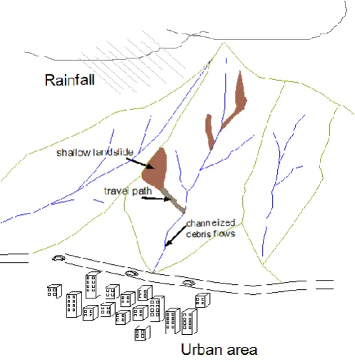
2.1 Shallow landslide schematic representation. Taken from Sidle and Ochiai, 2006
2.2 Shallow landslide within the context of landslide risk
2.3 Typical soil-water retention curve showing approximate locations of residual water content θr, saturated water content θs, and air entry value b
2.4 Shear strength surface in space of net normal stress, suction stress, and shear stress
2.5 Projection of shear strength surface shown in Fig. 2.3 on shear stress-net normal stress plane.
2.6 Schematic representation of the force balance on a rigid block on an inclined plane
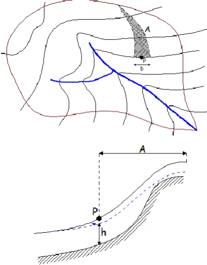
2.7 Sketch of an elementary drainage area: (top) planar view and (bottom) longitudinal section
2.8 Diagrams of the development of soil moisture patterns (top 30 cm) showing the different degrees of connectivity between February (dry state) and September (wet state) 1996 at the Tarrawarra catchment. Contours show surface topography at 1 m intervals
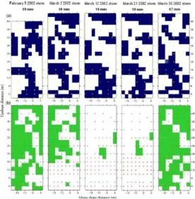
2.9 Map of the location of above median soil moisture (blue, a) and subsurface saturation (green, b) for 5 storms in 2002 at the Panola hillslope Georgia, USA, identifying the disparity between subsurface saturation and surface soil moisture. Yellow dots in (a) represent soil moisture measurement locations; red dots in (b) show the positions of maximum rise wells for water table detection. Taken from Tromp Van Meerveld and McDonnell (2005)
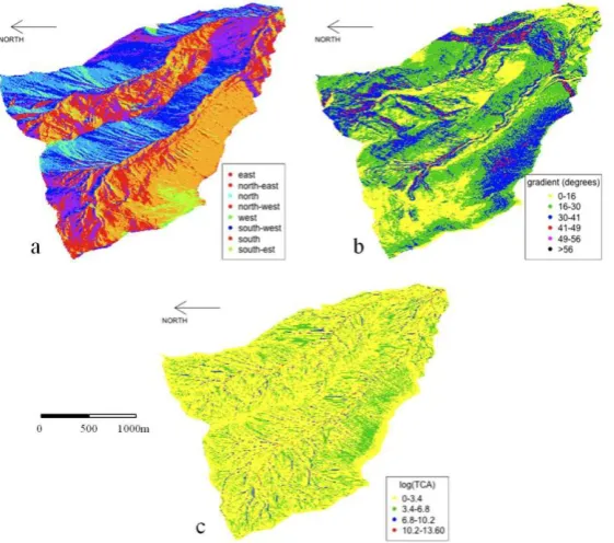
3.1 Maps of topographic drainage directions (a), local slope tan (b), and upslope contributing area A (c) of the Salei catchment. The upslope contributing area is mapped as the natural logarithm of the area in m2
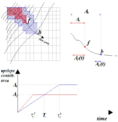
3.2 An example of time-variable upslope contributing area. Regardless of their steady-state upslope contributing area A, during a rainfall event the effective (time-variable) upslope contributing area, Af(t), of a point f located upslope may be larger than the effective
(time-variable) upslope contributing area, Ab(t), of a point b located downslope along the
same flow path
xiv
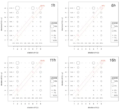
topographic surface gradient (zb). Directions are coded with numbers ranging from 1
(east direction) to 8 (south-east direction), going counterclockwise. The percentages in the left and bottom inside margins of the plots represent the percentage of points characterized by a given value of water table drainage direction and topographic surface drainage direction, respectively
3.5 2-dimensional transect of Salei catchment and simulated water-table level by BEq model. The red line in panel (a) shows the position of the transect reported in panel (b). Low water storage deficit is observed near topographic hollows at the foot slope and where the irregular downslope topography prevents the free water drainage
3.6 Spatial patterns of the traditional “non dispersive” topographic index TWI (a), dynamic topographic index TWId (b), traditional “dispersive” topographic index TWI
mf
(c), smoothed dynamic topographic index TWI*d (d), and BEq-derived water table levels (e).
The maps show in gray the points lower than the 75th percentile and in black the points higher than the 75th percentile of the individual cumulative distribution functions
3.7 On the left, temporal evolution of Spearman’s rank correlation coefficient ρ between simulated water table level and traditional non-dispersive topographic index, TWI (blue), dynamic topographic index, TWId (red), smoothed dynamic topographic index, TWI
* d
(black), and dynamic index where the DWI is used to describe the local drainage, TWIDWId (green). On the right, the role played by the low-pass filter on the terrain indices
performance
3.8 Bar plots showing the ability of the different terrain indices to reproduce connected “wetter” areas. The rightmost bars-block represent the number of isolated “wetter” clusters provided by the five (TWI, TWI*, TWImf, TWId, TWI
*
d) terrain indices (bars) and
the BEq model (dashed line). The first, second, third and fourth bars-blocks represent the 1st quantile, 2nd quantile, mean, and 3rd quantile values of the individual cumulative distribution functions of the “wetter” cluster sizes
3.9 Conceptual representation of the threshold effect on the value of upslope contributing area at the hillslope/channel transition of digitized watersheds. The point inside the topographic hollow shows a value of upslope contributing area A much higher than a point located one pixel upslope
4.1 Irregular bedrock surface vs regular ground surface at the Panola hillslope (a), and soil depth variability (b)
4.2 Flow chart of the cellular automata model. The stress is propagated until no new unstable locations are generated. The final FS configuration gives an estimation of the most likely hillslope portion to be affected by landslide activation
xv
patches of transient saturation (perched water table), the yellow, grey and brown colors identify variably unsaturated soil conditions. Flow is concentrated in the mid-slope which exhibits the highest pore pressure values
4.4 Maps of pore pressure at the soil bedrock interface of the original 13° Panola hillslope (first row), and the modified 20° and 30° Panola hillslopes (second and third rows, respectively) for the long-rainfall event. Maps of pore-pressure are quite similar during the first stage of rainfall (the maps of 1st hour and 4th hour are showed in the first and second columns, respectively), while the overall inclination significantly affects the dynamic of pore pressure in the second stage of rainfall (the maps of 9th hour and 10th hour are showed in the third and fourth columns, respectively) when lateral flow becomes relevant
4.5 Saturated area and pressure head response for the long-rainfall event. (a) Temporal evolution of saturated area at the soil-bedrock interface of the original 13° and modified 20° and 30° Panola hillslopes during the long-rainfall event. (b) Dynamics of the mean value of positive pressure head versus percentage of saturated area at the soil-bedrock interface for the three analyzed Panola hillslope angles. (c) Temporal evolution of the variance σ 2 of the values of pressure head recorded at the soil-bedrock interface for the three slope angles investigated
4.6 Maps of pore-pressure at the soil-bedrock interface of the modified 30°-Panola hillslope during the short-rainfall (top) and long-rainfall (bottom) events. Patterns of pore pressure are similar when the same value of cumulative rainfall has been achieved
4.7 Temporal patterns of unstable locations generated by the cellular automaton (CA) model for four different values of λ (0.2, 0.4, 0.6, and 0.8 on the first, second, third and fourth row, respectively). The long-rainfall event case (I=6.25 mm/h, D=9h) is here shown. In red are the points classified unstable by the infinite slope stability model (Equation 4.5). The black points are the ones that become unstable when the driving forces of the destabilized locations are redistributed to the neighboring cells (Equation 4.6). Rapid failure propagation is observed for high values of λ (λ=0.6 and λ=0.8) during the second stage of rainfall event (i.e., after 5 hours from rainfall beginning)
4.8 Cumulative rainfall against % of unstable area provided by the CA model for all the rainfall events analyzed. Instability spread very quickly when a cumulative rainfall of 30-35 mm was exceeded
4.9 A comparison between the hydrological behavior of the “irregular” Panola hillslope and a “regular” planar hillslope. Both slopes received an input of 6.25 mmh-1
xvi
preventing the free downslope drainage) resulting in complex patterns of instability (Figure 4.7). The vertical dimensions in panels (b) and (d) are exaggerated differently
5.1 A flow chart depicting the coupled saturated/unsaturated hydrological model developed in this Chapter
5.2 The concept of hydrological connectivity. Lateral subsurface flow occurs at point (x,y) when this becomes hydrologically connected with its own upslope contributing area A(x,y) (b)
5.3 i(z) and i(z) are, respectively, the initial water content and the initial suction head
vertical profiles. wt(z) and wt(z) represents the linear water content and suction head
vertical profiles associated with zero-suction head at the soil-bedrock interface
5.4 Catchments case study. The map shows the location of the three catchments, and the landslide distribution (polygons inside the catchments)
5.5 Patterns of Return period TR (years) of the critical rainfalls for shallow landslide
triggering (i.e., FS≤1) and associated levels of landslide susceptibility
5.6 Modelled local rainfall intensity-duration (I-dc) thresholds for shallow landslide initiation at the three investigated catchments, and experimental I-d that triggered debris flow in some alpine catchments (of the Dolomities) similar to our study area
5.A1 The balls in the three dimensional space represent the differences betweentwt computed
with HYDRUS-1D and twt computed with the simplified infiltration model (presented in Section 5.2.1) for 50 scenarios obtained by combining different values of soil thickness, rainfall intensity, and initial pore pressure profile
A.1 (a) The geometry of the real Panola hillslope, (b) the topography of Little Panola, and (c) the 11:1 scale model of the Panola hillslope
A.2 The rainfall simulator mounted on Little Panola (a). Two independent rainfall systems (b) allowed to reproduce a 22 mmh-1 and a 47 mmh-1 constant rainfall intensity event A.3 Location of pore-water pressure transducers at the “soil/bedrock interface” of Little
Panola
A.4 Bedrock topography at different slope inclination on a representative upslope transect across the hillslope (left). Map of contributing area based on bedrock topography for the three slope angle analyzed (right)
A.5 Experimental pore-water pressure measurements at the soil-bedrock interface of the 6 -configuration of Little Panola
A.6 Experimental pore-water pressure measurements at the soil-bedrock interface of the 23 -configuration of Little Panola
xvii
different times form the onset of rainfall along the transect A-A’. Pore-water pressures are measured at the soil/bedrock interface
A.9 Numerical experiments exploring the effect of the downslope boundary condition and the shape of the subsurface topography on pore-water pressure dynamics at the soil/bedrock interface of Little Panola
xix
2.1 Landslide classification (Varnes, 1978)
2.2 A list of the major efforts of the last 30 years to produce more realistic terrain indices from digital elevation models
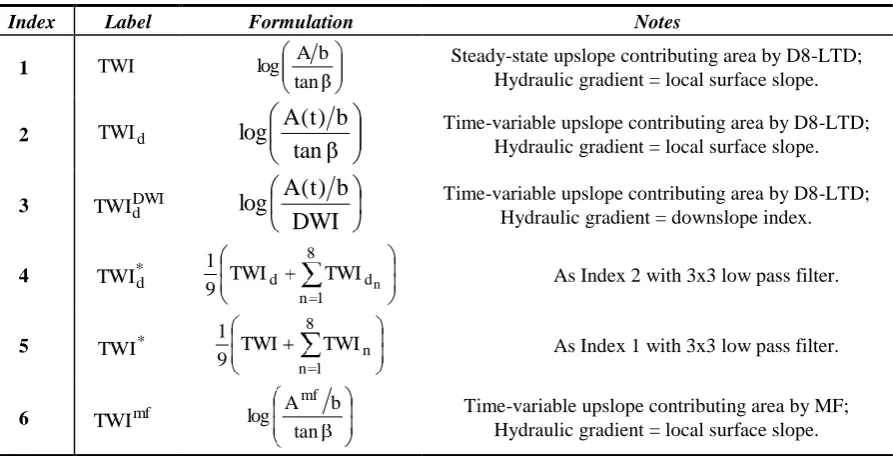
3.1 The six terrain-based indices defined in this study and their major features
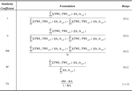
3.2 An overview of the applied similarity coefficients (Approach I) and their theoretical range. The case of the traditional dispersive TWI index is here reported
3.3 Similarity coefficients between reclassified binary maps of wetness indices (TWI, TWImf, TWId, TWI
*
d,) and simulated water table depth (or storage deficit) by BEq model with
zk=75th percentile of the individual cumulative distribution functions. Values in bold
represent the best index at a given rainfall-hour
3.4 Similarity coefficients between reclassified binary maps of wetness indices (TWI, TWImf, TWId, TWI
*
d,) and simulated water table depth (or storage deficit) by BEq model with
zk=25th percentile of the individual cumulative distribution functions. Values in bold
represent the best index at a given rainfall-hour
4.1 Average soil thickness z and hydrological parameters of the soil and saprolite bedrock layers of Panola Hillslope (from Hopp and McDonnell, 2009)
4.2 The hillslope angles and rainfall event features used in the virtual experiments. I = rainfall intensity; D = rainfall duration.
5.1 Hydraulic and mechanical soil-parameters relative to the three investigated catchments 5.2 Percentages of slope-stability categories in terms of catchment area and observed
landslide area in each range of critical rainfall frequency (i.e., return period TR) or level of shallow landslide susceptibility
xxi
This research tries to fill a gap between two very different scales of enquiry: the local (i.e. hillslope) scale, where detailed investigations are possible but difficult to generalize over large areas, and the landscape (i.e., catchment) scale, where representation of the physics is minimised, the resolution in space and time is maximised, and the focus is upon predicting emergent properties rather than system details. Specifically, this Thesis focused on an aspect of the geosciences that is of critical current concern: the representation of the interface between hydrological response and geomorphic processes, notable mass movements. At present there remains a great difficulty at this interface: detailed geotechnical and hydrological studies of mass movements reveal exceptionally complex interlinkages between water and the surface sediment mass, notably dynamically at the onset and during mass release; but these kinds of studies are only possible with a very detailed description of the three-dimensional structure of the porous media and its hydrological and mechanical response during (and after) rainfall events. Such analyses are feasible but tend to result in analyses that are restricted in terms of geographical generalisation. On the other hand, approaches that apply to larger spatial scales tend to over-simplify the representation of critical failure processes, such as in the assumptions that infinite slope stability analysis can be applied to failures that are finite in their slope length, or that upslope contributing area can always act as a surrogate for the hydrologic response at a point in the watershed.
The innovative element in this research lies on the assessment of rainfall-induced shallow landslide occurrence over large spatial scales, whilst accepting that shallow landslides triggering may be influenced by processes that operate over much smaller scales. Specifically, this Thesis focuses upon connection by subsurface flow pathways. New model approaches that incorporate connectivity are required to address the findings of field hydrologists. Thus, this Thesis starts from the understanding of small-scale hydrological processes to develop a large-scale topographic index-based shallow landslide model that includes the concept of subsurface hydrological connectivity.
- 1 -
Introduction
1.1 General introduction and problem statement
Landslides represent a major threat to human life, property and constructed facilities, infrastructure and natural environment in most mountainous and hilly regions of the world. A landslide is defined as "the movement of a mass of rock, debris, or earth down a slope" (Cruden, 1991). Failure of a slope occurs when the force that is pulling the slope downward (gravity) exceeds the strength of the earth materials that compose the slope. Landslides can move slowly (millimeters per year), or can move quickly and disastrously, as is the case with shallow landslides.
The term shallow landslide is used to describe movements by which material is displaced over a discrete slip surface close to the land surface. Shallow landslides are particular important in terms of natural hazard, as they often translate into rapidly moving debris flows (Iverson et al.,1997) that may affect human life and properties (Olshansky,1990; Schuster, 1996; Sidle and Ochiai, 2006; Keefer and Larsen, 2007).
In the last century, Europe has experienced the second highest number of fatalities and the highest economic losses caused by landslides compared to other continents (Figure 1.1): 16,000 people have lost their lives because of landslides and the material losses amounted to over $1700 million in Europe during the 20th century.
- 2 - Within Europe, Italy has been the country that has suffered the greatest human and economic losses due to landslides. In Italy, while about 500 people have been killed by landslides over the past 25 years, the total number of persons impacted is 50 times that number.
Shallow landslides may be triggered by different factors, either natural or related to human activities. Among natural factors, rainfall is certainly one of the most frequent causes of landslides occurrence. Intense storms with high-intensity, long-duration rainfall have great potential to trigger rapidly moving landslides and have been documented as one of the major cause for shallow landslide triggering (Anderson and Sitar 1995; Iverson et al. 1997; Montgomery and Dietrich, 1994; Van Asch et al., 1996; Terlien, 1998; Ng and Shi, 1998; Iverson, 2000; Sidle and Onda, 2004; Malet et al., 2005). Significant examples are provided by multiple shallow phenomena periodically occurring in New Zealand (Crozier, 2005), Washington (Baum et al., 2005), California (Godt et al., 2008), Brazil (Ahrendt and Zuquette, 2003), Japan (Matsushi et al., 2006), Italy (Del Prete et al., 1998). In Italy, about 70% of landslides are triggered by precipitation and rainfall infiltration in a mantle of colluvial soils (Figure 2.1).
Figure 1.2. Landslide triggers in Italy. (Source: CNR-GNDCI AVI Database of areas affected by landslides and floods in Italy)
Rainfall infiltration reduces the soil-shear strength by decreasing the positive effect on stability due to negative pore pressure (Bishop, 1959; de Campos et al., 1994; Godt et al, 2009) or by increasing the positive pore pressure values (e.g., Terzaghi, 1943). The failure surfaces may form within the weathered material (e.g., Lu and Godt 2008; Hawke and McConchie, 2009), but often correspond to the point of contact between the soil and the less permeable bedrock, where a temporary perched water table could develop (e.g., Dietrich et al., 2007; Baum et al., 2010).
- 3 - Guzzetti et al., 2008). An empirical threshold defines the rainfall, soil moisture, or hydrological conditions that, when reached or exceeded, are likely to trigger landslides (Reichenbach et al., 1998). Rainfall intensity-duration thresholds for the possible occurrence of landslides are defined through the statistical analysis of past rainfall events that have resulted in slope failures, and can be classified based on the geographical extent for which they are determined (i.e., global, national, regional, or local thresholds), and the type of rainfall information used to establish the threshold (Guzzetti et al., 2007, 2008).
The second approach to evaluate the dependence of landslide occurrence on rainfall events relies on the use of mathematical models based on physical laws to understand the physical processes controlling slope instability (Montgomery and Dietrich, 1994; Wilson and Wieckzorek, 1995; Wu and Sidle, 1995; Iverson, 2000; Borga et al., 2002; Crosta and Frattini, 2003; Simoni et al. 2008). The mathematical models employed span a broad spectrum from relatively simple “pipe and pot” models to parsimonious topographic-index based models to complex, three-dimensional (3D), variably-saturated flow models based on Richards’ equation.
Process-based models rely upon the understanding of the physical laws controlling slope instability. 3D finite element Richards’ equation solvers provide a complete description of the pore pressure fields in saturated/unsaturated soil. However, the 3D Richards’ equation is highly non-linear and requires the solution of extremely large systems of equations even for small problems (Paniconi et al., 2003). Moreover, the parameterization and calibration of these models is often cumbersome due to the small amount and low accuracy of the available data (Hilberts, 2006).
Topographic wetness index-based models have gained wide use to describe the hydrological control on the triggering of rainfall-induced shallow landslide for the assessment of landslide hazard at regional scale (Montgomery and Dietrich, 1994; Wu and Sidle, 1995; Borga et al., 2002; Iida, 1999; Rosso et al., 2006; Claessens et al., 2007; Casadei et al., 2003). SHALSTAB (Montgomery & Dietrich, 1994) is an example of such a models, where the water table thickness above the soil-bedrock interface is calculated from a steady-state mass balance and it is expressed as a function of the traditional topographic index TWI (O’Loughlin, 1986) given by the ratio between specific upslope contributing area A/b (i.e., upslope contributing area, A, per unit contour length, b) and local slope angle tan (TWI=A/b∙tan ).
- 4 - (that will be widely discussed in Chapter 2) were added to the list of models capable of
assessing landslide susceptibility over large areas.
1.2 Motivation and Thesis objectives
Despite the considerable progress in recent decades, catchment-scale shallow landslide models still consider runoff generation and contributing area variability as a continuum. The details of subsurface hydrological processes remain rudimentary in the numerical structure of most slope stability models and there are still many unanswered questions in the dynamics of pore-water pressure generation related to landslide initiation (e.g., Iverson et al., 2000). Almost all such models assume that the soil-bedrock interface is a simple topographic surface paralleling the soil surface. As a result, none of the slope stability models used to assess landslide susceptibility and hazard at the catchment scale have yet included an important new conceptual element derived from the hillslope hydrology literature: the filling and spilling of water perched at the soil-bedrock interface. Indeed the importance of moisture dynamics at the soil-bedrock interface has been widely acknowledged in hillslope hydrology (e.g., Weiler et al., 2005). Recent hydrological analyses by several groups in several different hydrogeological settings (e.g., Spence and Woo, 2003; Buttle et al., 2004) have shown that filling and spilling of microtopographic depressions in the bedrock topographic surface control the development and connectivity of patches of positive pore pressure, and that hydrological connectivity (the condition by which disparate regions on the hillslope are linked via subsurface water flow, Stieglitz et al. 2003) is a necessary condition for lateral subsurface flow to occur at a point (e.g., Tromp van Meerveld and McDonnell, 2006b, Graham et al., 2010; Spence, 2010).
For the hillslope hydrologist, these patches and their downslope connectivity, form the precondition for resultant subsurface stormflow (Tromp van Meerveld and McDonnell, 2006a). This behavior is now viewed as dominant subsurface stormflow delivery mechanism whereby the existence of a threshold relationship between rainfall amount and hillslope outflow appears to be a common property of hillslope drainage (see review in Weiler et al., 2005). For the slope stability modeler, these patches appear to be a key, unstudied part of the landslide initiation process with potential first order hydrologic control on where a slip surface might be found.
Lack of, or only intermittent, connectivity of subsurface flow systems invalidates the assumptions built into the TWI theory (i.e., the variable – and continuum - contributing area concept originally proposed by Hewlett and Hibbert, 1967). However, until now catchment-scale shallow landslide models have failed to include a connectivity component for subsurface flow paths.
- 5 - implicitly account for hydrological connectivity. However, these models are commonly applied at grid-resolution coarser than those that are likely to control connectivity and landslide occurrence (Lane et al., 2009). The reasons for such coarser resolution are twofold. Firstly, physically-based numerical models are exceptionally demanding in terms of parameterization (Merritt et al., 2003). The information demand for model calibration often exceed available data, and the models are rarely parsimonious with respect to the data available to determine them. The second reason lies on the computational difficulty of running such models with time steps that are small enough to capture the dynamics of shallow landsliding coupled to the need to understand the landsliding process over potentially large spatial extents. It is therefore required to make simplifying assumptions related to hydrologic response (Loague et al., 2006) in order to include a connectivity component in catchment-scale shallow landslide models.
This is what has been done by Lane et al. (2004) to represent surface hydrological connectivity. Lane et al. (2004) developed a network index as an index to describe the level of catchment-averaged saturation required for a saturated point in the hillslope to be hydrologically connected to the drainage network along the complete hydrological flow path that connects the point to the drainage network. The network index of a point is the lowest value of the topographic index along the flow path that connects it to the drainage network by surface overland flow.On its own, TWI does not describe connectivity, but Lane et al. (2004) argued that the spatial arrangement of TWI provide a measure for overland flow connectivity as locally deep water tables (from the ground surface) reduce the propensity to overland flow and increase the probability of water infiltration into the soil. Therefore, the network index treatment has two important hydrological effects: (a) it only allows saturated areas to connect to the hydrological network when there is full saturation along the associated flow path; and (2) overland flow associated with unconnected but saturated zones is assumed to remain within the catchment and to contribute to a reduction in the catchment-averaged saturation deficit.
By considering that connectivity of patches of transient saturation from a location to another on the hillslope depends upon the balance between processes that encourage lateral connection along a flow path and those that disconnect a flow path (e.g., bedrock depressions - Freer et al., 2002; Tromp van Meerveld and McDonnell, 2006a; Hopp and McDonnell, 2009 - and dry soil-moisture conditions - Western et al., 1999 and 2001), an approach similar to the one presented in Lane et al. (2004) should also be applicable to represent subsurface hydrological connectivity (Lanni et al. 2011).
This Thesis exactly deals with the interaction between hydrological processes, notably in terms of subsurface hydrological connectivity, and shallow landslide initiation.
- 6 - scale.
At the hillslope scale, detailed hydrological studies reveal exceptionally complex interlinkages between water and the surface sediment mass, notably dynamically at the onset and during mass movement; these kinds of studies are only possible with a very detailed description of the three-dimensional structure of the sediment mass and its hydrological response during events. Such analyses are feasible but tend to result in analyses that are restricted in terms of geographical generalization; at the landscape (i.e., catchment) scale, shallow landslide modeling tends to over-simplify the representation of hydrological processes by failing to include important controls (such as hydrological connectivity) on both pore-water pressure dynamics and, therefore, landslide triggering mechanisms.
Thus, the innovative element in this research lies on the assessment of subsurface hydrological connectivity over large spatial scales, potentially 10s or 100s of km2, whilst accepting that shallow landslide initiation and subsurface hydrological connectivity may be influenced by processes that operate over much smaller scales (≤10 m). The model aims to provide more realistic assessments of when shallow landslides may occur and where landsliding may occur at the catchment scale to support decision makers in developing more accurate land-use maps and landslide hazard mitigation plans and procedures. To achieve this aim, the three following interrelated objectives - that move from physical understanding, processes conceptualization, and model (re)formulation of near-surface flow dynamics and landslide triggering mechanisms – will be pursued by this Thesis:
Objective 1. Formulate a new topographic wetness index to include the relative role of upslope and downslope topography and (at least partially) overcome the limitations found in traditional topographic indices (i.e., the steady-state assumption for subsurface flow, and the hypothesis that subsurface hydraulic gradient is locally parallel to the gradient of surface topography).
Objective 2. Address the role played by bedrock topography on subsurface pore-water pressure dynamics and resulting hydrological connectivity. Specifically, it is tested the hypothesis that small-scale variability of soil depth and subsurface topography control the degree of drainage pathway connectivity. To meet the objective, the well characterized Panola hillslope hydrological research site (Freer et al., 2002) is used as a virtual laboratory to explore how soil depth, slope inclination and other factors conspire to trigger shallow landslides.
- 7 - 1.3 Thesis outline
Following this introductory chapter, this Thesis comprises of five more chapters dealing with the objectives mentioned above. In Chapter 2, a comprehensive literature review of shallow landslide processes is presented. It documents past research on hydrological processes leading to shallow landslides. The chapter covers various modeling approaches with particular emphasis on those used to assess shallow landslide occurrence at the catchment-scale. Moreover, Chapter 2 will introduce the concept of hydrological connectivity and its contribution to understanding runoff-dominated geomorphic systems. Chapter 3 deals with Objective 1. It is shown that the new topographic wetness index is able to better reproduce spatial patterns of wetness areas as provided by a distributed, physically-based, Boussinesq Equation solver (BEq) than traditional topographic wetness indices.
Chapter 4 focuses on physical understanding of hydrological processes operating at the hillslope scale (Objective 2). The work builds upon the work of Hopp and McDonnell (2009) where they used the 3D Richards’ equation solver, Hydrus 3-D (Simunek et al., 2006), to quantify patterns of pore pressure development and 3D flow in porous media. Moreover, a
simplified cellular automata model is developed to simulate the spatial propagation of destabilized area after failure initiation.
Chapter 5 deals with Objective 3 presenting the new catchment-scale shallow landslide model. The model is applied to three catchments in the central Italian Alps for which a detailed landslides inventory is available.
In Chapter 6, a synthesis of the research is presented. The results obtained are summarized, and evaluated. Limitations of the methods are presented, together with suggestions for future model improvements and research needs.
- 9 -
Literature review
2.1 Introduction
A broad understanding of various topics in hydrological and geotechnical science and modelling technology was required to complete the studies presented in this thesis and it is important to review each of them thoroughly. The first part of this Literature review (Sections 2.2 and 2.3) gives a brief description of water-induced shallow landslide processes. Particular attention is paid to transient infiltration into saturated/unsaturated soil, effective stress in unsaturated soils, shear strength of hillslope soils, and transient stability of infinite slopes. Subsequently, common approaches of modelling shallow landslides at the catchment scale are reviewed (Section 2.4).
The second part of this Chapter (Section 2.5 and 2.6) focuses on the use of digital terrain analysis in hydrological and shallow landslide modeling. Algorithms that have been developed to compute topographic indices are reviewed and discussed (Section 2.5). The concept of hydrological connectivity (i.e., the condition by which disparate regions on the hillslope are linked via subsurface water flow) is introduced in Section 2.6, and a recent attempt to include a connectivity component in topographic index-based hydrological models is also presented.
2.2 General landslide feature
The term landslide is generally used to denote a downslope movement of mass of earth, debris or rock down a slope due to the action of external forces such as rainfall, snowmelt, volcanic eruption, earthquakes, anthropogenic activities etc.
- 10 -
Table 2.1. Landslide classification (Varnes, 1978)
________________________________________________________________________________________ ________________________________________________________________________________________ Type of movement Type of material
________________________________________________________________________________________
Bedrock Soil
_________________________________________________
Coarse Fine
________________________________________________________________________________________
Fall Rock fall Debris fall Earth fall
Topple Rock topple Debris topple Earth topple
Slide Rotational
Rock Slide Debris slide Earth Slide Translational
Spread Rock spread Debris spread Earth spread
Flow Rock flow Debris flow Earth flow
Complex Combination of two or more
A landslide occurs when stresses acting on soil mass on a hillslope exceed the soil-shear strength. It has generally been recognized that these forces are functions of various parameters relating to bedrock geology, lithology, geotechnical properties, rainfall characteristics (intensity and duration), soil-moisture conditions, water table position, and land-use patterns. Additionally, in many cases human interferences are also responsible for triggering the landslides and create the same effects on a slope as a range of natural processes. Some of the common examples of human interferences leading to landslides are changes in land-cover, deforestation, cutting of slopes etc.
2.3 Water-induced shallow landslide processes
Landslides in which the sliding surface is located within the soil mantle or weathered bedrock (typically to a depth from a few decimeters to several meters) are categorized as shallow landslides. A schematic diagram of a shallow landslide is presented in Figure 2.1.
Figure 2.1. Shallow landslide schematic representation. Taken from Sidle and Ochiai, 2006.
- 11 - pressures and therefore reduces the soil-shear strength. Analysis and prediction of stress conditions leading to landslides is largely grounded on Terzaghi’s (1943) effective stress principle for saturated materials. This principle states that the controlling variable for the mechanical behavior of earth materials is effective stress, defined as the difference between total stress and positive pore water pressure. However, this definition may not be appropriate for assessing the state of stress in hillslopes nor completely describe shallow failure of hillside materials under partially saturated conditions since it neglects the effect of unsaturated soil conditions on the soil-shear strength (e.g., Rahardjo et al., 1995; Terlien, 1998; Van Asch et al., 1999; Hornbaker et al., 1997; Mitarai and Nori, 2006). Theoretical and analytical results from a variety of geologic and climatic settings have advanced the hypothesis of shallow slope failure in partially saturated materials (Morgenstern and de Matos, 1975; Wolle and Hachich, 1989; Rahardjo et al., 1996; Collins and Znidarcic, 2004). Godt et al. (2009) reported instrumental observations from a coastal bluff in the Seattle, WA area where a shallow landslide occurred in the apparent absence of positive pore water pressures under partially saturated soil conditions. When rainwater infiltrates through an unsaturated zone, the advancement of the wetted zone near the slope surface may lead to
failure during periods of prolonged rainfall. If the effective cohesion of soil is zero (c′=0), and the slope angle ( ) is greater than or equal to the effective internal friction angle of the soil ( ′), the unsaturated soil slope fails from a loss of apparent cohesion upon saturation of the soil by the infiltrating wetting front. In this case, failure from a reduction in the shear strength because of a rise in the ground water table or the occurrence of a perched water table is unlikely since the slope can only be stable with the shear strength due to the matric suction that fully disappears before saturation is achieved. However, if the slope angle does not exceed the effective friction angle of the soil, slopes are not susceptible to failure from the loss of matric suction since the slopes remain stable without the additional shear strength due to the matric suction; yet the slopes will fail from a reduction in the effective stress in the saturated condition that results in the reduction in the shear strength of soil. When a slope possess an effective cohesion component (c′), and the effective cohesion of the soil is adequate, even a partially saturated slope with a slope angle that is greater than the effective friction angle can remain stable in spite of a complete loss of apparent cohesion. However, even these types of slopes would fail in the saturated condition if an increase in pore pressure reduces the effective stress (Sudhakar, 1996).
- 12 -
Figure 2.2. Shallow landslides within the context of Landslide Risk
The connectivity between upland landslides and stream channels is a very significant factor in the propagation and run-out potential of debris flows. For high magnitude events (i.e., exceptionally heavy rainfall events), debris stored upon hillslopes and within valley floors provides a source of generally unconsolidated sediment that can be entrained and mobilised by channelized debris flows. It follows that the accumulation of unconsolidated debris from numerous shallow landslides over time can provide a large volume of sediment capable of being mobilised in a single episodic channelized debris flow event. Thus, shallow landslides have high potential of causing damage and human losses due to the high velocities in the post-failure phase and the increase in the mobilized volumes during the downhill path. However, prediction of shallow landslide remains a difficult task due to uncertainties regarding hydro-mechanical properties and limited understanding of the underlying triggering mechanisms.
2.3.1 Rainfall infiltration in saturated/unsaturated soil
In the unsaturated zone, the fluid motion is assumed to obey the classical Richards equation (Richards, 1931). The water-mass balance equation for both unsaturated and saturated condition is:
t ) ( z q y q
x
qx y z
- 13 - where [FL-3] is the density of water, qx, qy, qz [LT-1] are fluxes in the x, y, and z directions, respectively; t [T] is the time, and θ [L3L-3] is the volumetric water content. Darcy’s law can be generalized to unsaturated fluid flow problems by considering hydraulic conductivity as a function of suction head (i.e., negative pressure head) (Buckingham, 1907):
z H ) ( k q ; y H ) ( k q ; x H ) ( k
qx x y y z z (2.2)
where [L] is matric suction head, and k( ) [LT-1] is the unsaturated hydraulic conductivity function. In the absence of an osmotic pressure head, the total head H [L] in unsaturated soil is the sum of the matric suction head and the elevation head Z [L]: H= +Z. Thus, substituting Eq. (2.2) into Eq. (2.1) with the hypothesis of constant water density leads to:
t 1 z ) ( k z y ) ( k y x ) ( k
x x y z (2.3)
The term tof Eq. (2.3) can be rewritten in terms of the matric suction head by applying the chain rule:
t
t (2.4)
where is the soil water capacity [L-1] (i.e., the slope of the relationship between volumetric water content and suction head):
) (
C (2.5)
Substituting Equations (2.4) and (2.5) into Eq. (2.3), a governing equation for transient unsaturated flow may be written as:
t ) ( C 1 z ) ( k z y ) ( k y x ) ( k
x x y z (2.6)
Equation (2.6) is the Richards’ equation. To solve Equation (2.6) mathematical descriptions of the soil water retention curve (SWRC) θ( ) and hydraulic conductivity function (HCF) k( ) are required.
SWRC illustrates the relationship between suction and water content of a soil. Some common terms such as saturated volumetric water content, θs [L3
- 14 -
Figure 2.3. Typical soil-water retention curve showing approximate locations of residual water content θr, saturated water content θs, and air entry value b.
Coefficient of permeability, volume change, pore-size distribution, particle size distribution, water content of soil at any matric suction, can be related to the SWRC directly or indirectly. A complete SWRC consists of drying and wetting curves (Fig. 2.2). The drying curve represents the water desorption of a soil when the matric suction increases while the wetting curve represents the water adsorption when matric suction decreases. A number of equations have been developed to describe the SWRC (Gardner, 1958; Brooks and Corey, 1964; van Genuchten 1980; Fredlund and Xing, 1994).
Among these, van Genuchten model (1980) historically has been widely adopted because of a higher degree of fitting to observed soil retention data. The van Genuchten equation has the following form:
n 1 1
n r
sat r e
) ( 1
1 )
(
S (2.7)
where Se [-] is the relative saturation degree, θ [L3L-3] is the actual water content, [L] is the matric suction head, α [L-1] is a parameter that depends approximately on the water-entry value suction, n [-] is a parameter that depends on the soil pore-size distribution.
HCC illustrates the relationship between suction and hydraulic conductivity. The following Mualem model (1976) is an example of model to predict the hydraulic conductivity k of unsaturated porous media:
2
n 1 1 1 n n e 5
. 0 e
satS 1 1 S
K ) (
- 15 - where Ksat [LT-1] is the saturated hydraulic conductivity.
The Richards equation may also been written in terms of volumetric water content. Following the chain rule, Darcy’s law writes:
x D x ) ( k x ) ( k
qx x x x (2.9a)
y D y ) ( k
qy y y (2.9b)
) ( k x D 1 x ) ( k
qz z z z (2.9c)
where: ) ( C ) ( k
D (2.10)
Where D[L2T-1] is defined as the ratio of the hydraulic conductivity to the soil water capacity and is called hydraulic diffusivity for unsaturated soil.
Substituting Equations (2.9a), (2.9b), (2.9c) into Equation (2.6) leads to:
t z ) ( k z ) ( D z y ) ( D y x ) ( D x z z y
x (2.11)
2.3.2 Shear strength and infinite slope stability model of saturated/unsaturated soil The shear strength of a soil is its resistance to shearing stresses. Shear strength is a measure of the soil resistance to deformation by continuous displacement of its individual soil particles. Shear failure occurs when the stresses between the particles are such that they slide or roll past each other. The Mohr-Coulomb failure criterion describes the state of stress on surfaces where failure occurs (Lambe and Whiteman, 1979; Cernica, 1995). In its simplest form, the criterion may be expressed as:
' tan ) p ( '
c w (2.12)
where [FL-2] is the soil-shear strength, c' [FL-2] is the effective soil cohesion, σ [FL-2] is the normal stress, pw [FL-2] is the pore-water pressure and ’ [°] is the effective angle of internal friction. In Equation (2.12) the term (σ−pw) represents the effective stress for saturated soil (Terzaghi, 1943).
- 16 - shear apparatus, as described in Gan et al. (1988), or modified triaxial apparatus, as described in Fredlund and Rahardjo (1993) and Tarantino and Tombolato (2005).
Bishop (1959) proposed the following single-valued effective stress equation for unsaturated soil: ) p p ( ) p (
' a a w (2.13)
Where σ’ [FL-2
] is the effective stress for unsaturated soil, pa [FL-2] is the air-pore pressure, [-] is the effective stress parameter that depends on the degree of saturation or matric suction. The product (pa-pw) represents the interparticle stress due to suction (suction stress hereafter).
For saturated soil, pa is zero, pw is positive, is equal to one, and Equation (2.13) reduces to Terzaghi’s classical effective stress equation ' ( pw). For completely dry soil, is equal to zero and the effective stress is ' ( pa). For partially saturated soil, is a function of the degree of saturation or matric suction.
Numerous equations which are either related to SWRC or other soil parameters were proposed to predict the effective stress parameter (e.g., Fredlund et al., 1978; Khalili and Khabbaz, 1998; Vilar, 2006). The validity of several forms of was examined by Vanapalli and Fredlund (2002) using a series of shear strength test results for statically compacted mixtures of clay, silt, and sand from Escario and Juca (1989). For matric suction ranging between 0 and 1500 kPa, the following two forms showed good fit to the experimental results:
k
sat
(2.14)
where k is a fitting parameter with experimental data, and:
e r sat
r S (2.15)
The Mohr-Coulomb failure criteria for unsaturated soil incorporating both Bishop’s effective stress and suction stress concept is:
' tan )] p p ( ) p [( '
c a a w (2.16)
Equation (2.16) can be rearranged as:
' tan ) p p ( ' ' c ' c ' tan ) p p ( ' tan ) p ( '
- 17 - where:
' tan ) p p ( ''
c a w (2.17b)
c’ and c’’ represent shear strength due to so called apparent cohesion in unsaturated soil. The apparent cohesion includes the classic cohesion c’ representing shearing resistance arising from interparticle physiochemical forces such as van der Waals attraction, and a second term c’’ describing shear resistance arising from capillarity effects (capillarity cohesion). Physically, capillarity cohesion describes the mobilization of suction stress (pa-pw) in terms of shearing resistance. The concept of suction stress and capillarity cohesion may be better illustrated by plotting Equation (2.17) in the three-dimensional space of Figure 2.4. Net normal stress in this regard is an independent stress state variable and suction stress is a material variable.
Figure 2.4. Shear strength surface in space of net normal stress, suction stress, and shear stress
- 18 -
Figure 2.5. Projection of shear strength surface shown in Fig. 2.3 on shear stress-net normal stress plane.
By substituting Eq. (2.15) in Eq. (2.16) we obtain the following equation for shear strength prediction of unsaturated soil:
' tan )] p p ( )
p [( '
c a w
r sat
r
a (2.18)
where pa [FL-2] is the pore-air pressure.
Generally, slope stability studies are based on the calculation of the factor of safety (FS). For hillslopes, it is common to define FS as the ratio of the resisting force, Fr, to the destabilizing force, Fd, (Graham, 1984):
d r F F
FS (2.19)
- 19 -
Figure 2.6. Schematic representation of the force balance on a rigid block on an inclined plane.
Generalizing for hillslope materials with effective cohesion c’ [FL-2], effective soil frictional angle ’ [ ], volumetric unit weight of soil [FL-3], and slope parallel flow with a water-table thickness h [L] (above the failure surface), the factor of safety for an infinite slope reads:
' tan ) cot (tan Z h tan ' tan ) 2 sin( Z ' c 2
FS w (2.20)
where w [FL-3] is volumetric unit weight of water.
Using the infinite slope stability model (2.20) analysis together with the shear strength of unsaturated soil given by (2.18) and the soil water retention curve (2.7), and assuming that the pore air pressure is atmospheric, the factor of safety of an infinite slope in unsaturated/saturated conditions can be written as:
' tan ) cot (tan z tan ' tan ) 2 sin( z ' c 2
FS w for 0 (2.21a)
' tan ) cot (tan z ) ( S tan ' tan ) 2 sin( z ' c 2
FS e w for 0 (2.21b)
where z [L] is the vertical soil-depth.
2.4 Modelling shallow landslide occurrence at the catchment scale
Shallow landslide modeling is based on a variety of approaches and models. Statistical and physically-based approaches are widely adopted tools in catchment-scale shallow landslide modeling.
2.4.1 Statistical approach
- 20 - factors that are directly or indirectly related to slope failures. Then, it involves an estimate of the relative contribution of these factors in generating slope failures, and classification of land surfaces into zones of different hazard or susceptibility degree (Aleotti and Chowdhury, 1999; Pathak and Nilsen, 2004). Bivariate and multivariate statistical methods are the most commonly used for these predictions. The bivariate statistical analysis is a method that describes the relationship between two variables. In landslide modeling, the bivariate method links each landslide causing factor to the landslide distribution map.
On the other hand, in multivariate statistical analysis, the weighted factors controlling the landslide occurrence indicate a relative contribution of each of these factors to the degree of landslide hazard within a defined land unit. The common property of these analyses is their nature of being based on the presence or absence of stability phenomena within these previously defined land units (Van Westen, 2000). The statistical approach can provide an insight into the multifaceted processes involved in shallow landslide occurrence, and useful assessments of susceptibility to shallow landslide hazard in large areas. However, the results are very sensitive to the data set used in the analysis and it is not straightforward to derive the hazard (i.e. probability of occurrence) from the susceptibility.
2.4.2 Physically-based models
Physically-based models attempt to extend spatially the slope stability models (e.g., the "infinite slope stability method") widely adopted in geotechnical engineering (Wu and Sidle, 1995; Iverson, 2000). To link rainfall pattern and its history to slope stability/instability conditions, physically-based models incorporate infiltration models (e.g., Green and Ampt, 1911; Philip, 1954; Salvucci and Entekabi, 1994). Various approaches have been proposed to predict the accumulation of the infiltrated water into the ground from relatively simple “pipe and pot” models to parsimonious topographic-index based models to complex, 3D variably saturated flow models based on Richards equation.
- 21 - The slope stability component (i.e., the infinite slope stability model) uses this topographic index to analyze the stability of each topographic element.
Assuming that there is no overland flow and no significant bedrock leakage, then the effective precipitation, q [LT-1] (rainfall minus evapo-transpiration), times the upslope contributing area, A [L2], must be the amount of runoff that occurs through a particular grid cell of width b [L] under steady state conditions (Figure 2.7):
sin b h K A
q sat (2.22)
where Ksat [LT-1] is the saturated hydraulic conductivity, h [L] is the water-table thickness above the soil/bedrock interface, and [ ] is the local slope angle.
Equation (2.22) can be rearranged in:
TWI K
q sin b
A K
q h
sat sat
(2.23)
where TWI is the topographic wetness index.
Figure 2.7. Sketch of an elementary drainage area: (top) planar view and (bottom) longitudinal section
Coupling Equation (2.23) with the infinite slope stability model (2.20) leads to the following expression of the factor of safety:
' tan ) cot (tan L TWI K
q tan
' tan ) 2 sin( L
' c 2 FS
sar
- 22 - Several applications show this approach to be capable of capturing the spatial variability of shallow landslides hazard, because of the essential role of topographic control in shallow landsliding. This approach permits uncalibrated predictions and has proven reasonably successful, though there is a tendency for overprediction to occur (Dietrich et al., 2001). In fact, the approach by Montgomery and Dietrich (1994) and Pack et al. (1998) does not account for transient movement of soil water. This simplification can affect model capability of predicting shallow landslide potential because the steady flow condition can be unrealistic in the course of rainstorm.
Unsteady lateral subsurface flow was approached by Okimura and Ichikawa (1985) and Wu and Sidle (1995) by coupling the infinite slope stability model with a groundwater kinematic wave model. Borga et al. (2002) relaxed the hydrological steady-state assumption in topographic-index based shallow landslide models by using a modified version of the quasi-dynamic wetness index developed by Barling et al. (1994). This allowed them to obtain information on the rainfall duration needed to cause slope instability under the assumption that lateral subsurface flow in the saturated zone (i.e., below the water table) occurs simultaneously at any point across the catchment (Grayson et al., 1997). Casadei et al. (2003) linked a dynamic spatially distributed shallow subsurface runoff model accounting for evapotranspiration and unsaturated zone storage to an infinite slope model. To overcome the limitations of a kinematic wave hydrology in gentle and convergent slopes (Hilberts et al., 2004), Troch et al. (2003) and Hilberts et al. (2004) developed the hillslope storage Boussinesq (HSB) equation model. Subsequently, the HSB model has been coupled with the infinite slope stability model by Talebi et al. (2008) to investigate the effect of rainfall and water table variations on hillslope stability.
- 23 - in TRIGRS (transient rainfall infiltration and grid-based regional slope-stability analysis by Baum et al., 2008) which was developed to account for the transient effects of rainfall on shallow landslide initiation. TRIGRS combines an analytical solution for groundwater flow in one vertical dimension with an infinite-slope stability calculation (Savage et al., 2003; Baum et al., 2008). Slope-parallel subsurface flow is simulated by means of the topographic index approach and is used to set the initial soil-moisture condition for numerical simulations.
Three-dimensional hydrological models have been developed to perform physically-based simulations for well characterized field sites. Three-dimensional Richards’ equation solvers provide a complete description of the pore pressure fields in saturated/unsaturated soil. VanderKwaak (1999) developed the Integrated Hydrology Model (InHM) to quantitatively simulate fully coupled three-dimensional variably saturated subsurface flow and two-dimensional surface/channel flow. InHM is capable of simulating the four principal runoff generation mechanisms: Horton overland flow (i.e., infiltration excess), Dunne overland flow (i.e., saturation excess), subsurface stormflow, and groundwater flow. The flexibility of InHM has facilitated successful simulation of hydrologic response for a variety of catchment sizes and hydrologic environments (see VanderKwaak, 1999; Loague et al., 2005; Mirus et al., 2007; Heppner, 2007; Ebel et al., 2007). Simoni et al. (2008) combined the infinite slope stability model with GEOtop (Rigon et al., 2006). GEOtop simulates soil-moisture content and pore pressure evolution resulting from rain infiltration and models subsurface saturated and unsaturated flows, and turbulent fluxes across the soil-atmosphere interface. GEOtop model has been applied within a probabilistic framework in order to account for uncertainties of parameters, and Simoni et al. (2008) have proven to be able to reproduce a real event that occurred in the eastern Italian Alps (Sauris catchment). However, three-dimensional Richards’ equation solvers require the solution of extremely large systems of equations even for small problems (Paniconi et al., 2003). Moreover, the parameterization and calibration of these models is often cumbersome due to the small amount and low accuracy of the available data (Hilberts, 2006). At the catchment scale it is most often necessary to make simplifying assumptions related to hydrologic response (Loague et al., 2006), and topographic-index based models are thus often preferred over more physically-based hydrological models.
2.5 Digital terrain modeling in hydrology: capabilities and limitation
- 24 - Digital terrain modeling has become increasingly popular with powerful analytical functions in geographic information systems (GIS). The results of DEM analyses are particular powerful and useful in many environmental studies such as hydrological modeling (Beven and Moore, 1993), landslide hazard modeling (Montgomery and Dietrich, 1994; Pack et al., 1998; Acharya et al., 2006), soil mapping (Skidmore et al., 1991; Thompson et al., 2001; Scull et al., 2003), land-use change modeling (Verburg et al., 2002; Vanacker et al., 2003), erosion modeling (Mitasova et al., 1996; Cochrane and Flanagan, 1999; Amore et al., 2004).
In hydrological modeling, DEMs are most often used in algorithms to derive slopes, aspects, flow direction, upstream contributing area, etc. In particular, the use of DEMs and topographic attributes extracted from DEMs to simulate water flow paths and spatial patterns of wetness has been a central focus of hydrological modeling ever since the development of the area-slope index in geomorphology (Carson and Kirkby, 1972) and the topographic wetness index (TWI) in hydrology (Kirkby, 1975). These indices have been largely used to infer the water storage in the entire catchment area (e.g. Lamb et al., 1998), the extension of saturated areas (e.g., Grabs et al., 2009), and as general indicators of the influence of topography on soil–water storage dynamics (e.g., McGuire et al., 2005; Tetzlaff et al., 2009a, b) and shallow landslide triggering (e.g., Montgomery and Dietrich, 1994; Borga et al., 2002).
The traditional topographic index (Kirkby, 1975) is normally calculated, by digital terrain analysis, as the natural logarithm of the ratio between the drained area A per unit contour length b, a=A/b, and the slope of the ground surface at the location, tan : TWI = log(a/tan ). Beven and Kirkby (1979) developed the topographic index into a terrain analysis-based hydrologic model (TOPMODEL), which is able to produce a simple relation of soil–water storage (deficit) in a catchment. This model expresses the local storage deficit below saturation by assuming that the major factor affecting the water flow paths is the catchment topography.
When calculating TWI from the DEM, different algorithms and modifications of the original “TOPMODEL” index can be used. The variants of TWI differ in the ways that the specific upslope area a, and local slope tan are computed. Table 2.2 summarizes the algorithms that have been developed to compute the TWI since the early 1980s.
- 25 - eight cardinal and diagonal directions. The accumulated area is then routed to the two cardinal and diagonal directions that are closest to the steepest direction weighted according to their distance from.
Barling et al. (1994) were the first to deal with the problem of the steady-state assumption of flow, arguing that rainfall events are seldom sufficient to bring a hillslope to the steady-state condition. This motivated the development of their quasi-dynamic topographic wetness index with a time-variable upslope contributing area. They showed that the quasi-dynamic index was in closer agreement with the measured pattern of soil moisture storage than the traditional steady-state TWI
Table 2.2. A list of the major efforts of the last 30 years to produce more realistic terrain indices from digital elevation models
________________________________________________________________________________
Improvement
Terrain Index efforts focused No. Authors Year investigate upon Method
________________________________________________________________________________________ 1 Beven and Kirkby 1979 TWI
2 O’Callaghan 1984 a a Single flow direction (D8) and Mark
3 Quinn et al. 1991 a a Multiple flow directions 4 Barling et al. 1994 a a Time-variable upslope area, a(t)
5 Tarboton 1997 a a Infinite possible single-
direction flow path-ways (D∞)
6 Beven and Freer 2001 TWI a Time-variable upslope area, a(t)
7 Borga et al. 2002 TWI a Time-variable upslope area, a(t)
8 Orlandini et al. 2003 a a Path-based method considering
cumulative deviation (D8-LTD)
9 Hjerdt et al. 2003 tan tan Downslope index, DWI 10 Seibert and McGlynn 2007 a a Combination of multiple flow
and D∞ (MD∞)
________________________________________________________________________________________