Integration of Graph Theory and Matrix Approach with Fuzzy AHP for Equipment Selection

JIEM, 2013 – 6(2): 477-494 – Online ISSN: 2013-0953 – Print ISSN: 2013-8423 http://dx.doi.org/10.3926/jiem.403

Integration of graph theory and matrix approach with fuzzy AHP for

equipment selection

Hossein Safari, Alireza Faghih, Mohammad Reza Fathi

1

Faculty of Management, University of Tehran, (Iran)

[email protected]

Received: September 2011 Accepted: March 2013

Abstract:

Purpose:

The main purpose of this paper is proposing a new integrated method to equipment

selection. Proposed approach is based on fuzzy Analytic Hierarchy Process (FAHP) and GTMA

(graph theory and matrix approach) methods that are used for equipment selection.

Design/methodology/approach:

In this paper, a two-step fuzzy-AHP and GTMA methodology is

structured here that GTMA uses fuzzy-AHP result weights as input weights. Then a real case

study is presented to show applicability and performance of the methodology. It can be said

that using linguistic variables makes the evaluation process more realistic. Because evaluation is

not an exact process and has fuzziness in its body. Here, the usage of fuzzy-AHP weights in

GTMA makes the application more realistic and reliable. Proposed approach is applied to a

problem of selecting CNC machines to be purchased in a company.

Findings:

The outcome of this research is ranking and selecting equipment based on Fuzzy AHP

and GTMA techniques. According to this method, the first CNC machine (CNC

) is the best

machine among other machines.

Originality/value:

This paper offers a new integrated method for equipment selection that can be

used in other areas such as supplier selection, facility location selection and etc.

1. Introduction

generated configurations are embedded in an optimal assembly system design problem for simultaneous equipment selection and task assignment by minimizing equipment investment cost. Tuzkaya, Gulsun, Kahraman and Ozgen (2011) proposed an integrated fuzzy multi-criteria decision making methodology for MHESP. The proposed approach is utilized from fuzzy sets, Analytic Network Process (ANP) and Preference Ranking Organization Method for Enrichment Evaluations (PROMETHEE) approaches. Evaluation criteria for the MHESP is weighted by fuzzy-ANP (FANP) approach, then, alternative material handling equipment are evaluated by fuzzy-PROMETHEE (FPROMETHEE) approach. The methodology is applied for a manufacturing company to prove its effectiveness. The rest of the paper is organized as follows: The following section presents a concise treatment of the basic concepts of fuzzy set theory. Section 3 presents the methodology. The application of the proposed method is addressed in Section 4. Finally, conclusions are provided in Section 5.

2. Fuzzy sets and Fuzzy Numbers

Fuzzy set theory, which was introduced by Zadeh (1965) to deal with problems in which a source of vagueness is involved, has been utilized for incorporating imprecise data into the

decision framework. A fuzzy set ̃A can be defined mathematically by a membership function

µ̃A(X), which assigns each element x in the universe of discourse X a real number in the

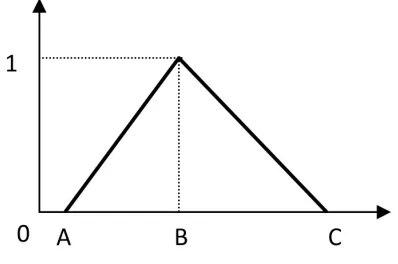
interval [0,1]. A triangular fuzzy number ̃A can be defined by a triplet (a, b, c) as illustrated

in Figure 1.

Figure 1. A triangular fuzzy number ̃A

The membership function µ̃A(X) is defined as

µ̃A(x)=

{

b−a a ≤ x ≤ b x−c

b−c b≤ x ≤ c

0 oterwise

(1)

Basic arithmetic operations on triangular fuzzy numbers A1 = (a1,b1,c1), where a1 ≤ b1 ≤ c1, and

Addition:

A

⊕

A

=

(

a

+

a

,

b

+

b

,

c

+

c

)

Subtraction:

A

⊖

A

=

(

a

−

a

,

b

−

b

,

c

−

c

)

Multiplication: if k is a scalar

K_⊗A1 =

{

(

ka1, kb1, kc1

)

(

)

(4)

Division:

A1Ø A2 ≈

(

a1

c₂, b1

b₂, c1

a₂

)

Although multiplication and division operations on triangular fuzzy numbers do not necessarily yield a triangular fuzzy number, triangular fuzzy number approximations can be used for many practical applications (Kaufmann & Gupta, 1988). Triangular fuzzy numbers are appropriate for quantifying the vague information about most decision problems including personnel selection (e.g. rating for creativity, personality, leadership, etc.). The primary reason for using triangular fuzzy numbers can be stated as their intuitive and computational-efficient representation (Karsak, 2002). A linguistic variable is defined as a variable whose values are not numbers, but words or sentences in natural or artificial language. The concept of a linguistic variable appears as a useful means for providing approximate characterization of phenomena that are too complex or ill-defined to be described in conventional quantitative terms (Zadeh, 1975).

3. Research methodology

In this paper, the weights of each criterion are calculated using fuzzy AHP. After that, GTMA is utilized to rank the alternatives. Finally, we select the best equipment based on these results.

3.1. Fuzzy AHP

This method measures the relativity of fuzziness by structuring the functions of a system hierarchically in a multiple attribute framework. Later on, Buckley (1985) extends Saaty's AHP method in which decision makers can express their preference using fuzzy ratios instead of crisp values. Chang (1996) developed a fuzzy extent analysis for AHP, which has similar steps as that of Saaty's crisp AHP. However, his approach is relatively easier in computation than the other fuzzy AHP approaches. In this paper, Chang's fuzzy extent analysis used for AHP. Kahraman, Cebeci and Ulukan (2003) applied Chang's (1996) fuzzy extent analysis in the selection of the best catering firm, facility layout and the best transportation company, respectively.

Let O = {o1,o2,…,on} be an object set, and U = {g1,g2,…,gm} be a goal set. According to the

Chang's extent analysis, each object is considered one by one, and for each object, the

analysis is carried out for each of the possible goals, gi. Therefore, m extent analysis values for

each object are obtained and shown as follows:

̃ Mgi

1

, ̃Mgi

2

,..., ̃Mgi

m

, i=1,2,..., n

Where M̃gi

j

(j=1,2,3,…, m) are all triangular fuzzy numbers. The membership function of the

triangular fuzzy number is denoted by M(x). The steps of the Chang's extent analysis can be

summarized as follows:

Step 1: The value of fuzzy synthetic extent with respect to the i-th object is defined as:

S_i =

∑

m ̃ M_gj_i⊗[

∑

i=1

n

∑

j=1

m ̃

M_gj_i]−1 ₍₆₎

Where ⊗ denotes the extended multiplication of two fuzzy numbers. In order to obtain

∑

j=1

m

̃

M_g

i

j

We perform the addition of m extent analysis values for a particular matrix such that,

∑

j=1

m ̃ Mgi

j ₌

(

∑

m lj,

∑

j=1

m mj,

∑

j=1

m

uj

)

And to obtain [

∑

i=1

n

∑

j=1

m ̃

M_gj_i]−1 _{we perform the fuzzy addition operation of M̃}

gi

j

(j =1,2,…,m)

values such that,

∑

i=1

n

∑

j=1

m ̃ Mgi

j ₌

(

∑

n li,

∑

i=1

n mi,

∑

i=1

n

Then, the inverse of the vector is computed as,

[

∑

i=1

n

∑

j=1

m ̃ Mgi

j

]

−1

=

(

∑

i=1

n u_i

, 1

∑

i=1

n m_i,

, 1

∑

i=1

n

l_i

)

Where ui, mi, li>0

Finally, to obtain the Sj, we perform the following multiplication:

Si =

∑

m ̃ Mgi

j_⊗[

∑

i=1

n

∑

j=1

m ̃ Mgi

j_]−1 ₌

(

∑

m

lj⊗

∑

n li,

∑

j=1

m

mj⊗

∑

n mi,

∑

j=1

m

uj⊗

∑

n

ui

)

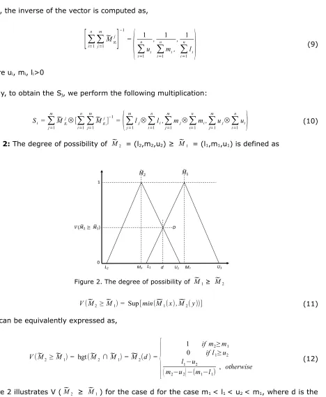
Step 2: The degree of possibility of M̃₂ = (l2,m2,u2) ≥ M̃1 = (l1,m1,u1) is defined as

Figure 2. The degree of possibility of M̃1≥ M̃2

V(̃M2 ≥ ̃M1) = Sup[min(̃M1(x),M̃2(y))] (11)

This can be equivalently expressed as,

V(̃M₂ ≥ ̃M₁) = hgt(̃M₂ ∩ ̃M₁) = ̃M₂(d) =

{

1 if m2≥ m1

0 if l1≥ u2

l₁−u2

(

)

, otherwise (12)

Figure 2 illustrates V (M̃₂ ≥ M̃₁) for the case d for the case m1 < l1 < u2 < m1, where d is the

abscissa value corresponding to the highest cross over point D between M̃₁ and M̃₂,To

compare M̃1 and M̃2, we need both of the values V(M̃1 ≥M̃2) and V(M̃2 ≥ M̃1).

Step 3: The degree of possibility for a convex fuzzy number to be greater than k convex fuzzy

numbers Mi (I=1, 2… K) is defined as

V (_M̃ ≥ M̃₁,M̃₂,…,M̃_k ) =min V(_M̃ ≥ M̃_i), i =1,2,…,k

Step 4: Finally, W=(min V(s1 ≥ sk) min V(s2 ≥ sk),….,min V(sn ≥ sk))T, is the weight vector for

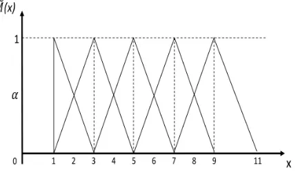
In order to perform a pairwise comparison among the parameters, a linguistic scale has been developed. Our scale is depicted in Figure 3 and the corresponding explanations are provided in Table 1. Similar to the importance scale defined in Saaty's classical AHP (Saaty, 1980), we have used five main linguistic terms to compare the criteria: ‘‘equal importance’’, ‘‘moderate importance’’, ‘‘strong importance’’, ‘‘very strong importance’’ and ‘‘demonstrated importance’’. We have also considered their reciprocals: ‘‘equal unimportance’’, ‘‘moderate unimportance’’, ‘‘strong unimportance’’, ‘‘very strong unimportance’’ and ‘‘demonstrated unimportance’’. For instance, if criterion A is evaluated ‘‘strongly important’’ than criterion B, then this answer means that criterion B is ‘‘strongly unimportant’’ than criterion A.

Figure 3. Membership functions of triangular fuzzy numbers corresponding to the linguistic scale

Linguistic scale triangular fuzzy numbers inverse of triangular fuzzy numbers

Equal Importance (1, 1, 1) (1, 1, 1) Moderate Importance (1, 3, 5) (1/5, 1/3, 1) Strong importance (3, 5, 7) (1/7, 1/5, 1/3) Very strong importance (5, 7, 9) (1/9, 1/7, 1/5) Demonstrated importance (7, 9, 11) (1/11, 1/9, 1/7)

Table 1. The linguistic scale and corresponding triangular fuzzy numbers

3.2. The GTMA method

The step by step explanation of the methodology is as follows:

Step 1: Identifying equipment selection attributes. In this step all the criteria which affect the decision is determined. This can be done by using relevant criteria available in the literature or getting information from the decision maker.

Step 2: Determine equipment alternatives. All potential alternatives are identified.

Step 3: Graph representation of the criteria and their inter dependencies. Equipment selection criterion is defined as a factor that influences the selection of an alternative. The equipment selection criteria digraph models the alternative selection criteria and their inter relationship.

This digraph consists of a set of nodes N = {ni}, with i = 1, 2,...,M and a set of directed edges

E = {eij}. A node ni represents i-th alternative selection criterion and edges represent the

relative importance among the criteria. The number of nodes M considered is equal to the number of alternative selection criteria considered. If a node ‘i’ has relative importance over another node ‘j’ in the alternative selection, then a directed edge or arrow is drawn from node i

to node j (i.e. eij). If ‘j’ has relative importance over ‘i’ directed edge or arrow is drawn from

node j to node i (eji) (Rao, 2007).

Step 4: Develop equipment selection criteria matrix of the graph. Matrix representation of the alternative selection criteria digraph gives one-to-one representation. A matrix called the equipment selection criteria matrix. This is an M in M matrix and considers all of the criteria (i.e. Ai) and their relative importance (i.e. aij). Where Ai is the value of the i-th criteria

represented by node ni and aij is the relative importance of the i-th criteria over the j-th

represented by the edge eij (Rao, 2007; Faisal et al., 2007).

The value of Ai should preferably be obtained from available or estimated data. When

quantitative values of the criteria are available, normalized values of a criterion assigned to the alternatives are calculated by vi/vj, where vi is the measure of the criterion for the i-th

alternative and vj is the measure of the criterion for the j-th alternative which has a higher

measure of the criterion among the considered alternatives. This ratio is valid for beneficial criteria only. A beneficial criteria means its higher measures are more desirable for the given application. Whereas, the non-beneficial criterion is the one whose lower measures are

desirable and the normalized values assigned to the alternatives are calculated by vj/vi.

CSMatrix =

[

A1 a12 a13 a a a1.m

a21 A2 a23 ⋯ ⋯ a2.m

a31 a32 A3 ⋯ ⋯ a3.m ⋮ ⋯ ⋯ ⋯ ⋯ ⋯ ⋮ ⋱ ⋯ ⋯ ⋯ ⋮

a1 a1 a1 ⋯ ⋯ Am

]

(13)

introduced by Cauchy in 1812. At that time, while developing the theory of determinants, he also defined a certain subclass of symmetric functions which later Muir named permanents

(Nourani & Andresen, 1999). The permanent is a standard matrix function and is used in

combinatorial mathematics (Faisal et al., 2007; Rao, 2006). The permanent function is obtained in a similar manner as the determinant but unlike in a determinant where a negative sign appears in the calculation, in a variable permanent function positive signs replace these negative signs (Faisal et al., 2007; Rao, 2006). Application of the permanent concept will lead to a better appreciation of selection attributes. Moreover, using this no negative sign will appear in the expression (unlike determinant of a matrix in which a negative sign can appear) and hence no information will be lost (Rao, 2006).

The per(CS) contains terms arranged in (M+1) groups, and these groups represent the measures of criteria and the relative importance loops. The first group represents the measures of M criteria. The second group is absent as there is no self-loop in the digraph. The third group contains 2- criterion relative importance loops and measures of (M-2) criteria. Each term of the fourth group represents a set of a 3-criterion relative importance loop, or its pair, and measures of (M-3) criteria. The fifth group contains two sub-groups. The terms of the first sub-group is a set of two 2-criterion relative importance loops and the measures of (M-4) criteria. Each term of second sub-group is a set of a 4-attribute relative importance loop, or its pair, and the measures of (M-4) criteria. The sixth group contains two subgroups. The terms of the first sub-group are a set of a 3-criterion relative importance loop, or its pair, and 2-criterion importance loop and the measures of (M-5) criteria. Each term of the second sub-group is a set of a 5-criterion relative importance loop, or its pair, and the measures of (M-5) criteria. Similarly other terms of the equation are defined. Thus, the CS fully characterizes the considered alternative selection evaluation problem, as it contains all possible structural components of the criteria and their relative importance. It may be mentioned that this equation is nothing but the determinant of an M _ M matrix but considering all the terms as positive.

Step 6: Evaluation and ranking of the alternatives, in this step all alternatives are ranked according to their permanent values calculated in the previous step.

per (Cs) =

∏

i=1

M

Ai+

∑

M−1

∑

j=i+1

M

…

∑

M=t+1

M

(aijaji)AkAlAmAnAo… AtAM

+

∑

i=1

M−2

∑

j=i+1

M−1

∑

k=i+1

M

…

∑

M=t+! M

(

)

+

∑

i=1

M−3

∑

j=i+1

M

∑

k=i+1

M−1

∑

l=i+2

M

…

∑

M=t+1

M

(

)

+

∑

i=1

M−3

∑

j=i+1

M

∑

k=i+1

M−1

∑

l=i+2

M

…

∑

M=t+1

M

(

)

∑

i=1

M−2

∑

j=1

M−1

∑

j=i+1

M

∑

l=1

M−1

∑

m=l+1

M−2

… …

∑

m=t+1

M

(

)(

)

∑

i=1

M−4

∑

j=i+1

M−1

∑

k=j+1

M

∑

l=1

M

∑

m=l+1

M

… …

∑

M=t+1

M

(

)

∑

i=1

M−3

∑

j=i+1

M−1

∑

k=j+1

M

∑

l=1

M

∑

m=l+1

M−1

∑

n=m+1

M

…….

∑

M=t+1

M

(

)(

)

+

∑

i=1

M−5

∑

j=i+1

M−1

∑

k=j+1

M

∑

l=1

M−2

∑

m=l+1

M−1

∑

n=m+1

M

… ….

∑

M=t+1

M

(

)

(

)

+

∑

i=1

M−5

∑

j=i+1

M−1

∑

k=j+1

M

∑

l=1

M

∑

m=l+1

M

∑

n=m+1

M

…….

∑

M=t+1

M

(

)

4. A numerical application of proposed approach

The proposed approach is applied in a manufacturing company, located in Qom, Iran. The company wants to purchase a few CNC machines to reduce the work in- process inventory and to replace its old equipment. The high technology equipment make significant improvements in the manufacturing processes of the firms and the correct decisions made at this stage brings the companies competitive advantage. Therefore, selecting the most proper CNC machines is of great importance for the company. But it is hard to choose the most suitable one among the machines which dominate each other in different characteristics. In the application, firstly through the literature investigation and studying other papers that are related to equipment

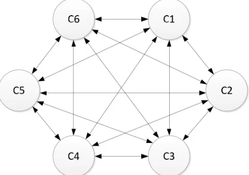
selection, six criteria are selected. These criteria include weight (C1), power(C2), price (C3),

stroke (C4),spindle (C5) and diameter (C6). In addition, there are six alternatives include CNC1,

CNC2, CNC3, CNC4, CNC5 and CNC6. Figure 4 shows the inter relationships between the criteria.

4.1. Fuzzy AHP

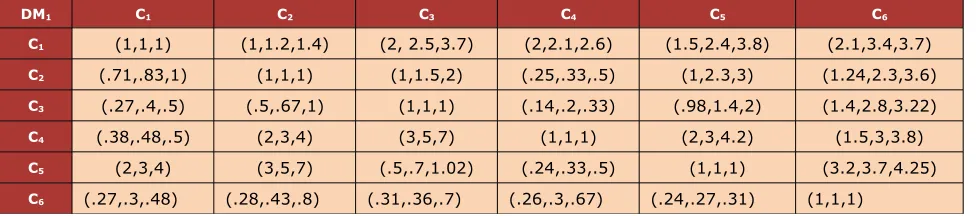
In fuzzy AHP, firstly, the criteria and alternatives’ importance weights must be compared. Afterwards, the comparisons about the criteria and alternatives, and the weight calculation need to be made. Thus, the evaluation of the criteria according to the main goal and the evaluation of the alternatives for these criteria must be realized. Then, after all these evaluation procedure, the weights of the alternatives can be calculated. In the second step, these weights are used to GTMA calculation for the final evaluation. Decision makers from different backgrounds may define different weight vectors. They usually cause not only the imprecise evaluation but also serious persecution during decision process. For this reason, we proposed a group decision based on FAHP to improve pair-wise comparison. Firstly each decision maker (DM), individually carry out pair-wise comparison and you can see them in Table 2, Table 3 and Table 4.

DM1 C1 C2 C3 C4 C5 C6

C1 (1,1,1) (1,1.2,1.4) (2, 2.5,3.7) (2,2.1,2.6) (1.5,2.4,3.8) (2.1,3.4,3.7)

C2 (.71,.83,1) (1,1,1) (1,1.5,2) (.25,.33,.5) (1,2.3,3) (1.24,2.3,3.6)

C3 (.27,.4,.5) (.5,.67,1) (1,1,1) (.14,.2,.33) (.98,1.4,2) (1.4,2.8,3.22)

C4 (.38,.48,.5) (2,3,4) (3,5,7) (1,1,1) (2,3,4.2) (1.5,3,3.8)

C5 (2,3,4) (3,5,7) (.5,.7,1.02) (.24,.33,.5) (1,1,1) (3.2,3.7,4.25)

C6 (.27,.3,.48) (.28,.43,.8) (.31,.36,.7) (.26,.3,.67) (.24,.27,.31) (1,1,1)

Table 2. Pair-wise comparison of first decision maker

DM2 C1 C2 C3 C4 C5 C6

C1 (1,1,1) (2.5,3,3.6) (3.1,3.4,3.6) (2.21,2.6,3.8) (2.33,2.9,3.2) (1.8,2.5,3.21)

C2 (.28,.3,.4) (1,1,1) (.17,.2,.25) (.25,.33,.50) (.33,1.3,1.5) (2.22,3.34,4)

C3 (.27,.29,.3) (4,5,6) (1,1,1) (1.26,1.7,3.2) (2.3,2.8,3.47) (.8,.96,1.3)

C4 (.26,.3,.45) (2,3,4) (.31,.56,.79) (1,1,1) (.33,.5,1) (1.2,1.8,2.6)

C5 (2,3,4) (.3,.56,.8) (.29,.36,.43) (1,2,3) (1,1,1) (2.25,2.5,3)

C6 (.3,.4,.56) (.2,.3,.45) (.77,1.04,1.2) (.38,.56,.83) (.33,.4,.44) (1,1,1)

Table 3. Pair-wise comparison of second decision maker

DM3 C1 C2 C3 C4 C5 C6

C1 (1,1,1) (1,2,3) (.9,1.2,1.9) (3.3,3.9,4.6) (1,2,3) (.33,.5,1)

C2 (.33,.5,1) (1,1,1) (2.3,2.76,3.8) (1.45,3,3.5) (4,5,6) (1.5,1.8,2.11)

C3 (.53,.83,1.1) (.26,.36,.4) (1,1,1) (.14,.17,.2) (2,3,4) (2.6,3.4,4.1)

C4 (.2,.26,.3) (.29,.34,.6) (5,6,7) (1,1,1) (3,4,5) (.2,.5,1.1)

C5 (.2,.26,.3) (5,6,7) (.25,.33,.5) (.2,.25,.33) (1,1,1) (1.05,2.16,2.9)

C6 (1,2,3) (.47,.56,.6) (.24,.29,.38) (.91,2,5) (.34,.46,.9) (1,1,1)

Then, a comprehensive pair-wise comparison matrix is built as in Table 5.

D C1 C2 C3 C4 C5 C6

C1 (1,1,1) (1.5,2.1,2.67) (2,2.37,3.09) (2.51,2.89,3.67) (1.61,2.43,3.35) (1.41,2.13,2.6)

C2 (.44,.55,.8) (1,1,1) (1.16,1.49,2.04) (.65,1.2,1.5) (1.78,2.87,3.5) (1.65,2.5,3.23)

C3 (.36,.51,.65) (1.59,2,2.48) (1,1,1) (.52,.72,1.24) (1.77,2.4,3.16) (1.6,2.39,2.8)

C4 (.29,.37,.42) (1.43,2.11,2.9) (2.77,3.85,4.93) (1,1,1) (1.78,2.5,3.4) (.97,1.77,2.5)

C5 (1.43,2.11,2.9) (2.77,3.85,4.93) (.35,.47,.65) (.48,.86,1.28) (1,1,1) (2.17,2.8,3.4)

C6 (.53,.9,1.34) (.33,.43,.64) (.44,.56,.78) (.52,.96,2.17) (.3,.38,.57) (1,1,1)

Table 5. Fuzzy pair-wise comparison matrix

After forming fuzzy pair-wise comparison matrix, we calculate the weight of all criteria. The weight calculation details are given below. Because of the other calculations are similar for each comparison matrix, these are not given here and can be done simply according the computations below. The value of fuzzy synthetic extent with respect to the i-th object (I = 1,2,...,8) is calculated as

S1= (10.03, 12.9, 16.4) ⊗ (0.0132, 0.0171, 0.02) = (0.1325, 0.2209, 0.3808)

S2= (6.68, 9.61, 12.07) ⊗ (0.0132, 0.0171, 0.02) = (0.0882, 0.1643, 0.2801)

S3= (6.83, 9.02, 11.40) ⊗ (0.0132, 0.0171, 0.02) = (0.0902, 0.1542, 0.2646)

S4= (8.23, 11.6, 15.15) ⊗ (0.0132, 0.0171, 0.02) = (0.1087, 0.1984, 0.3515)

S5= (8.2, 11.08, 14.16) ⊗ (0.0132, 0.0171, 0.02) = (0.1082, 0.1895, 0.3285)

S6= (3.12, 4.23, 6.511) ⊗ (0.0132, 0.0171, 0.02) = (0.0412, 0.0723, 0.1509)

Then the V values calculated using these vectors are shown in Table 6.

(V) S1 S2 S3 S4 S5 S6

S1 - 1 1 1 1 1

S2 0.722 - 1 0.834 0.872 1

S3 0.664 0.945 - 0.779 0.816 1

S4 0.906 1 1 - 1 1

S5 0.861 1 1 0.961 - 1

S6 0.110 0.405 0.425 0.250 0.267

-Table 6. V values result

Thus, the weight vector from Table 5 is calculated and normalized as

4.2. The GTMA method

The weights of the alternatives are calculated by fuzzy AHP up to now, and then these values can be used in GTMA. After calculating the weights, we formed the decision matrix that shows in Table 7. This decision matrix is made by Questionnaire. We used the mathematical mean for forming the aggregate decision matrix.

C1 C2 C3 C4 C5 C6

A1 18.96 0.31 30.61 1.43 16.25 3.72

A2 20.76 0.24 16.33 1.70 11.52 5.93

A3 16.88 0.25 26.55 1.01 15.85 3.72

A4 11.48 0.31 32.87 1.31 12.01 6.21

A5 26.26 0.22 28.68 1.03 12.24 3.48

A6 14.12 0.16 24.58 1.68 9.91 8.22

MAX 26.26 0.31 32.87 1.70 16.25 8.22

Table 7. Decision matrix of GTMA

In the next step, we normalized the decision matrix that shows in Table 8.

C1 C2 C3 C4 C5 C6

A1 0.722 1.000 0.931 0.842 1.000 0.453

A2 0.791 0.779 0.497 1.000 0.709 0.722

A3 0.643 0.806 0.808 0.597 0.975 0.453

A4 0.437 0.989 1.000 0.773 0.739 0.755

A5 1.000 0.710 0.873 0.604 0.753 0.424

A6 0.538 0.508 0.748 0.991 0.610 1.000

Table 8. Normalized decision matrix

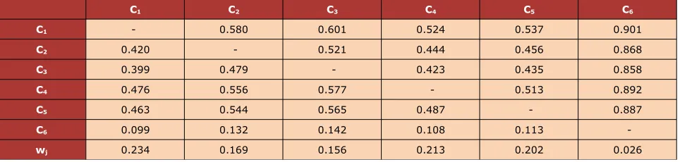
Then, according to GTMA method, we carry out pair-wise comparison with respect to their weight that shows from Table 9 to Table 15.

C1 C2 C3 C4 C5 C6

C1 - 0.580 0.601 0.524 0.537 0.901

C2 0.420 - 0.521 0.444 0.456 0.868

C3 0.399 0.479 - 0.423 0.435 0.858

C4 0.476 0.556 0.577 - 0.513 0.892

C5 0.463 0.544 0.565 0.487 - 0.887

C6 0.099 0.132 0.142 0.108 0.113

-wj 0.234 0.169 0.156 0.213 0.202 0.026

Table 9. Pair-wise comparison of criteria with respect to each other

CNC1 C1 C2 C3 C4 C5 C6

C1 0.722 0.580 0.601 0.524 0.537 0.901

C2 0.420 1.000 0.521 0.444 0.456 0.868

C3 0.399 0.479 0.931 0.423 0.435 0.858

C4 0.476 0.556 0.577 0.842 0.513 0.892

C5 0.463 0.544 0.565 0.487 1.000 0.887

C6 0.099 0.132 0.142 0.108 0.113 0.453

CNC2 C1 C2 C3 C4 C5 C6

C1 0.791 0.580 0.601 0.524 0.537 0.901

C2 0.420 0.779 0.521 0.444 0.456 0.868

C3 0.399 0.479 0.497 0.423 0.435 0.858

C4 0.476 0.556 0.577 1.000 0.513 0.892

C5 0.463 0.544 0.565 0.487 0.709 0.887

C6 0.099 0.132 0.142 0.108 0.113 0.722

Table 11. Pair-wise comparison of criteria with respect to A2

CNC3 C1 C2 C3 C4 C5 C6

C1 0.643 0.580 0.601 0.524 0.537 0.901

C2 0.420 0.806 0.521 0.444 0.456 0.868

C3 0.399 0.479 0.808 0.423 0.435 0.858

C4 0.476 0.556 0.577 0.597 0.513 0.892

C5 0.463 0.544 0.565 0.487 0.975 0.887

C6 0.099 0.132 0.142 0.108 0.113 0.453

Table 12. Pair-wise comparison of criteria with respect to A3

CNC4 C1 C2 C3 C4 C5 C6

C1 0.437 0.580 0.601 0.524 0.537 0.901

C2 0.420 0.989 0.521 0.444 0.456 0.868

C3 0.399 0.479 1.000 0.423 0.435 0.858

C4 0.476 0.556 0.577 0.773 0.513 0.892

C5 0.463 0.544 0.565 0.487 0.739 0.887

C6 0.099 0.132 0.142 0.108 0.113 0.755

Table 13. Pair-wise comparison of criteria with respect to A4

CNC5 C1 C2 C3 C4 C5 C6

C1 1.000 0.580 0.601 0.524 0.537 0.901

C2 0.420 0.710 0.521 0.444 0.456 0.868

C3 0.399 0.479 0.873 0.423 0.435 0.858

C4 0.476 0.556 0.577 0.604 0.513 0.892

C5 0.463 0.544 0.565 0.487 0.753 0.887

C6 0.099 0.132 0.142 0.108 0.113 0.424

Table 14. Pair-wise comparison of criteria with respect to A5

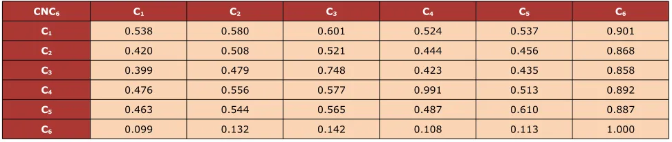
CNC6 C1 C2 C3 C4 C5 C6

C1 0.538 0.580 0.601 0.524 0.537 0.901

C2 0.420 0.508 0.521 0.444 0.456 0.868

C3 0.399 0.479 0.748 0.423 0.435 0.858

C4 0.476 0.556 0.577 0.991 0.513 0.892

C5 0.463 0.544 0.565 0.487 0.610 0.887

C6 0.099 0.132 0.142 0.108 0.113 1.000

Table 15. Pair-wise comparison of criteria with respect to A6

Alternative Permanent matrix

CNC1 10.7761

CNC2 10.0513

CNC3 8.5713

CNC4 10.7022

CNC5 8.7418

CNC6 10.1887

Table 16. Permanent matrix of each alternative

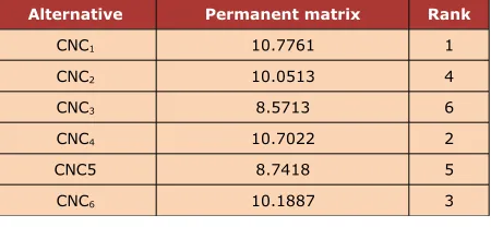
Finally, we rank all machines with respect to their permanent matrix that shows in Table 17.

Alternative Permanent matrix Rank

CNC1 10.7761 1

CNC2 10.0513 4

CNC3 8.5713 6

CNC4 10.7022 2

CNC5 8.7418 5

CNC6 10.1887 3

Table 17. Ranking alternative

According to Table 17, the first CNC machine (CNC1) is the best machine among other

machines.

5. Conclusion

A proper equipment selection is a very important activity for manufacturing systems due to the fact that improper equipment selection can negatively affect the overall performance and productivity of a manufacturing system. In this paper, a two-step fuzzy-AHP and GTMA methodology is structured here that GTMA uses fuzzy-AHP result weights as input weights. Then a real case study is presented to show applicability and performance of the methodology. It can be said that using linguistic variables makes the evaluation process more realistic. Because evaluation is not an exact process and has fuzziness in its body. Here, the usage of fuzzy-AHP weights in GTMA makes the application more realistic and reliable. The proposed model has only been implemented on an equipment selection problem in the company; however, company management has found the proposed model satisfactory and implementable in others equipment selection decisions. As a future direction, other decision-making methods such as fuzzy ELECTRE, fuzzy GTMA and interval GTMA can be used in this area.

Acknowledgement

References

Atmani, A., & Lashkari, R.S. (1998). A model of machine tool selection and operation allocation

in flexible manufacturing system. International Journal of Production Research, 36,

1339-1349. http://dx.doi.org/10.1080/002075498193354

Ayag, Z., & Ozdemir, R.G. (2006). A fuzzy AHP approach to evaluating machine tool

alternatives. Journal of Intelligent Manufacturing, 17, 179-190.

http://dx.doi.org/10.1007/s10845-005-6635-1

Beaulieu, A., Gharbi, A., & Kadi, A. (1997). An algorithm for the cell formation and the machine

selection problems in the design of a cellular manufacturing system. International Journal of

Production Research, 35, 1857-1874. http://dx.doi.org/10.1080/002075497194958

Buckley, J.J. (1985). Fuzzy hierarchical analysis. Fuzzy Sets and Systems, 17, 233-247.

http://dx.doi.org/10.1016/0165-0114(85)90090-9

Chang, D.Y. (1996). Applications of the extent analysis method on fuzzy AHP. European Journal

of Operational Research, 95, 649-655. http://dx.doi.org/10.1016/0377-2217(95)00300-2

Chen, M.A. (1999). Heuristic for solving manufacturing process and equipment selection

problems. International Journal of Production Research, 37, 359-374.

http://dx.doi.org/10.1080/002075499191814

Darvish, M., Yasaei, M. & Saeedi, A.(2009). Application of the graph theory and matrix

methods to contractor ranking. International Journal of Project Management, 27(6), 610-619.

http://dx.doi.org/10.1016/j.ijproman.2008.10.004

Dellurgio, S.A., Foster, S.T., & Dickerson, G. (1997). Utilizing simulation to develop economic

equipment selection and sampling plans for integrated circuit manufacturing. International

Journal of Production Research, 35, 137-155. http://dx.doi.org/10.1080/002075497196028

Faisal, M.N., Banwet, D. & Shankar, R. (2007). Quantification of risk mitigation environment of

supply chains using graph theory and matrix methods. European Journal of Industrial

Engineering, 1(1), 22-39. http://dx.doi.org/10.1504/EJIE.2007.012652

Kahraman, C., Cebeci, U., & Ulukan, Z. (2003). Multi-criteria supplier selection using fuzzy

AHP. Logistics Information Management, 16(6), 382-394.

http://dx.doi.org/10.1108/09576050310503367

Karsak, E.E. (2002). Distance-based fuzzy MCDM approach for evaluating flexible

manufacturing system alternatives. International Journal of Production Research, 40(13),

Kaufmann, A., & Gupta, M.M. (1988). Fuzzy mathematical models in engineering and

management science. Amsterdam: North-Holland.

Kulak, O., Durmusoglu, M.B., & Kahraman, C. (2005). Fuzzy multi attribute equipment

selection based on information axiom. Journal of Materials Processing Technology, 169,

337-345. http://dx.doi.org/10.1016/j.jmatprotec.2005.03.030

Li, S., Wang, H., Hu, S., Lin, Y., & Abell, J. (2011). Automatic generation of assembly system

configuration with equipment selection for automotive battery manufacturing. Journal of

Manufacturing Systems, 30, 188-195. http://dx.doi.org/10.1016/j.jmsy.2011.07.009

Nourani, Y., & Andresen, B. (1999). Exploration of NP-hard enumeration problems by simulated

annealing -the spectrum values of permanents. Theoretical computer science, 215(1-2),

51-68. http://dx.doi.org/10.1016/S0304-3975(99)80002-4

Oeltjenbruns, H., Kolarik, W.J., & Kirschner, R.S. (1995).Strategic planning in manufacturing

Systems-AHP application to an equipment replacement decision. International Journal of

Production Economics, 38, 189-197. http://dx.doi.org/10.1016/0925-5273(94)00092-O

Rao, R.V. (2007). Decision making in the manufacturing environment: using graph theory and

fuzzy multiple attribute decision making methods. London: Springer.

Rao, R.V. (2006). A decision-making framework model for evaluating flexible manufacturing

systems using digraph and matrix methods. The International Journal of Advanced

Manufacturing Technology, 30(11), 1101-1110. http://dx.doi.org/10.1007/s00170-005-0150-6

Saaty, T.L. (1980). The analytic hierarchy process. New York: McGraw- Hill.

Safari, H., Fathi, M.R., & Faghih, A. (2011). Applying fuzzy AHP and fuzzy TOPSIS to Machine

Selection. Journal of American Science, 7(9), 755-765.

Standing, G., Flores, B., & Olson, D. (2001).Understanding managerial preferences in selection

equipment. Journal of Operation Management, 19, 23–37.

http://dx.doi.org/10.1016/S0272-6963(00)00047-4

Sullivan, G.W., Mcdanold, T.N., & Van Aken, E.M. (2002). Equipment replacement decisions and

lean manufacturing. Robotics and Computer-Integrated Manufacturing, 18, 255-265.

http://dx.doi.org/10.1016/S0736-5845(02)00016-9

Tabucanon, M.T., Batanov, D.N., & Verma, D.K. (1994). Intelligent decision support system (DSS) for the selection process of alternative machines for flexible manufacturing systems

(FMS). Computers in Industry, 25, 131-143. http://dx.doi.org/10.1016/0166-3615(94)90044-2

application. Expert Systems with Applications, 37, 2853-2863.

http://dx.doi.org/10.1016/j.eswa.2009.09.004

Van Laarhoven, P.J.M., & Pedrcyz, W. (1983). A fuzzy extension of Saaty’s priority theory.

Fuzzy Sets and Systems, 11, 229-241. http://dx.doi.org/10.1016/S0165-0114(83)80082-7

Wang, T.Y., Shaw, C.F., & Chen, Y.L (2000). Machine selection in flexible manufacturing cell: A

fuzzy multiple attribute decision making approach. International Journal of Production

Research, 38, 2079-2097. http://dx.doi.org/10.1080/002075400188519

Yilmaz, B., & Dagdeviren, M. (2011). A combined approach for equipment selection:

F-PROMETHEE method and zero–one goal programming. Expert Systems with Applications,

38, 11641-11650. http://dx.doi.org/10.1016/j.eswa.2011.03.043

Zadeh, L.A. (1965). Fuzzy sets. Information and Control, 8(3), 338-353.

http://dx.doi.org/10.1016/S0019-9958(65)90241-X

Zadeh, L.A. (1975). The concept of a linguistic variable and its application to approximate

reasoning-I. Information Sciences, 8(3), 199-249. http://dx.doi.org/10.1016/0020-0255(75)90036-5

Journal of Industrial Engineering and Management, 2013 (www.jiem.org)

Article's contents are provided on a Attribution-Non Commercial 3.0 Creative commons license. Readers are allowed to copy, distribute and communicate article's contents, provided the author's and Journal of Industrial Engineering and Management's names are included.