Numerical Methods in Civil Engineering, Vol. 2, No. 4, June. 2018
Numerical Methods in Civil Engineering
Dynamic analysis of shear building structure using wavelet transform
Ali Heidari
*, Jalil Raeisi
**, Shirin Pahlavan Sadegh
***ARTICLE INFO Article history: Received: November 2017. Revised: January 2018. Accepted: March 2018. Keywords: Dynamic analysis Filter banks
Fast wavelet transforms Earthquake record
Abstract:
Dynamic analysis of shear building structures (SBS) is achieved using fast wavelet transform (FWT). The loads are considered as acceleration of earthquake record. for the analysis, A time history dynamic analysis is carried out. A fast wavelet transform is used by which the number of points in the earthquake record is reduced by filter bank. In the filter bank method, the low-pass and high-low-pass filters are used for the decomposition of earthquake record into two parts. One part contains the low frequency, and the other part contains the high frequency of the record. The low frequency is the most important part; therefore, this part of the record is used for dynamic analysis of structures. A shear building structure is analyzed and the results are compared with exact dynamic analysis (EDA) and fast Fourier transform method. It is concluded that the best choice for approximation record was the second and third stage of decomposition. Also, overall time for dynamic analysis was reduced using Fwt.
1. Introduction
In general, exact dynamic analysis (EDA) of structures for earthquake induced loading is a time consuming process [1]. In particular, for large-scale problems, the computational time is considerable. This makes the analysis of the structures process very inefficient, especially when a time history analysis (THA) is considered. Approximate methods are used for dynamic analysis in order to reduce analysing time. large scale structures or structures which need repetitive analysis such as optimization, the application of approximate methods will be very useful.
Although approximate methods reduce calculations content, sections designed by dynamic analysis may not be the most economical sections. In [2-3] the dynamic analysis of beams on elastic foundation subjected to moving point loads is studied. In this paper the finite element method was used. In [4] the transverse vibrations induced by a load moving at a constant speed along a finite or an infinite beam resting on a piecewise homogeneous viscoelastic foundation is presented.
* Corresponding Author: Associate Professor, Department of civil engineering, Shahrekord University of Iran, Shahrekord, Iran,
Email: [email protected]
** MSc in water and hydraulic structure, Department of civil engineering, Shahrekord University of Iran, Shahrekord,
*** MSc in water and hydraulic structure, Department of civil engineering, Shahrekord University of Iran, Shahrekord,
During recent years, many studies have been conducted to design the structures under earthquake dynamic loading with wavelet transform (WT) [5-10]. Optimization of structures induced earthquake loading with wavelet transform has been one of the most widely used methods in structural engineering [11-16].
A signal can be expressed as the sum of a series of sinus and cosines using Fourier transform (FT) and fast Fourier transform (FFT). However, in the FT and FFT methods, there is only frequency resolution and no time resolution [17-18]. Another disadvantage of the FT is that it cannot separate the low and high frequencies of signal [19].
The WT is probably recent solution to overcome the shortcomings of the FT [20]. In WT a fully scalable window is used to solve the signal-cutting problem. The window is shifted along the signal and the spectrum is calculated for every position. Then this process is repeated many times with a slightly shorter or longer window for every new cycle for the signal. The result will be a collection of time-frequency representations of the signal, all with different resolutions [20].
One of the applications of wavelet in this paper is using a WT to produce an approximate earthquake record from a major earthquake record [5-10]. In [21-22] a new method was presented for modification of ground movements and nonlinear response spectrum using WT.
In this paper, WT is used to predict the extreme point of the history response. A shear building structure (SBS) is
21
analysed and the results are compared with exact dynamicanalysis and FFT method.
2. Basic features of signal processing
There are two kinds of signal processing, one is continuous signal processing and the other is discrete signal processing. According to the Shannon sampling theorem, each continuous signal processing can be converted into discrete signal processing, therefore we focus on discrete signal processing. Each point of a signal is called a sample or point. Discrete time signals are represented as sequence of numbers. A sequence of numbers s, in which the nth number in the sequence is denoted as s(n), is formally written as;
sn n
s ( ), (1)
where n is an integer number.
Signal y(n) is reflex of s(n) with respect to n=0, if each value of y(n) is reflex of corresponding value of s(n) namely y(n)=s(-n). A sequence y(n)=s(n) is said to be a shifted or delayed of a sequence s(n), if y(n)=s(n-n0) where n0 is an
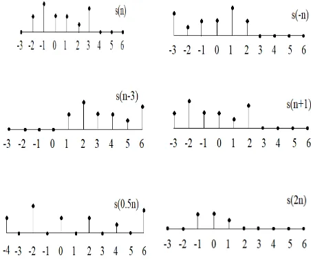
integer value. Also, s(an) dilates s(n) if |a| > 1 and the signal is stretched out, however, if |a| < 1, the signal is compressed. In Fig. 1, a signal s(n) is shown for s(-n), s(n-3), s(n+1), s(0.5n) and s(2n), respectively. The most famous basic sequences in the signal processing are unit sample sequence, which is defined as follows:
0
n
1
0
n
0
)
n
(
(2)
The important aspect of the unit sample sequence (USS) is that an arbitrary signal can be represented as sum of scaled, delayed USS as follows [20]:
k
)
k
n
(
)
k
(
s
)
n
(
s
(3)This concept will be used in filtering the earthquake record.
3.
Discrete signal transformation
A discrete time system is defined as an operator, which
maps an input with values s(n) into an output with
values y(n). One class of this transformation is linear
transformation. The linear system is defined by the
principle of superposition. Another class of system is
time-invariant. A time-invariant system is a system for
which time delays or shift of the input sequence causes
a corresponding shift in the output. If a system
transforms the input s(n) into the output y(n), then the
system is said to be time invariant if, for all n
0the input
S
1(n)=s(n-n
0) produces the output y
1(n)=y(n-n
0).
One of the important classes of systems is linear and
time-invariant systems. These two properties in
combination
lead
to
especially
convenient
representations for such systems. If the linearity
property is combined with the representation of a
general sequence as a linear combination of delayed
impulses, it follows that a linear system can be
completely characterized by its impulse response.
Fig. 1: Examples of s(n) with basic properties
one of the features of time-invariance implies that if h(n) is the response to δ(n) then the response of δ(n-k) is h(n-k), therefore it can be written as:
k
)
k
n
(
h
)
k
(
s
)
n
(
y
(4)As a consequence of Eq. 4, a linear and time-invariant is completely characterized by its impulse response h(n) in the sense that, given h(n), it is possible to use Eq. 4 to compute the output y(n) for any input s(n). Equation 4 commonly is called the convolution sum.
4. Frequency selective filters
A filter can be used to select different frequencies of a signal. A filter is called low-pass if its frequency response is located around zero, and is high-pass if it is around 𝜋. In filters, the frequency response is unity for a certain range of frequencies and is zero for the remaining frequencies. Because of the inherent periodically of the discrete time frequency response, it is similar to a multi band filter, since frequencies around 2𝜋 are indistinguishable from frequencies around 0. The frequency response passes only low frequencies and rejects high frequencies of the signal. Since the frequency response of the signal is completely specified by its behavior over the range
, the ideal low-pass filter frequency response is more typically shown only in range
. It is understood that the frequency response repeats with period of 2𝜋 outside the plotted range.5. Wavelet transform
Wavelet analysis started in the 80’s. Recently, there has been a great interest in wavelet applications in analysis and
Numerical Methods in Civil Engineering, Vol. 2, No. 4, June. 2018 approximation of earthquake [23-24]. The analysis of signals often involves a compromise between how well sudden variations can be located, and how well long-term behavior can be identified. Choosing basis functions well suited for the analysis of signals is an essential step in such applications.
Fourier series are examples of basic functions used in signal approximation. If a signal is piecewise smooth, with isolated discontinuities, the Fourier approximation is poor because of discontinuities. Wavelets are well suited to approximate piece-wise smooth signals. There is an important difference between FT and WT. (sinus and casinos) Fourier basis are localized in frequency but not in time. Wavelets are local in both frequency and time. So, piece-wise smooth signals can be represented by wavelets in a more compact way.
The WT is performed using a single prototype function, ψ. Fine temporal analysis is done by contracted wavelets, whereas fine frequency analysis uses dilated wavelets. The continuous wavelet transform (CWT) of the signal s(n), is named CWT(a,b), and defined as follows [25-26]:
s(n) (n)dn )
b , a (
CWT
a,b (5)) a b n ( a 1 ) n ( b , a
(6)
The wavelets ψa,b(n) are generated from a single basic wavelet ψ(n) that is called mother wavelet by scaling and translation. a is scaling factor, b represents the translation and the factor 1/√𝑎 is for energy normalization across the different scales. Equation 5 shows a signal s is decomposed into a set of basis functions ψa,b(n). For large a, the basis function becomes stretched, while for small a, the basis function becomes a contracted wavelet. The most important properties of wavelets are the admissibility and the regularity conditions and these are the properties that gave wavelets their name [27].
The CWT is highly redundant because (a,b) are continuous. The transformation is usually evaluated by a discrete set of continuous basis functions. For dynamic analysis applications, this redundancy should be removed. Also we have an infinite number of wavelets in the WT and this number must be reduced to a more manageable number. For most functions the wavelet transforms have no analytical solutions and they can be calculated only numerically. To overcome these problems discrete wavelet transform (DWT) have been introduced. This is achieved by modifying the wavelet representation in Eq. 6 by: ) a a kb n ( a 1 ) n ( j 0 j 0 0 j 0 k , j (7)
then DWT of Eq. 5 is:
s(n). (n)dn )
k , j (
DWT j,k
(8)
Where j and k are integers and a0 1is a fixed dilation step.
The factor b0 depends on the dilation step. The effect of
discretizing the wavelet is that the time-scale space is now sampled at discrete intervals. If DWT is used to transform a signal, the result will be a series of wavelet coefficients of signal.
6. Fast wavelet transform
In FWT a scaling function ϕ corresponding to a mother wavelet are used. The scaling function in each level is defined as:
𝜓(2𝑗𝑛) = ∑ ℎ
𝑗+1(𝑘)𝜓(2𝑗+1𝑛 − 𝑘)
𝑘 (9)
where hj+1 is a low-pass filter. The effect of this is that the first scaling function can be expressed in terms of the second one. This is formally called multi resolution formulation or two-scale relation [28]. The two-scale relation states that the scaling function at a certain scale can be expressed in terms of translated scaling functions at the next smaller scale. The scaling function is replaced by a set of wavelets and therefore we can also express the wavelets in this set in terms of translated scaling functions at the next scale. More specifically for the wavelet at level j can be written as:
𝜙(2𝑗𝑛) = ∑ 𝑔
𝑗+1(𝑘)𝜙(2𝑗+1𝑛 − 𝑘)
𝑘 (10)
where gj+1 is a high-pass filter. This equation is the two-scale relation between the scaling function and the wavelet. The signal s could be expressed in terms of translated and dilated wavelets up to a scale j-1, this leads to the result that s can also be expressed in terms of dilated and translated scaling functions at a scale j, as:
k , j j k ,j
(
2
n
k
)
)
k
,
j
(
DWT
)
n
(
s
(11)If in this equation we step up a scale to j-1, we have to add wavelets in order to keep the same level of detail. We can then express the signal s as:
k 1 j 1 j k 1 j 1j (k) (2 n k) (k) (2 n k)
) n (
s (12)
This equation is called inverse wavelet transform (IWT) of the main signal. If the scaling function ϕj,k(n) and the wavelets ψj,k(n) are orthonormal, then the coefficients λj−1(k) and μj−1(k) are found by taking the inner products
as:
1
(
k
)
s
(
n
),
j,k(
n
)
j
(13)
1(k) s(n), j,k(n)
j
(14) By ϕj,k(n) substitution and ψj,k(n) into the inner products and by suitably scaled and translated versions of Eqs. 9 and 10 and manipulating, we obtain an important result [25].
m j 1 j 1j (k) h(m 2k) (m)
AS
(15)) m ( ) k 2 m ( g ) k ( DS j m 1 j 1
j
(16)
23
Equations 15 and 16 state the wavelet and scaling functioncoefficients on a certain scale. From discrete signal processing theory, we know that a discrete weighted sum like the ones in Eqs. 15 and 16 is the same as a digital filter and the coefficients λj(k) come from the low-pass part of the splitted signal spectrum. The weighting factors h(k) in Eq. 15 must form a low-pass filter, and the coefficients μj(k) come from the high-pass part of the splitted signal spectrum. The weighting factors g(k) in Eq. 16 must form a high-pass filter [27]. All the filters used in FWT and IWT are intimately related to the sequence ϕ(n). The filter ϕ, which is called the scaling filter, is a low-pass filter. for filter ϕ, four filters are defined using the following scheme:
) n ( g ) n ( g ) h ( QMF g ) n ( h ) n ( h h R D R R R D R
where QMF is quadrature mirror filter, and defined as: N 2 ,... 2 , 1 k ) k 1 N 2 ( h ) 1 ( ) K ( g R 1 k
R
(17) where h and g are low-pass and high-pass filters, respectively. Subscript D and R are used for decomposition and reconstruction, respectively.
7. The FWT to approximate earthquake record
The FWT decomposition and reconstruction algorithm is used for signals and images. The FWT algorithm is applied for DWT. The FWT permits the computation of the WT. At each level of transform, the signal is processed through a low-pass and a high-pass filter. The high-pass filtered signal is known as the detail wavelet coefficients. The result of the low-pass transform is then decimated by a factor of two and used as input signal at the next level of resolution. After the decimation, the same two filters are applied to the data.
As 𝑆̈shown in Fig. 2, the main earthquake wave has been decomposed using wavelet transform and it's high and low frequencies have been separated. Detailed wave was similar with the main wave but detailed wave is different. The AS̈ approximations wave maintains the frequency content of the main earthquake wave, it is used as new earthquake wave and in next step two new waves are again obtained by this wave. At each stage of the decomposition, the number of generated wave points is half that of the preceding stage wave. In other words, half of the accelerogram points are in detailed wave and the other half in approximation wave. So by halving the number of earthquake points, the time required for dynamic analysis will also decrease with this new wave. Next, the resolution is halved and the frequency resolution is doubled. This idea for calculating discrete wavelet transform, known as the filter bank method, which was carried out in the [6] for the earthquake, and had very good results. Then, using discrete wavelet, approximations wave obtained from the previous stage is decomposed again and two new waves including approximations and detailed waves are obtained. Again it is obtained for approximations
wave. It should be noted that the number of stages required for DWT depends on the frequency characteristics of analyzed signal.
Finally, the DWT of signal is obtained from composition of the outputs of filters in the first stage of filtering.
Fig. 2: Decomposition of record in each level (𝐴𝑆̈0 =𝑆̈ )
A decomposed signal is also reconstructed using a filter bank [24]. This filter bank is an inverse version of the filter bank used for up-sampling. It is used for reconstructing a low-pass filter (h(D)) and high-pass filter (g(D)). It should be noted that these two low-pass and high-pass filters are the same filters used in decomposition. As shown in Fig. 2, the initial signal has a length of one half of the main earthquake signal (N/2), and during two stages of reconstruction (Fig. 3), the length is equal to the main signal (N).
Fig. 3: Reconstruction of record in each level
8. Numerical examples
A SBS is analyzed by El-Centro (S-E 1940) earthquake. Haar wavelet [24] is used for FWT. The Haar wavelet and associated scaling function are as:
otherwise 0 1 x 5 . 0 1 5 . 0 x 0 1 ) n ( (18) otherwise 0 1 x 0 1 ) n ( (19)
A moment magnitude of 6.9 and the number of points of the El-Centro is 2688. It should be noted that this earthquake has not been scaled up. The response of structure is calculated by Newmark method [1]. A personal computer was used and the analyzing time is calculated. The analysis is carried out by following methods:
Numerical Methods in Civil Engineering, Vol. 2, No. 4, June. 2018 (a) Regular dynamic analysis subjected to main
record (DAM)
(b) Dynamic analysis using FFT
(c) Dynamic analysis using FWT and IWT by signals 𝐴𝑆̈1, 𝐴𝑆̈2, 𝐴𝑆̈3and 𝐴𝑆̈4.
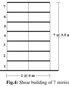
The 7-story SBS model shown in Fig. 4 was analysed, with this assumption that the floor masses move only horizontally. It was assumed that the mass of each rigid floor of the model includes the effect of masses of all the structural elements adjacent to the floor of the prototype building. The mass of each floor is 90 tons. The material properties are given as E=2*106 kg/cm2, weight density of 0.0078 kg/cm3 and damping ratio for all modes of 0.02. Total dimension of the studied frame is 12 and 24.5 m. The bay length is 6 m and story height is 3.5 m.
Fig.4: Shear building of 7 stories
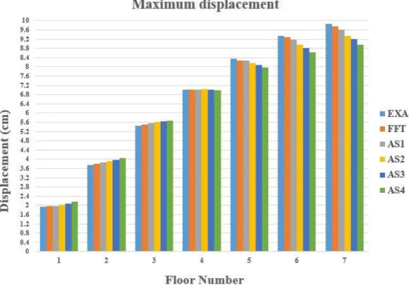
Results of analysis for maximum displacement of each floor for all cases for the El-Centro record are given in Table 1. The displacement history of the top storey, for DAM, and dynamic analysis by 𝐴𝑆̈1, 𝐴𝑆̈2, 𝐴𝑆̈3 and 𝐴𝑆̈4 records are shown in Figs. 5 to 9. The results show that, not only the maximum displacements of each floor are almost the same, but also displacement histories of all the cases are similar. The computation time in DAM is greater than FFT, FFT is greater than 𝐴𝑆̈1, 𝐴𝑆̈1 is greater than 𝐴𝑆̈2is greater than 𝐴𝑆̈3, and 𝐴𝑆̈3 is greater than 𝐴𝑆̈4. The time of analysis for
DAM, FFT, 𝐴𝑆̈1, 𝐴𝑆̈2, 𝐴𝑆̈3 and 𝐴𝑆̈4 are 2.13, 1.31, 0.77, 0.41, 0.21 and 0.11 sec., respectively. The results indicate that as the decomposition process is continued, the time of analysis is reduced but the error involved is increased.
Fig. 5: Displacement history of level 7 using DAM (cm)
Fig. 6: Displacement history of level 7 using 𝐴𝑆̈1 (cm)
Fig. 7: Displacement history of level 7 using𝐴𝑆̈2 (cm)
Fig. 8: Displacement history of level 7 using𝐴𝑆̈3(cm)
Fig. 9: Displacement history of level 7 using𝐴𝑆̈4 (cm)
25
9. Conclusions
Given the numerical results, the following points can be concluded:
(a) The FWT was an effective approach for dynamic analysis.
(b) The overall time required for dynamic analysis was reduced substantially using FWT.
(c) The difference between the exact and approximate analysis was increased as the decomposition was continued.
(d) In each successive decomposition, the time of analysis was reduced by a factor of nearly 2 but the error was increased by a factor of 2.
(e) The best choice for approximation record was the second and third stages of decomposition (𝐴𝑆̈2 and 𝐴𝑆̈3), because, the error of computation is acceptable.
(f) we can separate the low and the high frequency of the record using FWT. The low frequency of record is important, because it contains most of the energy of the record and the shape of the low frequency is similar to the shape of the main record. Therefore, we can analyse the structure against this part. The results are almost similar to those of the original earthquake record. The error is negligible, in particular in the first stages of decomposition.
Table. 1: Results of maximum displacement
Also, the results of Table 1 are shown in figure 10.
Fig. 10: Results of maximum displacement Floor
No.
Maximum dynamic displacement (cm) |EXA-(FFT or 𝐴𝑆̈𝑖)|/EXA*100
EXA FFT 𝐴𝑆̈1 𝐴𝑆̈2 𝐴𝑆̈3 𝐴𝑆̈4 FFT 𝐴𝑆̈1 𝐴𝑆̈2 𝐴𝑆̈3 𝐴𝑆̈4
1 1.950 1.962 1.977 2.036 2.083 2.154 0.6 1.2 4.1 6.3 9.4
2 3.754 3.795 3.857 3.929 3.974 4.057 1.0 2.6 4.3 5.4 7.4
3 5.456 5.510 5.552 5.614 5.633 5.677 0.9 1.7 2.7 3.1 3.8
4 7.025 7.015 7.006 7.046 7.016 6.982 0.2 0.3 0.3 0.1 0.6
5 8.351 8.273 8.271 8.175 8.093 7.968 0.9 1.0 2.2 3.2 4.9
6 9.342 9.299 9.169 8.946 8.831 8.625 0.5 1.9 4.4 5.8 7.3
7 9.873 9.765 9.627 9.335 9.204 8.953 1.1 2.6 5.8 7.3 10.3
Numerical Methods in Civil Engineering, Vol. 2, No. 4, June. 2018
References
[1] Paz, M., Structural dynamics: theory and computation. Springer
Science & Business Media, 2012.
[2] Thambiratnam, D. Zhuge, Y., “Dynamic analysis of beams on
an elastic foundation subjected to moving loads”, Journal of sound and vibration, vol.198, 1996, p.149-169.
[3] Chang TP, Liu YN., “Dynamic finite element analysis of a nonlinear beam subjected to a moving load”, International Journal of Solids and Structures. 1996, vol. 33, p.1673-1688.
[4] Dimitrovová, Z., “A general procedure for the dynamic analysis
of finite and infinite beams on piece-wise homogeneous foundation under moving loads” Journal of Sound and Vibration, vol. 329, 2010, p. 2635-2653.
[5] Salajegheh E. Heidari A. “Dynamic analysis of structures against earthquake by combined wavelet transform and fast Fourier transform”, Asian Journal of Civil Engineering, vol. 3, 2002, p. 75-87.
[6] Salajegheh E. Heidari A. “Time history dynamic analysis of structures using filter banks and wavelet transforms”, Computers and Structures, vol. 83, 2005, p. 53-68.
[7] Heidari A. Salajegheh E. “Time history analysis of structures
for earthquake loading by wavelet networks”, Asian Journal of Civil Engineering, vol. 7, 2006, p. 155-168.
[8] Heidari A. Salajegheh E. “Approximate dynamic analysis of
structures for earthquake loading using FWT”, International Journal of Engineering (IJE), I.R.I., vol. 20, 2007, p. 37-47.
[9] Kaveh A. Aghakouchak AA. Zakian P. “Reduced record
method for efficient time history dynamic analysis and optimal design. Earthquakes and Structures”, vol. 8, 2015, P. 639-63.
[10] Naseralavi SS. Balaghi S. Khojastehfar E. “Effects of Various
Wavelet Transforms in Dynamic Analysis of Structures”. World Academy of Science, Engineering and Technology, International Journal of Civil, Environmental, Structural, Construction and Architectural Engineering. Vol. 10, 2016, p. 860-4.
[11] Salajegheh E. Heidari A. “Optimum design of structures against earthquake by adaptive genetic algorithm using wavelet networks”, Structural and Multidisciplinary Optimization, vol. 28, 2004, p. 277-285.
[12] Salajegheh E. Heidari A. “Optimum design of structures
against earthquake by wavelet transforms and filter banks”, International Journal of Earthquake Engineering and Structural Dynamics, vol. 34, 2004, p. 67-82.
[13] Salajegheh E. Heidari A. Saryazdi S. “Optimum design of structures against earthquake by discrete wavelet transform,” International Journal for Numerical Methods in Engineering, vol. 62, 2005, p. 2178-2192.
[14] Heidari A. “Optimum design of structures for earthquake induced loading by genetic algorithm using wavelet transform”, Advances in Applied Mathematics and Mechanics, vol. 2, 2010, p. 107-117.
[15] Gholizadeh, S., Samavati, O.A., “Structural optimization by wavelet transforms and neural networks”, Applied Mathematical Modelling, vol. 35, 2011, p. 915-29.
[16] Heidari, A., Raeisi, J. "Optimum Design of Structures Against earthquake by Simulated Annealing Using Wavelet Transform". Soft Computing in Civil Engineering, vol. 2, 2018, p. 23-33.
[17] Polikar R. “The Wavelet Tutorial”,
http://www.public.iastate.edu/~rpolikar/WAVELETS/ wave
letindex html, 1996.
[18] Chen, W.K., The circuits and filters handbook. CRC Press, Inc, 2009.
[19] Strang G., Nguyen T. “Wavelets and Filter Banks”, New York:
Wellesley-Cambridge Press, 1996.
[20] Roerdink J.B.T.M. “Wavelets for Signal and Image
Processing”, Lecture notes, Department of Computing Science, Rijksuniversiteit Groningen, NL, 1993.
[21] Kaveh, A., Mahdavi, V. R., “A new method for modification of ground motions using wavelet transform and enhanced colliding bodies optimization”, Applied Soft Computing, vol. 47, 2016, p. 357-369.
[22] Heidari, A., Raeisi, J., Kamgar, R., “Application of wavelet
theory in determining of strong ground motion
parameters”, Internarial. Journal of Optimization in Civil Engineering, vol. 8, 2018, p. 103-115.
[23] Wang, Z., Zhang, B., Gao, J., Wang, Q., Huo Liu, Q., Wavelet transform with generalized beta wavelets for seismic time-frequency analysis. Geophysics, vol. 82, 2017, pp.O47-O56.
[24] Pnevmatikos, N.G., Hatzigeorgiou, G.D., Damage detection
of framed structures subjected to earthquake excitation using discrete wavelet analysis. Bulletin of Earthquake Engineering, vol. 15, 2017, pp.227-248.
[25] Oppenheim A.V., Schafer R.W., Buck J.R. “Discrete-Time
Signal Processing”, New Jersey: Prentice Hall, 1999.
[26] Thuillard M. “Wavelets in Soft Computing”, New York:
World Scientific Publishing Co. Pte. Ltd., 2001.
[27] Burrus C.S., Gopinath, R.A., Guo. H. “Introduction to
Wavelets and Wavelet Transforms, a Primer”, New Jersey: Prentice Hall, 1998