R E S E A R C H A R T I C L E
Open Access
Bayesian structured additive regression modeling
of epidemic data: application to cholera
Frank B Osei
1*, Alfred A Duker
2and Alfred Stein
3Abstract
Background:A significant interest in spatial epidemiology lies in identifying associated risk factors which enhances the risk of infection. Most studies, however, make no, or limited use of the spatial structure of the data, as well as possible nonlinear effects of the risk factors.
Methods:We develop a Bayesian Structured Additive Regression model for cholera epidemic data. Model estimation and inference is based on fully Bayesian approach via Markov Chain Monte Carlo (MCMC) simulations. The model is applied to cholera epidemic data in the Kumasi Metropolis, Ghana. Proximity to refuse dumps, density of refuse dumps, and proximity to potential cholera reservoirs were modeled as continuous functions; presence of slum settlers and population density were modeled as fixed effects, whereas spatial references to the communities were modeled as structured and unstructured spatial effects.
Results:We observe that the risk of cholera is associated with slum settlements and high population density. The risk of cholera is equal and lower for communities with fewer refuse dumps, but variable and higher for
communities with more refuse dumps. The risk is also lower for communities distant from refuse dumps and potential cholera reservoirs. The results also indicate distinct spatial variation in the risk of cholera infection.
Conclusion:The study highlights the usefulness of Bayesian semi-parametric regression model analyzing public health data. These findings could serve as novel information to help health planners and policy makers in making effective decisions to control or prevent cholera epidemics.
Keywords:Bayesian, Cholera, Cholera reservoir, Refuse dumps, Slums
Background
A significant interest in understanding the epidemiology of diseases lies in identifying associated risk factors which enhance the risk of infection, the so called eco-logical studies [1,2]. Most of these ecological studies, however, make no, or limited use of the spatial structure of the data, neither do they consider possible nonlinear effects of the risk factors. Thus, most studies use stand-ard statistical methods such as the classical and general-ized linear models that ignore methodological difficulties that arise from the nature of the data. Ali et al. [3,4] have used logistic, simple and multiple linear regression models to study the spatial epidemiology of cholera in an endemic area of Bangladesh. Other ecological studies of cholera that have utilized standard statistical methods
include Ackers et al. [5], Mugoya et al. [6] and Sasaki et al. [7]. These methods when applied to spatially dis-tributed data present severe problems with estimating small area spatial effects, and simultaneously adjusting for other risk factors, in particular if such effects are nonlinear. If standard statistical methods are used to analyze spatially correlated data, the standard error of the covariate parameters is underestimated and thus the statistical significance is overestimated [8].
Generalized additive models (GAM) provide a power-ful class of models for modeling nonlinear effects of continuous covariates in regression models with non-Gaussian responses. Structured Additive Regression (STAR) models are extensions of GAM models that allow one to incorporate small area spatial effects, non-linear effects of risk factors, and the usual non-linear or fixed effects in a joint model [9]. This study applies a STAR * Correspondence:[email protected]
1
Faculty of Public Health and Allied Sciences, Catholic University College of Ghana, Sunyani/Fiapre, Ghana
Full list of author information is available at the end of the article
modeling approach to develop a multivariate explanatory model for cholera.
Cholera outbreak is enhanced by several environmen-tal and/or socioeconomic risk factors once introduced in a population. Ali et al.[3,4] identified proximity to sur-face water, high population density, and low educational status as the important risk factors of cholera in an en-demic area of Bangladesh. Borroto and Martinez-Piedra [10] identified poverty, low urbanization, and proximity to coastal areas as the important geographic risk factors of cholera in Mexico. Sanitation is an important envir-onmental risk factor that predisposes inhabitants to cholera infection. Previous ecological studies have used spatial regression models to explore the dependency of cholera on some local measures of sanitation [11,12]. No attempt, however, has been made to combine all the identified measures of sanitation, including spatial effects, into a single multivariate model to examine their joint effects on cholera. In this study, we exploit the joint effects of three main spatial measures of sanitation identified from previous studies [11,12]. These are dens-ity of refuse dumps, proximdens-ity to refuse dumps and proximity to potential cholera reservoirs. Other risk fac-tors used in this study include livelihood at slummy and squatter environments [13], and population density [3,4,14,15]. Livelihood at slummy and squatter environ-ments increase the risk of cholera infection, whereas high population density stresses existing sanitation sys-tems, thus putting people at increased risk of cholera.
This study incorporates the effects of nonlinear risk factors and the usual fixed effects of some risk factors, while accounting for both structured and non structured
spatial effects. A STAR model of this type has been termed geoadditive model [16,17]. The increasing avail-ability of disease and environmental data necessitate the development of such models to obtain valid and realistic statistical inferences that adequately describe the vari-ation of the disease. Proximity to dumps, density of dumps, and proximity to potential cholera reservoirs are modeled as smooth continuous functions, whereas pres-ence of slum settlers and population density are modeled as fixed effects, and spatial references to the communi-ties are modeled as structured and unstructured spatial effects. We use a fully Bayesian estimation based on Markov Chain Monte Carlo (MCMC) simulations using simple Gibbs sampling updates. Making inferences based on a fully Bayesian approach is preferred because the functionals of the posterior can be computed without relying on large Gaussian justifications, thereby quantify-ing the uncertainty in the parameters [18].
Methods
Study area and cholera data
This study is based on the 2005 cholera outbreak in Kumasi Metropolis, Ghana. Kumasi Metropolis is com-pletely urban and the most populous city in Ashanti Region. It is located at the intersection of latitude 6.04°N and longitude 1.28°W, covering an area of approximately 220 km2(See Figure 1). Kumasi has a population of ap-proximately 1.2 million. Surveillance and reporting of the disease before 2005 has been ineffective, and hence the existing data before 2005 have little or no spatial in-formation. However, with intensified surveillance and reporting systems during an outbreak in 2005, disease
cases in Kumasi are available at community level spatial units. This makes the Kumasi area suitable for such a study. During the outbreak in 2005, cholera incidence rates ranged from 0.47 to 31.92 per 10,000 people (mean= 10.21,standard deviation= 6.84).
The topographic map of the metropolis and then = 68 communities where cholera records are available was digitized. Cholera data for each community was extracted from disease records of the Kumasi Metropol-itan Disease Control Unit (DCU). We accessed such data based on special permissions given by the Kumasi DCU. The centroids of the communities were used as the spatial references of cholera cases since residential addresses were not recorded during the outbreak. The denominator (population data) for computing community-specific cholera rates was obtained from the 2000 Popu-lation and Housing Census of Ghana [19].
Model specification
For each communityi, i¼1;. . .;N of populationPi, the
observed number of cholera casesCholð ÞOi is assumed to
be a realization of random variable that follows indepen-dent Poisson distribution with intensityCholð ÞEiCholð ÞRi;
thus:Cholð ÞOi Cholð ÞRiPoisson Cholð ÞEiCholð ÞRi
, where
Cholð ÞEi is the expected number of cholera cases and
Cholð ÞRiis the relative risk of cholera infection. A
com-mon practice is to estimateCholð ÞEi asCholð ÞR Pi, where
Cholð ÞR is the overall risk of cholera infection within the
study population obtained as a weighted average of the community-specific rates, each weighted by their share in the overall population; thus:
CholðRÞ¼
XN i¼1
Cholð ÞOi
Pi
Pi
PN i¼1Pi
:
For ease of interpretation, we use the relative risk (also called excess risk) as the reference benchmark to esti-mate the risk of cholera infection. We consider the triple ðCholðRÞi;xi;wiÞ;i¼1;. . .;N where Cholð ÞRi is the
rela-tive risk of cholera infection in communityi. The vector xi¼ ðxi1;. . .;xipÞ′ contains the p continuous covariates
and wi¼ ðwi1;. . .;wirÞ′ is a vector ofrcategorical
cov-ariates. In our study, p =3 and r =2.The study assumes that the response variable Chol(R) is Gaussian distribu-ted, i.e.Cholð ÞRiηi;σ2eNðηi;σ2Þ, with an unknown mean
ηiwhich can be expressed in the form:
ηi¼x′iβþw′iγ: ð1Þ
Here, βis ap-dimensional vector of unknown regres-sion coefficients for the continuous covariates xi, and γ
is a r-dimensional vector of unknown regression coeffi-cients for the categorical covariateswi.
In order to account for both the nonlinear effects of the continuous covariates and the spatial dependence of the data, a geoadditive modeling approach is re-quired [16]. The geoadditivemodel replaces the strictly linear predictor by a more flexible semi-parametric predictor as:
ηi¼f1 xi;1 þ. . .þfp xi;p þfspatð Þ þsi w′iγ: ð2Þ
Here, f1ð Þx ;. . .;fpð Þx are nonlinear smooth functions
of the continuous covariates xi;1;. . .;xi;p and fspatð Þsi is a
function that accounts for spatial effects at each commu-nity si2f1;. . .;Sg. Spatial effect is usually a surrogate
of unobserved influential factors, some of which may have a strong spatial structure and others may be present only locally (unstructured). To distinguishing be-tween the two kinds of influential factorsfspatð Þs is split
up into spatially correlated (smooth) part fstrð Þs and
spatially uncorrelated (unsmooth) part funstrð Þs , i.e.
fspatð Þ ¼s fstrð Þ þs funstrð Þs .
The finalgeoadditivemodel is then expressed as:
ηi¼f1 xi;1 þ. . .þfp xi;p þfstrð Þ þsi funstrð Þsi
þw′iγ:
ð3Þ This model contains p+ 2 functions and rfixed para-meters to be estimated.
Prior distributions for covariates
A fully Bayesian approach for modeling and inferences requires prior assumptions for the unknown functions fjð Þx ;funstrð Þs;fstrð Þs and the fixed effect regression
par-ameterγ. Forγ, we assume an independent diffuse prior pð Þ /γ constdue to the absence of any prior knowledge. A possible alternative choice is a weak informative multivariate Gaussian distribution.
For the continuous functions fjð Þx;j¼1;. . .;p, we
choose the Bayesian P(enalized)-splines [20,21]. This ap-proach assumes that an unknown smooth functionfj of
a covariate xj can be approximated by a polynomial
spline of degree l defined on a set of equally spaced knots xmin
j ¼ζj;0<ζj;1<⋯<ζj;s1<ζj;s¼xmaxj within
the domain ofxj. Such a spline can be written in terms
of a linear combination of d¼sþl basis functions Bm, i.e.
fj xj ¼
Xd m¼1
ξj;mBm xj : ð4Þ
The B-splines form a local basis since the functions Bm are only positive within an area spanned by l+ 2
unknown regression coefficients ξj¼ ðξj;1;. . .;ξj;mÞ′
from the data. An essential factor in the estimation pro-cedure is the choice of the number of knots. We chose a moderately large number of equally spaced knots (20), as suggested by Eilers and Marx [20] to ensure enough flexibility to capture the variability of the data. In the Bayesian approach, penalized splines are introduced by replacing the difference penalties with their stochastic analogues, i.e., first or second order random walk priors for the regression coefficients. A first order random walk prior for equidistant knots is given by:
ξj;m ¼ξj;m1þuj;m;m¼2;. . .;d; ð5Þ
and a second order random walk for equidistant knots by:
ξj;m ¼2ξj;m1ξj;m2þuj;m;m¼3;. . .;d; ð6Þ
where uj;meN 0;τ2j
are Gaussian errors. Diffuse priors
ξj;1/const, or ξj;1 andξj;2/const, are chosen as initial values, respectively. The joint distribution of the regres-sion parametersξj;mfor a first order random walk is
defined as:
ξj;m ξj;m1eN ξj;m1;τ2j
;
ð7Þ
and a second order random walk is defined as:
ξj;m ξj;m1;ξj;m2eN 2ξj;m1ξj;m2;τ2j
:
ð8Þ
The first order random walk induces a constant trend for the conditional expectation of ξj;m given ξj;m1and a second order random walk results in linear trend de-pending on the two previous values ξj;m1and ξj;m2. The joint distribution of the regression parameters ξj¼
ξj;1;. . .;ξj;m
′
is computed as a product of the condi-tional densities defined by the random walk priors. The general form of the prior forξjis a multivariate Gaussian
distribution with density:
p ξjjτ2j
/ exp ξ
′
jKjξj
2τ2
j
!
; ð9Þ
where the precision matrix Kj acts as a penalty matrix
that shrinks parameters towards zero, or penalizes too abrupt jumps between neighboring parameters. Since the penalty matrix Kj is rank deficient, i.e.kj¼rank Kj <
dim ξj ¼dj, it follows that the prior forξjτ2j is partially
improper with Gaussian priorξjτ2j /N 0;τ2jKj
, where
Kjis a generalized inverse of Kj. The tradeoff between
flexibility and smoothness is controlled by the variance
parameter τ2j. A large variance corresponds with a rough estimated function, and vice versa.
Spatial components
We use the nearest neighbor Gaussian Markov random field model which is common in spatial statistics to ex-press prior knowledge of the structured spatial effects. Suppose s2f1;. . .;Sgrepresent the locations of con-nected communities, then the locally dependent prior probability spatial structure can be specified as:
fstrð Þs fstr s′ ;s′6¼s;τ2streN
1 Ns
X
s′2@s
fstr s′ ;τ
2 str Ns ! ;
ð10Þ
where Ns is the number of adjacent spatial units and
s′2@sdenotes that spatial units’is a neighbor of spatial unit s. Thus, the conditional mean of fstr (s) is an
unweighted average of the function evaluations of neigh-boring spatial units. Since only the centroids of commu-nities (point data) are available, we assume the effect of spatial interaction is dependent on distance between the centroids of pair of communities. To ensure equal num-ber of neighbors for each community we chose a neigh-borhood structure based on the kth nearest neighbor method (where k is the number of neighbors). This ap-proach results in an asymmetric neighborhood matrix; therefore, false symmetry was imposed to ensure a sym-metrical neighborhood structure. Like the continuous functionsfj, the tradeoff between flexibility and
smooth-ness is controlled by the variance parameterτ2
str.
For the unstructured spatial effects, we assume that the parametersfunstr(s) arei.i.d. Gaussian:
funstrð Þs τ2unstr N 0;τ2unstr
:
ð11Þ
Hyperpriors for the variance or smoothness para-meters τ2
j;j¼1;. . .;p;str, unstr, are considered as
un-known. Therefore, highly dispersed, but proper, inverse
Gamma distributions p τ2
j IG aj;bj
with known
hyper-parameters αj and bj are assigned in the second
stage of the hierarchy. The corresponding probability density function is expressed as:
p τ2j / τ2j aj1exp bj
τ2
j
!
: ð12Þ
Bayesian inference
Bayesian inference stems from the posterior distribution, that is, the conditional distribution of the model para-meters given the observed datapθCholð ÞR, where θ
denotes the vector of all model parameters, Chol(R) the data vector,p(.) represents the probability density func-tion. In this study, we use a fully Bayesian inference based on analysis of posterior distribution of the model parameters by drawing random samples via MCMC simulation techniques. The probability density function of the posterior distribution is expressed as:
where L (.) is the likelihood function. The full condi-tional for the variance components τ2j;j¼1;. . .;p;str, unstr, andσ2 are inverse Gamma distributions. The full conditional for the fixed parametersγ, the unknown par-ameter vectorξ1;. . .;ξp, as well as fstrð Þs ;funstrð Þs are
multivariate Gaussian. Gibbs sampler was employed for MCMC simulations, drawing successively from the full conditionals for the variance components and the un-known parameters. Cholesky decompositions for band matrices were used to efficiently draw random samples from the full conditional [22,23].
Model implementation
The continuous covariates used in this study are proxim-ity to refuse dumps ddumps,density of refuse dumpsρdump,
andproximity to potential cholera reservoirs dreser. These
variables are extracted on per community basis via a Geographic Information System (GIS). Details of the approaches for the calculation of these variables can be found in Osei and Duker [11] and Osei et al.[12]. The spatial locations of the communities are used to model the spatial effects. In the Kumasi area no administrative boundaries are present separating the communities. For ease of visualization and interpretation, the centroids of the communities are converted to Thiessen polygons whose boundaries define the area that is closest to each centroid relative to all other centroids.
In addition, two binary categorical covariates are used; presence of slum settlers in a community ςslumand
popu-lation density ρpop. For communities within which slum
settlers dwell, ςslum =1, otherwise ςslum=0. Since the
boundaries of the various communities do not exist the population density could not be quantified as continuous variable. Therefore, we categorized the population dens-ity as moderately populated ρpop¼0 and densely popu-latedρpop¼1. We analyze the following set of models.
Model1:ηi ¼ρ′
dumpβ1þd′dumpβ2þd′reserβ3þρ′popγ1 þς′
slumγ2 Model2:ηi
¼f1 ρdump
þf2 ddump
þf3ðdreserÞ
þρ′
popγ1þς′slumγ2 Model3:ηi
¼f1 ρdump
þf2 ddump
þf3ðdreserÞ þfstrð Þs
þfunstrð Þ þs ρ′popγ1þς′slumγ2
Model 1 is a strictly linear regression that assumes a linear effect of the categorical and continuous covariates. Model 2 is an additive model which assumes nonlinear functions for the continuous covariates and linear effects of the categorical covariates. Model 3 is a geoadditive model, which is an extension of Model 2 that incorpo-rates both structured and unstructured spatial effects.
The models were implemented in the public domain software BayesX ver 2.0 [24,25]. We used a total number of 40,000 MCMC iterations and 10,000 number of burn in samples. Since, in general, these random numbers are correlated, only every 20th sampled parameter of the Markov chain were stored. This yielded 2,000 samples for parameter estimation. Convergence checks of the MCMC algorithms were based on autocorrelations and the sampling paths.
We compared the strictly linear models with the addi-tive models and the geoaddiaddi-tive models using the Devi-ance Information Criterion (DIC) values [26]. DIC is a Bayesian tool for model checking and comparison, where the model with the smallestDICis preferred. The DICis given byDIC¼DþpD, where D is the posterior
mean of the deviance, which is a measure of goodness of fit, and pD is the effective number of parameters, which
is a measure of model complexity and penalizes over-fitting.
Results
Model selection
Model assessment and selection was based on the com-puted values for the goodness of fit (see Table 1). Models with a smaller DIC value are preferred. Again, models with differences in DIC of less than 3 cannot be pðθjCholÞ /Y
n i¼1
L
CholðRÞi;ηi
Y
p j¼1
½
pðξjjτ2jÞpðτ2jÞpðfstrjτ2strÞpðfunstrjτ2unstrÞYr j¼1
distinguished, while those between 3 and 7 can be weak-ly differentiated [27]. Comparing goodness of fit of models, Model 3 is the preferred model. Although the extension of the basic model (Model1) to an additive model (Model 2) is an improvement; this improvement is indistinguishable (DIC= 43.25 in Model 1 versusDIC= 41.30 in Model 2, IC¼1:95). The extension of Model 2 to include structured and unstructured spatial effects in Model3 significantly improved the model (DIC= 20.07 in Model 3 versus DIC= 41.30 in Model 2, IC¼21:23 ). Therefore, subsequent analysis and discussions are based on the results of Model 3.
Fixed and nonlinear effects of covariates
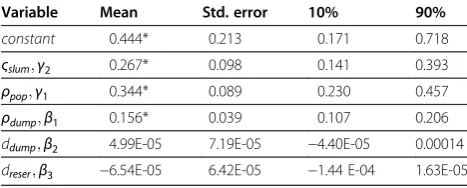
The purpose of Model 1 has been to investigate the ap-propriateness of including nonlinear effects in disease modeling. In Model 1, the continuous covariates ρdump
and dreser are observed to have no significant effect on
Chol(R)which would have led to an erroneous rejection of the significance of their effect (Table 2). In Model 3, the effects of the categorical covariates are assumed fixed are estimated jointly with the continuous and spatial covariates. The posterior means and the corre-sponding 90% credible intervals of the fixed effect para-meters are shown in Table 3. The risk of cholera infection is observed to be associated with high popula-tion density and livelihood at slummy environments. Moderate difference occurs between the risk of infection in populous communities and the risk of infection in slummy. Thus the effect ofρpoponChol(R)is 0.32 (0.20 -0.44) and the effect of ςslum on Chol(R) is 0.28 (0.16 -0.40). The nonlinear effects of ρdump, ddump, and dreser
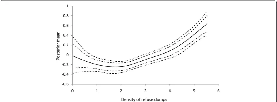
are shown in Figures 2, 3, and 4, respectively. The rela-tionship betweenChol(R)andρdumpis nonlinear, with an
expected increasing risk (Figure 2), preceded by approxi-mate equal risk up toρdump¼1:8 . In other words, the risk of cholera infection is equal and lower for commu-nities with fewer refuse dumps, but increases with in-creasing refuse dumps fromρdump¼1:8 . For ddump, the
risk of infection remains constant up to approximately 500 m, and then deviates from linearity with a general decreasing trend (Figure 3). The effect ofdreser is almost
linear, with the posterior mean decreasing with increas-ing distance (Figure 4).
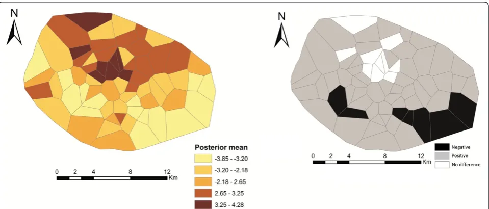
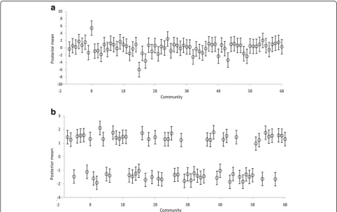
Spatial effects
Figure 5 shows the estimated total spatial effects (left) and the corresponding 80% (credible interval) posterior probability map (right) of cholera risk. Areas shaded black show strictly negative credible intervals, while white areas depict strictly positive credible intervals, and grey indicate areas of non-significant spatial effects. There is evidence of significant clustering of cholera, with higher cholera risk occurring at the central part, and a lower risk occurring at the south-eastern part (the periphery) of Kumasi (Figure 5). The unstructured spatial effects are dominant over the structured spatial effects. This is shown by the higher ratio of variance componentsϕunstr ¼τ2
unstr= τ2strþτ2unstr
¼0:64 (Table4). The lesser variations in the caterpillar plots of Figure 6a compared with Figure 6b also confirms that the unstruc-tured spatial effects are dominant over the strucunstruc-tured spatial effects.
Sensitivity analyses
Since the regression parameters depend on the choice of hyper-parameters, we rerun the MCMC simulations, using Model 3 for simplicity, to investigate the sensitivity of our results to different choices of hyper-parameters. In particular, the following alternatives of priors have been investigated: IG (a= 0.01, b= 0.01), IG (a= 0.5, b= 0.0005) andIG(a= 1,b= 0.005). The first alternative and the standard option IG (a= 0.001, b= 0.001) are commonly used choices for the variances of random effects. The second and third alternatives are suggested by Kelsall and Wakefield [28] and Besag and Kooperberg Table 2 Estimates of fixed effect parameters based on the
linear Model 1
Variable Mean Std. error 10% 90%
constant 0.444* 0.213 0.171 0.718
ςslum;γ2 0.267* 0.098 0.141 0.393
ρpop;γ1 0.344* 0.089 0.230 0.457
ρdump;β1 0.156* 0.039 0.107 0.206
ddump;β2 4.99E-05 7.19E-05 −4.40E-05 0.00014
dreser;β3 −6.54E-05 6.42E-05 −1.44 E-04 1.63E-05
* Significance atp <0 .01.
Table 3 Estimates of posterior mean and 90% credible intervals for the fixed effects for Model 3
Variable Mean Std. error 10% 90%
Constant 0.73* 0.081 0.63 0.83
ςslum;γ2 0.28* 0.095 0.16 0.40
ρpop;γ1 0.32* 0.092 0.20 0.44
*Significance atp <0 .01. Table 1 Comparison of model fit using Deviance
Information Criterion (DIC)
Model Fit Model 1 Model 2 Model 3
D 37.40 32.35 10.64
pD 5.85 8.95 9.43
DIC 43.25 41.30 20.07
ΔDIC
} 23.18 21.23 Reference
[27], respectively. Results of the sensitivity analysis on the choice of hyper-parameters α and b are shown in Table 4. It is noticed that the four choices of hyper-parameters yielded similar inferences for the posterior means of the fixed parameters. Minor differences, how-ever, occur between the variance parameters for the nonlinear functions and the spatial effects suggesting the robustness of our choices. Thus, indicating that our model is less sensitive to the choice of hyper-parameters.
Discussion
This study utilizesgeoadditivemodeling approach to de-velop a multivariate explanatory model for the risk of cholera. We utilize a Bayesian semi-parametric regres-sion model to elucidate the probability of cholera infec-tion in relainfec-tion to associated risk factors, some identified
from previous studies [11,12]. Thegeoadditivemodeling approach is an extension of the GAM which allows the inclusion of both structured and unstructured spatial effects to account for possible unobserved factors and heterogeneity terms. To allow flexibility, the continuous covariates are modeled non-parametrically as nonlinear functions using P-splines with second-order random walk priors based, this based on contributions by Farhmeir and Lang [29,30] and Fahrmeir et al. [18]; while the categorical covariates are modeled as fixed effects. The spatially structured and unstructured effects are modeled using Markov random filed priors and zero mean Gaussian heterogeneity priors, respectively [31]. In this modeling approach, fully Bayesian inferences based on MCMC simulations are preferred because the func-tionals of the posterior can be easily computed, thereby Figure 2The estimated nonlinear effects of cholera risk on of proximity to refuse dumps in Kumasi.The posterior mean together with the 80% and 90% credible intervals are shown.
easily quantifying the uncertainty in the estimated para-meters [18].
The findings of the study show that the risk of cholera infection is high amongst inhabitants dwelling in slums. The risk of infection is also relatively high in densely populated communities. These relationships may exist because most communities with slummy settlers are densely populated. Although cholera is transmitted main-ly through contaminated water or food, poor sanitary conditions in the environment enhance its transmission. The choleravibrioscan survive and multiply outside the human body and can spread rapidly where living condi-tions are overcrowded and where there is no safe disposal
of solid waste, liquid waste, and human feces [3,4]. These conditions are mostly met in slummy and densely popu-lated communities in Kumasi. Such high population density may necessarily result in shorter disease trans-mission paths, thus increasing the risk of cholera in-fection. Also, inhabitants living at slummy areas are generally poor, and face problems including access to potable water and sanitation. In many cases public util-ities providers (e.g. water distribution) legally fail to serve these urban poor due to factors regarding land tenure system, technical and service regulations, and city devel-opment plans. Most slum settlements are also located at low lying areas susceptible to flooding. Unfavorable Figure 4The estimated nonlinear effects of cholera risk on proximity to potential cholera reservoirs in Kumasi.The posterior mean together with the 80% and 90% credible intervals are shown.
topography, soil, and hydro-geological conditions make it difficult to achieve and maintain high sanitation stan-dards among such inhabitants [10].
The risk of cholera infection is observed to decrease with increasing distance from refuse dumps, inhabitants within 500 m away from the refuse dumps being the
most vulnerable. This is consistent with the finding from previous studies when a quantitative assessment of crit-ical distance discrimination on experimental buffer zones around refuse dumps showed that the optimum spatial discrimination of cholera occurs at 500 m way from refuse dumps [11]. Therefore, we hypothesize that Table 4 Summary of the sensitivity analysis of the choice of hyper-parameters for Model 3
a= 0.001 a= 0.01 a= 0.5 a= 1
b= 0.001 b= 0.01 b= 0.0005 b= 0.005
Spatial effects{
fstrð Þs,τ2str 0.02 0.028 0.004 0.004
(0.0005 - 0.0.06) (0.003 - 0.07) (0.00009 - 0.01) (0.0006 - 0.0009)
funstrð Þs,τ2unstr 0.02 0.031 0.007 0.0071
(0.0009 - 0.0.057) (0.005 - 0.056) (0.0001 - 0.028) (0.0006 - 0.019)
Smooth functions}
f1 ρdump
,τ2
1 0.003 0.006 0.0014 0.002
(0.0005 - 0.006) (0.002 - 0.013) (0.0002 - 0.003) (0.0006 - 0.004)
f2 ddump
,τ2
2 0.003 0.0078 0.0007 0.002
(0.0002 - 0.0058) (0.002 - 0.017) (0.00008 - 0.0015) (0.0004 - 0.004)
0.001 0.004 0.0004 0.001
f3ðdreserÞ,τ23 (0.0002 - 0.0024) (0.001 - 0.009) (0.00006 - 0.0007) (0.0004 - 0.003)
{Variance components and 90% credible intervals for the spatially structured and unstructured effects;}variance components and 90% credible intervals for the nonlinear smooth functions.
refuse dumps located within 500 m away from inhabi-tants enhance the risk of cholera infection compared with those farther. The expected decreasing trend of Chol(R)fromddump≥500 m, however, is apparently grounds
for strengthening the acceptance of this hypothesis. Collectively, the nonlinear effects of ddump and ρdump
on Chol(R) suggest that cholera risk is relatively high amongst inhabitants who live in close proximity to re-fuse dumps, and where there are numerous rere-fuse dumps. Due to the bad defecation practices of most inhabitants, the refuse dumps may contain high fecal matter. Surface drainage from such refuse dumps pol-lutes water sources with feces which when used per-petuates the transmission of cholera vibrios. If the runoff from waste dumps during heavy rains serve as the major pathway for fecal and bacterial contamin-ation of rivers and streams, then it is likely that inha-bitants living closer to water bodies where these runoffs flow into will have higher cholera prevalence than those who live farther. The observed decreasing cholera prev-alence with increasing distance from potentially polluted surface water bodies (Figure 4), and the significant linear relationship between ddump and dreser (results
from preliminary regression analysis: β=0.67, R2=0.34, p <0.001) support this hypothesis.
Cholera is primarily driven by environmental and socio-economic factors [3,4]; prior knowledge indicates that geo-graphically close communities will tend to have similar relative risks. Thus, indicating the existence of structured spatial variation in the relative risk. The structured spatial effects included in the model are surrogate measures of unobserved spatially correlated risk factors of cholera. The results show clear evidence of significant clustering of cholera, with higher cholera risk occurring at the central part (the Central Business District), and a lower risk oc-curring at the south-eastern part (the periphery) of Kumasi (Figure 5). These patterns clearly indicate possible unobserved risk factors of cholera, which may be global or local. For example, the increased risk at the central part of Kumasi may be an influence of high daily influx of traders and civil workers from other communities to the Central Business District. Such a high daily influx strain existing sanitation systems which consequently put people at increased risk of cholera. The dominancy of the unstruc-tured spatial effects over the strucunstruc-tured spatial effects indi-cates that the unobserved risk factors are more local than global. For instance, household socioeconomic character-istics may cause such local spatial variation. Therefore, this gives leads for further epidemiological research using add-itional information at household spatial scale within the study area.
Unlike classical modeling approaches, our methodo-logical concept allows modeling flexibility which can re-veal salient features of the continuous covariates. For
instance, the utilization of only the linear model, Model 1, would have led to an invalid rejection of the signifi-cance of some important risk factors: density of refuse dumps, and proximity to potential cholera reservoirs. Such modeling approach is useful to establish a better epidemiological relationship that exists between the dis-ease and the risk factors. Although the methodological concept is somewhat mathematically intensive, the avail-ability of the public domain software, BayesX, provides opportunities for nonprogrammers to utilize these methods.
Limitations of study
Data limitations have enforced this study to be under-taken within a single-scale framework; therefore, signifi-cance of scale effects has not been accounted for in this study. Consequently, possible biases induced by modifi-able areal unit problem (MAUP) have been ignored. If data at different levels of spatial scales were available, possible bias of MAUP would be evaluated within a multi-scale analysis framework as exemplified in Odoi et al. [32]. Moreover, re-aggregating the data to another set of areal units could assess the possible bias of MAUP [33]. However, this is impossible due to the limited avail-ability of higher resolution data and difficulties in asses-sing the ecological fallacy associated. In accordance with the general rule of practice, the study analyzed aggre-gated data using the smallest areal units for which data were available to ameliorate the effects of aggregation. Accordingly, statistical inferences in this study are em-phasized on the group-level rather than the individual-level.
Also, our choice of neighborhood structure induces an assumption that all the inhabitants reside at the centroid of the communities. In reality, the communities have boundaries whereby their adjacency reflects the true na-ture of the spatial strucna-ture. Also, the maps of the spatial effects should be interpreted with caution as the spatial boundaries used are artificial (Thiessen polygons). Per-haps different spatial patterns may be visually observed if the true boundaries of the spatial units existed.
Conclusion
distinct spatial patterns exhibited by the spatial covari-ates; suggesting the need for further epidemiological re-search. These findings should serve as novel information to help health planners and policy makers in making ef-fective decisions about cholera control measures.
Competing interests
The authors declare that they have no competing interests.
Authors’contributions
FBO carried out the research and drafted the manuscript. AAD and AS guided the research and reviewed the manuscript. All authors read and approved the final manuscript.
Acknowledgements
We extend our sincere appreciation to the Kumasi Metropolitan Health Directorate for providing all the necessary data and background information for this research.
Author details 1
Faculty of Public Health and Allied Sciences, Catholic University College of Ghana, Sunyani/Fiapre, Ghana.2Department of Geomatic Engineering,
Kwame Nkrumah University of Science and Technology, Kumasi, Ghana.
3Faculty of Geo-Information Science and Earth Observation-ITC, Twente
University, Enschede, Netherlands.
Received: 5 June 2011 Accepted: 12 July 2012 Published: 6 August 2012
References
1. Lawson A, Biggeri A, Bohning, Lesaffre E, Viel J-F, Bertollini R:Introduction to spatial models in ecological analysis Disease. InDisease Mapping and Risk Assessment for Public Health. Edited by Lawson A, Biggeri A, Bohning, Lesaffre E, Viel J-F, Bertollini R. Chichester: Wiley; 1999:181–191. 2. Lawson AB:Statistical Methods in Spatial Epidemiology. Chichester: Wiley;
2001.
3. Ali M, Emch M, Donnay JP, Yunus M, Sack RB:Identifying environmental risk factors of endemic cholera: a raster GIS approach.Health Place2002, 8:201–210.
4. Ali M, Emch M, Donnay JP, Yunus M, Sack RB:The spatial epidemiology of cholera in an endemic area of Bangladesh.Soc Sci Med2002,
55:1015–1024.
5. Ackers M-L, Quick RE, Drasbek CJ, Hutwagner L, Tauxe RV:Are there national risk factors for epidemic cholera? The correlation between socioeconomic and demographic indices and cholera incidence in Latin America.Int J Epid1998,27:330–334.
6. Mugoya I, Kariuki S, Galgalo T, Njuguna C, Omollo J, Njoroge J, Kalani R, Nzioka C, Tetteh C, Bedno S, Breiman RF, Feikin DR:Rapid Spread of Vibrio cholerae O1 Throughout Kenya, 2005.AmJTrop Med Hyg2008, 78(3):527–533.
7. Sasaki S, Suzuki H, Igarashi K, Tambatamba B, Mulenga P:Spatial Analysis of Risk Factor of Cholera Outbreak for 2003–2004 in a Peri-urban Area of Lusaka, Zambia.AmJTrop Med Hyg2008,79(3):414–421.
8. Cressie NAC:Statistics for Spatial Data. New York: Wiley; 1993.
9. Kneib T:Mixed model based inference in structured additive regression. PhD thesis: Universitat Munchen; 2005.
10. Borroto RJ, Martinez-Piedra R:Geographical patterns of cholera in Mexico, 1991–1996.Int J Epid2000,29:764–772.
11. Osei FB, Duker AA:Spatial dependency ofV. choleraeprevalence on open space refuse dumps in Kumasi, Ghana: a spatial statistical modeling.Int J Health Geog2008,7:62.
12. Osei FB, Duker AA, Augustijn E-W, Stein A:Spatial dependency of cholera prevalence on potential cholera reservoirs in an urban area, Kumasi, Ghana.Int J Appl Earth Obs Geoinf2010,12(5):331–339.
13. Sur D, Deen J, Manna B, Niyogi S, Deb A, Kanungo S, Sarkar B, Kim D, Danovaro-Holliday M, Holliday K, Gupta V, Ali M, von Seidlein L, Clemens J, Bhattacharya S:The burden of cholera in the slums of Kolkata, India: data from a prospective, community based study.Arch Dis Child2005,90 (11):1175–1181.
14. Siddique AK, Zaman K, Baqui AH, Akram KA, Mutsuddy P, Eusof A, Haider K, Islam S, Sack RB:Cholera epidemics in Bangladesh:1985–1991.J Diar Dis Res1992,10(2):79–86.
15. Root G:Population density and spatial differentials in child mortality in Zimbabwe.Soc Sci Med1997,44(3):413–421.
16. Kamman EE, Wand MP:Geoadditive Models.J Royal Stat Soc Series C2003, 52:1–18.
17. Ruppert D, Wand M, Carroll R:Semiparametric Regression. Cambridge: Cambridge University Press; 2003.
18. Fahrmeir L, Kneib T, Lang S:Penalized structured additive regression for space-time data: a Bayesian perspective.Stat Sin2004,14:731–761. 19. PHC:Population and Housing Census of Ghana. Ghana: Ghana Statistical
Service; 2005.
20. Eilers PHC, Marx BD:Flexible smoothing using B-splines and penalties (with comments and rejoinder).Stat Sci1996,11:89–121.
21. Lang S, Brezger A:Bayesian P-splines.J Comp Graph Stat2004,13:183–212. 22. Rue H:Fast sampling of Gaussian Markov random fields with
applications.J Royal Stat Soc Series B2001,63:325–338.
23. Rue H, Held L:Gaussian Markov Random Fields: Theory and Applications. Boca Raton: Chapman and Hall; 2005.
24. Brezger A, Kneib T, Lang S:BayesX: Analyzing Bayesian structured additive regression models.J Stat Soft2005,14:11.
25. Belitz C, Brezger A, Kneib T, Lang S:BayesX-Software for Bayesian inference in structured additive regression models; 2009. Version 2.0. [http://www.stat.uni-muenchen.de/~bayesx].
26. Spiegelhalter DJ, Best NG, Carlin BP, van der Linde A:Bayesian measures of model complexity and fit (with discussion).J Royal Stat Soc Series B2002, 64:583–640.
27. Besag J, Kooperberg C:On conditional and intrinsic autoregressions. Biometrika1995,82:733–746.
28. Kelsall J, Wakefield J:Discussion of "Bayesian models for spatially correlated disease and exposure data". InBayesian Statistics 6. Edited by Best NG, Arnold RA, Thomas A, Conlon E, Waller LA, Bernado JM, Berger JO, Dawid AP, Smith AFM. Oxford: Oxford University Press; 1999:151. 29. Fahrmeir L, Lang S:Bayesian inference for generalized additive mixed
models based on Markov random field priors.Applied Statistics2001, 50:201–220.
30. Fahrmeir L, Lang S:Bayesian semiparametric regression analysis of multicategorical time-space data.Ann Inst Stat Math2001,53:11–30. 31. Besag J, York Y, Mollie A:Bayesian image-restoration, with two
applications in spatial statistics (with discussion).Anna Inst Stat Math 1991,43:1–59.
32. Odoi A, Martin SW, Michel P, Middleton D, Holt J, Wilson J:Investigation of clusters of giardiasis using GIS and spatial scan statistics.Int J Health Geog2004,3:11.
33. Atkinson P, Molesworth A:Geographical analysis of communicable disease data. InSpatial Epidemiology; Methods and Applications. Edited by Elliot P, Wakefield JC, Best NG, Briggs DJ. New York: Oxford University Press; 2000:253–266.
doi:10.1186/1471-2288-12-118
Cite this article as:Oseiet al.:Bayesian structured additive regression
modeling of epidemic data: application to cholera.BMC Medical Research
Methodology201212:118.
Submit your next manuscript to BioMed Central and take full advantage of:
• Convenient online submission
• Thorough peer review
• No space constraints or color figure charges
• Immediate publication on acceptance
• Inclusion in PubMed, CAS, Scopus and Google Scholar
• Research which is freely available for redistribution