Multiview pattern recognition methods for data visualization, embedding and clustering

(1)

Doctoral Thesis

Multiview pattern recognition methods for data

visualization, embedding and clustering

Ph.D. Student: Samir Kanaan Izquierdo Ph.D. Advisor: Alexandre Perera Lluna

Thesis Presented in Partial Fulfillment of the Requirements for the Degree of Ph.D.

Biomedical Engineering Ph.D. Program Automatic Control Department Universitat Polit`ecnica de Catalunya

(2)

(3)

i

Abstract

Multiview data is defined as data for whose samples there exist sev-eral different data views, i.e. different data matrices obtained through different experiments, methods or situations. Multiview dimensionality reduction methods transform a high-dimensional, multiview dataset into a single, low-dimensional space or projection. Their goal is to provide a more manageable representation of the original data, either for data visu-alization or to simplify the following analysis stages. Multiview clustering methods receive a multiview dataset and propose a single clustering as-signment of the data samples in the dataset, considering the information from all the input data views.

The main hypothesis defended in this work is that using multiview data along with methods able to exploit their information richness pro-duces better dimensionality reduction and clustering results than simply using single views or concatenating all views into a single matrix.

Consequently, the objectives of this thesis are to develop and test multiview pattern recognition methods based on well known single-view dimensionality reduction and clustering methods. Three multiview pat-tern recognition methods are presented: multiview t-distributed stochas-tic neighbourhood embedding (MV-tSNE), multiview multimodal scal-ing (MV-MDS) and a novel formulation of multiview spectral clusterscal-ing (MVSC-CEV). These methods can be applied both to dimensionality reduction tasks and to clustering tasks.

The MV-tSNE method computes a matrix of probabilities based on distances between samples for each input view. Then it merges the differ-ent probability matrices using results from expert opinion pooling theory to get a common matrix of probabilities, which is then used as reference to build a low-dimensional projection of the data whose probabilities are similar.

The MV-MDS method computes the common eigenvectors of all the normalized distance matrices in order to obtain a single low-dimensional space that embeds the essential information from all the input spaces, avoiding redundant information to be included.

The MVSC-CEV method computes the symmetric Laplacian matri-ces of the similarity matrimatri-ces of all data views. Then it generates a single, low-dimensional representation of the input data by computing the com-mon eigenvectors of the Laplacian matrices, obtaining a projection of the data that embeds the most relevant information of the input data views, also avoiding the addition of redundant information.

A thorough set of experiments has been designed and run in order to compare the proposed methods with their single view counterpart. Also, the proposed methods have been compared with all the available results of equivalent methods in the state of the art. Finally, a comparison between the three proposed methods is presented in order to provide guidelines on which method to use for a given task.

MVSC-CEV consistently produces better clustering results than other multiview methods in the state of the art. MV-MDS produces overall better results than the reference methods in dimensionality reduction

(4)

ii

experiments. MV-tSNE does not excel on any of these tasks. As a con-sequence, for multiview clustering tasks it is recommended to use MVSC-CEV, and MV-MDS for multiview dimensionality reduction tasks.

Although several multiview dimensionality reduction or clustering methods have been proposed in the state of the art, there is no software implementation available. In order to compensate for this fact and to provide the community with a potentially useful set of multiview pat-tern recognition methods, an R software package containg the proposed methods has been developed and released to the public.

Unesco codes: 120304, 120804, 120110

Resumen

Los datos multivista se definen como aquellos datos para cuyas mues-tras existen varias vistas de datos distintas, es decir diferentes matrices

de datos obtenidas mediante diferentes experimentos, m´etodos o

situa-ciones. Los m´etodos multivista de reducci´on de la dimensionalidad

trans-forman un conjunto de datos multivista y de alta dimensionalidad en un ´

unico espacio o proyecci´on de baja dimensionalidad. Su objetivo es

pro-ducir una representaci´on m´as manejable de los datos originales, bien

para su visualizaci´on o para simplificar las etapas de an´alisis

subsigu-ientes. Los m´etodos de agrupamiento multivista reciben un conjunto de

datos multivista y proponen una ´unica asignaci´on de grupos para sus

muestras, considerando la informaci´on de todas las vistas de datos de

entrada.

La principal hip´otesis defendida en este trabajo es que el uso de datos

multivista junto con m´etodos capaces de aprovechar su riqueza

informa-tiva producen mejores resultados en reducci´on de la dimensionalidad y

agrupamiento frente al uso de vistas ´unicas o la concatenaci´on de varias

vistas en una ´unica matriz.

Por lo tanto, los objetivos de esta tesis son desarrollar y probar

m´etodos multivista de reconocimiento de patrones basados en m´etodos

univista reconocidos. Se presentan tres m´etodos multivista de

reconoci-miento de patrones: proyecci´on estoc´astica de vecinos multivista

(MV-tSNE), escalado multidimensional multivista (MV-MDS) y una nueva

formulaci´on de agrupamiento espectral multivista (MVSC-CEV). Estos

m´etodos pueden aplicarse tanto a tareas de reducci´on de la

dimension-alidad como de agrupamiento.

MV-tSNE calcula una matriz de probabilidades basada en distancias

entre muestras para cada vista de datos. A continuaci´on combina las

matrices de probabilidad usando resultados de la teor´ıa de combinaci´on

de expertos para obtener una matriz com´un de probabilidades, que se usa

como referencia para construir una proyecci´on de baja dimensionalidad

de los datos.

MV-MDS calcula los vectores propios comunes de todas las matrices

(5)

dimen-iii

sionalidad que integre la informaci´on esencial de todos los espacios de

entrada, evitando informaci´on redundante.

MVSC-CEV calcula las matrices Laplacianas de las matrices de simil-itud de los datos. A continuación genera una única representación de baja dimensionalidad calculando los vectores propios comunes de las Lapla-cianas. As´ı obtiene una proyección de los datos que integra la información más relevante y evita añadir información redundante.

Se ha dise˜nado y ejecutado una bater´ıa de experimentos completa

para comparar los m´etodos propuestos con sus equivalentes univista.

Adem´as los m´etodos propuestos se han comparado con los resultados

disponibles en la literatura. Finalmente, se presenta una comparaci´on

entre los tres m´etodos para proporcionar orientaciones sobre el m´etodo

m´as adecuado para cada tarea.

MVSC-CEV produce mejores agrupamientos que los m´etodos

equiv-alentes en la literatura. MV-MDS produce en general mejores resultados

que los m´etodos de referencia en experimentos de reducci´on de la

di-mensionalidad. MV-tSNE no destaca en ninguna de esas tareas. Conse-cuentemente, para agrupamiento multivista se recomienda usar

MVSC-CEV, y para reducci´on de la dimensionalidad multivista MV-MDS.

Aunque se han propuesto varios m´etodos multivista en la literatura,

no existen programas disponibles p´ublicamente. Para remediar este

he-cho y para dotar a la comunidad de un conjunto de m´etodos

potencial-mente ´util, se ha desarrollado un paquete de programas en R y se ha

puesto a disposici´on del p´ublico.

(6)

(7)

(8)

(9)

vii

Acknowledgements

First I would like to express my gratitude to my advisor Dr. Alexandre Perera for his support in the creation of this thesis. As my advisor, he has shown me the way to go when I was disoriented, he has encouraged me when I was stranded in my research, and he has also taught me to realize that, eventually, things get working. As a researcher I have learnt a lot from him as well: he is careful with his work, always willing to learn new things, and has a keen eye for spotting flaws! Finally, he is a kind person and it has been a pleasure to work with him all these years.

In second place I want to thank my colleagues at my workplace, the EEBE (former EUETIB), for their support, advice and encouragement during all these years. Very specially I want to thank Dr. Gerard Escudero for his generous help assuming so many common tasks to relieve me and let me have more spare time to devote to my thesis.

I also want to thank Drs. Pedro Gomis and Montserrat Vallverd´u for introducing me to my advisor. Seemingly they had a perfect notion of what I could and wanted to do and I think they made a perfect match.

Raimon Jan´e and Noem´ı Zapata also deserve my gratitude for their help with all the academic requirements and the paperwork. At times I have caused them extra work and I am very thankful for this.

Of course I am not forgetting my fellow mates, with whom I have shared all these years of work, exchange of ideas and hopes. And some mountain hiking too! Thank you Andrey, Francesc, Helena, Maria, Gio, Sergi and many others along the way.

Finally I want to thank my family and friends for supporting (and stand-ing) me during all these long years. Hopefully they (and me) will be finally relieved from the old question “How’s your thesis going?”. It is about time to move on to new questions.

(10)

(11)

List of Tables

2.1 Summary of the text multiview datasets . . . 31

2.2 Summary of the image datasets . . . 32

2.3 Summary of the biological dataset . . . 33

2.4 Factors in the design of the baseline experiments . . . 39

3.1 Clustering purity wrt. the state of the art. . . 63

3.2 Clustering NMI wrt. the state of the art. . . 64

A.1 One-vs-one SVM classification accuracy on the digits dataset of MV-tSNE compared with single view and stacked views tSNE. K is the dimensionality of the projection. . . 118

A.2 Cophenetic correlation on the digits dataset of MV-tSNE compared with single view and stacked views tSNE.K is the dimensionality of the projection. . . 119

A.3 Area under the curve of the RN X index on the digits dataset of MV-tSNE compared with single view and stacked views tSNE. K is the dimensionality of the projection. . . 120

A.4 Clustering purity on the digits dataset of MV-tSNE compared with single view and stacked views tSNE.Kis the dimensionality of the projection. . . 121

A.5 Clustering normalized mutual information on the digits dataset of MV-tSNE compared with single view and stacked views tSNE. K is the dimensionality of the projection. . . 122

A.6 Davies-Boulding index on the digits dataset of MV-tSNE compared with single view and stacked views tSNE.K is the dimensionality of the projection. . . 123

(16)

xiv List of Tables

A.7 One-vs-one SVM classification accuracy on the Reuters multilin-gual corpus dataset of MV-tSNE compared with single view and stacked views tSNE. K is the dimensionality of the projection. . . 124 A.8 Cophenetic correlation on the Reuters multilingual corpus dataset

of MV-tSNE compared with single view and stacked views tSNE.

K is the dimensionality of the projection. . . 125 A.9 Area under the curve of theRN X index on the Reuters multilingual

corpus dataset of MV-tSNE compared with single view and stacked views tSNE.K is the dimensionality of the projection. . . 126 A.10 Clustering purity on the Reuters multilingual corpus dataset of

MV-tSNE compared with single view and stacked views tSNE. K

is the dimensionality of the projection. . . 127 A.11 Clustering normalized mutual information on the Reuters

multi-lingual corpus dataset of MV-tSNE compared with single view and stacked views tSNE. K is the dimensionality of the projection. . . 128 A.12 Davies-Boulding index on the Reuters multilingual corpus dataset

K is the dimensionality of the projection. . . 129 A.13 One-vs-one SVM classification accuracy on the BBC segmented

news dataset of MV-tSNE compared with single view and stacked views tSNE.K is the dimensionality of the projection. . . 130 A.14 Cophenetic correlation on the BBC segmented news dataset of

MV-tSNE compared with single view and stacked views MV-tSNE.K is the dimensionality of the projection. . . 131 A.15 Area under the curve of the RN X index on the BBC segmented

news dataset of MV-tSNE compared with single view and stacked views tSNE.K is the dimensionality of the projection. . . 132 A.16 Clustering purity on the BBC segmented news dataset of

MV-tSNE compared with single view and stacked views MV-tSNE.K is the dimensionality of the projection. . . 133 A.17 Clustering normalized mutual information on the BBC segmented

news dataset of MV-tSNE compared with single view and stacked views tSNE.K is the dimensionality of the projection. . . 134 A.18 Davies-Boulding index on the BBC segmented news dataset of

MV-tSNE compared with single view and stacked views MV-tSNE.K is the dimensionality of the projection. . . 135 A.19 One-vs-one SVM classification accuracy on the animal with

at-tributes (AWA) dataset of MV-tSNE compared with single view and stacked views tSNE. K is the dimensionality of the projection. 136 A.20 Cophenetic correlation on the animal with attributes (AWA) dataset

(17)

List of Tables xv

A.21 Area under the curve of the RN X index on the animal with

at-tributes (AWA) dataset of MV-tSNE compared with single view and stacked views tSNE. K is the dimensionality of the projection. 138 A.22 Clustering purity on the animal with attributes (AWA) dataset of

is the dimensionality of the projection. . . 139 A.23 Clustering normalized mutual information on the animal with

at-tributes (AWA) dataset of MV-tSNE compared with single view and stacked views tSNE. K is the dimensionality of the projection. 140 A.24 Davies-Boulding index on the animal with attributes (AWA) dataset

K is the dimensionality of the projection. . . 141 A.25 One-vs-one SVM classification accuracy on the Berkeley protein

dataset of MV-tSNE compared with single view and stacked views tSNE. K is the dimensionality of the projection. . . 142 A.26 Cophenetic correlation on the Berkeley protein dataset of

MV-tSNE compared with single view and stacked views MV-tSNE. K is the dimensionality of the projection. . . 143 A.27 Area under the curve of the RN X index on the Berkeley protein

dataset of MV-tSNE compared with single view and stacked views tSNE. K is the dimensionality of the projection. . . 144 A.28 Clustering purity on the Berkeley protein dataset of MV-tSNE

compared with single view and stacked views tSNE. K is the di-mensionality of the projection. . . 145 A.29 Clustering normalized mutual information on the Berkeley protein

dataset of MV-tSNE compared with single view and stacked views tSNE. K is the dimensionality of the projection. . . 146 A.30 Davies-Boulding index on the Berkeley protein dataset of

MV-tSNE compared with single view and stacked views MV-tSNE. K is the dimensionality of the projection. . . 147 A.31 One-vs-one SVM classification accuracy on the Cora dataset of

is the dimensionality of the projection. . . 148 A.32 Clustering purity on the Cora dataset of MV-tSNE compared with

single view and stacked views tSNE.Kis the dimensionality of the projection. . . 149 A.33 Clustering normalized mutual information on the Cora dataset of

is the dimensionality of the projection. . . 150 B.1 One-vs-one SVM classification accuracy on the digits dataset of

MV-MDS compared with single view and stacked views MDS. K

(18)

xvi List of Tables

B.2 Cophenetic correlation on the digits dataset of MV-MDS compared with single view and stacked views MDS. K is the dimensionality of the projection. . . 153 B.3 Area under the curve of the RN X index on the digits dataset of

is the dimensionality of the projection. . . 154 B.4 Clustering purity on the digits dataset of MV-MDS compared with

single view and stacked views MDS.K is the dimensionality of the projection. . . 155 B.5 Clustering normalized mutual information on the digits dataset of

is the dimensionality of the projection. . . 156 B.6 Davies-Boulding index on the digits dataset of MV-MDS compared

with single view and stacked views MDS. K is the dimensionality of the projection. . . 157 B.7 One-vs-one SVM classification accuracy on the Reuters

multilin-gual corpus dataset of MV-MDS compared with single view and stacked views MDS. K is the dimensionality of the projection. . . 158 B.8 Cophenetic correlation on the Reuters multilingual corpus dataset

of MV-MDS compared with single view and stacked views MDS.

K is the dimensionality of the projection. . . 159 B.9 Area under the curve of theRN X index on the Reuters multilingual

corpus dataset of MV-MDS compared with single view and stacked views MDS. K is the dimensionality of the projection. . . 160 B.10 Clustering purity on the Reuters multilingual corpus dataset of

is the dimensionality of the projection. . . 161 B.11 Clustering normalized mutual information on the Reuters

multi-lingual corpus dataset of MV-MDS compared with single view and stacked views MDS. K is the dimensionality of the projection. . . 162 B.12 Davies-Boulding index on the Reuters multilingual corpus dataset

K is the dimensionality of the projection. . . 163 B.13 One-vs-one SVM classification accuracy on the BBC segmented

news dataset of MV-MDS compared with single view and stacked views MDS. K is the dimensionality of the projection. . . 164 B.14 Cophenetic correlation on the BBC segmented news dataset of

MV-MDS compared with single view and stacked views MV-MDS. K is the dimensionality of the projection. . . 165 B.15 Area under the curve of the RN X index on the BBC segmented

news dataset of MV-MDS compared with single view and stacked views MDS. K is the dimensionality of the projection. . . 166

(19)

List of Tables xvii

B.16 Clustering purity on the BBC segmented news dataset of MV-MDS compared with single view and stacked views MV-MDS.K is the dimensionality of the projection. . . 167 B.17 Clustering normalized mutual information on the BBC segmented

news dataset of MV-MDS compared with single view and stacked views MDS. K is the dimensionality of the projection. . . 168 B.18 Davies-Boulding index on the BBC segmented news dataset of

MV-MDS compared with single view and stacked views MV-MDS.K is the dimensionality of the projection. . . 169 B.19 One-vs-one SVM classification accuracy on the animal with

at-tributes (AWA) dataset of MV-MDS compared with single view and stacked views MDS.K is the dimensionality of the projection. 170 B.20 Cophenetic correlation on the animal with attributes (AWA) dataset

K is the dimensionality of the projection. . . 171 B.21 Area under the curve of the RN X index on the animal with

at-tributes (AWA) dataset of MV-MDS compared with single view and stacked views MDS.K is the dimensionality of the projection. 172 B.22 Clustering purity on the animal with attributes (AWA) dataset of

is the dimensionality of the projection. . . 173 B.23 Clustering normalized mutual information on the animal with

at-tributes (AWA) dataset of MV-MDS compared with single view and stacked views MDS.K is the dimensionality of the projection. 174 B.24 Davies-Boulding index on the animal with attributes (AWA) dataset

K is the dimensionality of the projection. . . 175 B.25 One-vs-one SVM classification accuracy on the Berkeley protein

dataset of MV-MDS compared with single view and stacked views MDS. K is the dimensionality of the projection. . . 176 B.26 Cophenetic correlation on the Berkeley protein dataset of

MV-MDS compared with single view and stacked views MV-MDS. K is the dimensionality of the projection. . . 177 B.27 Area under the curve of the RN X index on the Berkeley protein

dataset of MV-MDS compared with single view and stacked views MDS. K is the dimensionality of the projection. . . 178 B.28 Clustering purity on the Berkeley protein dataset of MV-MDS

com-pared with single view and stacked views MDS. K is the dimen-sionality of the projection. . . 179 B.29 Clustering normalized mutual information on the Berkeley protein

dataset of MV-MDS compared with single view and stacked views MDS. K is the dimensionality of the projection. . . 180

(20)

xviii List of Tables

B.30 Davies-Boulding index on the Berkeley protein dataset of MV-MDS compared with single view and stacked views MDS. K is the di-mensionality of the projection. . . 181 B.31 One-vs-one SVM classification accuracy on the Cora dataset of

is the dimensionality of the projection. . . 182 B.32 Clustering purity on the Cora dataset of MV-MDS compared with

single view and stacked views MDS.K is the dimensionality of the projection. . . 183 B.33 Clustering normalized mutual information on the Cora dataset of

is the dimensionality of the projection. . . 184 C.1 One-vs-one SVM classification accuracy on the digits dataset of

MVSC-CEV compared with single view and stacked views SC. K

is the dimensionality of the projection. . . 186 C.2 Cophenetic correlation on the digits dataset of MVSC-CEV

com-pared with single view and stacked views SC.K is the dimension-ality of the projection. . . 187 C.3 Area under the curve of the RN X index on the digits dataset of

is the dimensionality of the projection. . . 188 C.4 Clustering purity on the digits dataset of MVSC-CEV compared

with single view and stacked views SC. K is the dimensionality of the projection. . . 189 C.5 Clustering normalized mutual information on the digits dataset of

is the dimensionality of the projection. . . 190 C.6 Davies-Boulding index on the digits dataset of MVSC-CEV

com-pared with single view and stacked views SC.K is the dimension-ality of the projection. . . 191 C.7 One-vs-one SVM classification accuracy on the Reuters

multilin-gual corpus dataset of MVSC-CEV compared with single view and stacked views SC. K is the dimensionality of the projection. . . . 192 C.8 Cophenetic correlation on the Reuters multilingual corpus dataset

of MVSC-CEV compared with single view and stacked views SC.

K is the dimensionality of the projection. . . 193 C.9 Area under the curve of the RN X index on the Reuters

multilin-gual corpus dataset of MVSC-CEV compared with single view and stacked views SC. K is the dimensionality of the projection. . . . 194 C.10 Clustering purity on the Reuters multilingual corpus dataset of

(21)

List of Tables xix

C.11 Clustering normalized mutual information on the Reuters multi-lingual corpus dataset of MVSC-CEV compared with single view and stacked views SC. K is the dimensionality of the projection. . 196 C.12 Davies-Boulding index on the Reuters multilingual corpus dataset

K is the dimensionality of the projection. . . 197 C.13 One-vs-one SVM classification accuracy on the BBC segmented

news dataset of MVSC-CEV compared with single view and stacked views SC.K is the dimensionality of the projection. . . 198 C.14 Cophenetic correlation on the BBC segmented news dataset of

is the dimensionality of the projection. . . 199 C.15 Area under the curve of the RN X index on the BBC segmented

news dataset of MVSC-CEV compared with single view and stacked views SC.K is the dimensionality of the projection. . . 200 C.16 Clustering purity on the BBC segmented news dataset of

MVSC-CEV compared with single view and stacked views SC. K is the dimensionality of the projection. . . 201 C.17 Clustering normalized mutual information on the BBC segmented

news dataset of MVSC-CEV compared with single view and stacked views SC.K is the dimensionality of the projection. . . 202 C.18 Davies-Boulding index on the BBC segmented news dataset of

is the dimensionality of the projection. . . 203 C.19 One-vs-one SVM classification accuracy on the animal with

at-tributes (AWA) dataset of MVSC-CEV compared with single view and stacked views SC. K is the dimensionality of the projection. . 204 C.20 Cophenetic correlation on the animal with attributes (AWA) dataset

K is the dimensionality of the projection. . . 205 C.21 Area under the curve of the RN X index on the animal with

at-tributes (AWA) dataset of MVSC-CEV compared with single view and stacked views SC. K is the dimensionality of the projection. . 206 C.22 Clustering purity on the animal with attributes (AWA) dataset of

is the dimensionality of the projection. . . 207 C.23 Clustering normalized mutual information on the animal with

at-tributes (AWA) dataset of MVSC-CEV compared with single view and stacked views SC. K is the dimensionality of the projection. . 208 C.24 Davies-Boulding index on the animal with attributes (AWA) dataset

(22)

C.25 One-vs-one SVM classification accuracy on the Berkeley protein dataset of MVSC-CEV compared with single view and stacked views SC.K is the dimensionality of the projection. . . 210 C.26 Cophenetic correlation on the Berkeley protein dataset of

MVSC-CEV compared with single view and stacked views SC. K is the dimensionality of the projection. . . 211 C.27 Area under the curve of the RN X index on the Berkeley protein

dataset of MVSC-CEV compared with single view and stacked views SC.K is the dimensionality of the projection. . . 212 C.28 Clustering purity on the Berkeley protein dataset of MVSC-CEV

compared with single view and stacked views SC. K is the dimen-sionality of the projection. . . 213 C.29 Clustering normalized mutual information on the Berkeley

pro-tein dataset of MVSC-CEV compared with single view and stacked views SC.K is the dimensionality of the projection. . . 214 C.30 Davies-Boulding index on the Berkeley protein dataset of

MVSC-CEV compared with single view and stacked views SC. K is the dimensionality of the projection. . . 215 C.31 One-vs-one SVM classification accuracy on the Cora dataset of

is the dimensionality of the projection. . . 216 C.32 Clustering purity on the Cora dataset of MVSC-CEV compared

with single view and stacked views SC. K is the dimensionality of the projection. . . 217 C.33 Clustering normalized mutual information on the Cora dataset of

is the dimensionality of the projection. . . 218

List of Figures

1.1 Example handwritten digits from the ”Multiple features” dataset. 3 1.2 Example images from the ”Animal with attributes” dataset. Taken

from [65]. . . 4 1.3 Example fragments from the Hydice dataset. Taken from [69]. . . 5 1.4 Example images from the COIL-20 dataset. . . 6 1.5 Example images from one subject in the extended Yale face database

B. . . 6 xx

(23)

List of Figures xxi

1.6 Excerpt from the phenotypic data in the ALL dataset. . . 7 1.7 Partial heatmap of the gene expression data in the ALL dataset. . 8 1.8 Expression profiles of the ribosomal genes. Rows correspond to

the ribosomal genes, and columns to the microarray experiments. Taken from [66] . . . 9 1.9 Comparison of single-view versus multiview classification. The first

row shows the ROC classification score. The second row shows the percentage of true positives at one percent false positives. The third row shows the relative weights of the kernel matrices for the linear combination used in the experiments. Taken from [66]. . . . 10 1.10 Example figures and tags from NUS-WIDE dataset. Taken from

[17]. . . 11 1.11 Reconstructed image comparison between different dimensionality

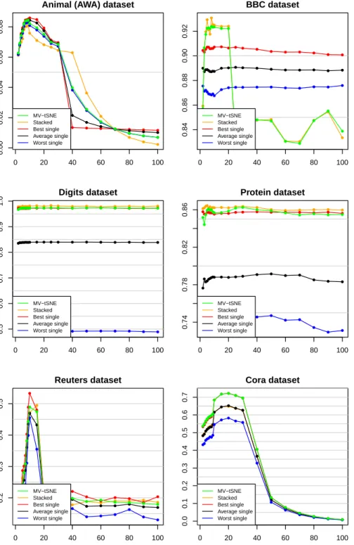
reduction methods. Taken from [107]. . . 16 3.1 MV-tSNE projection of two example datasets. . . 55 3.2 MV-tSNE dimensionality reduction evaluation with SVM

classifi-cation. . . 56 3.3 MV-tSNE dimensionality reduction evaluation with cophenetic

cor-relation (average on all input views). . . 57 3.4 MV-tSNE dimensionality reduction evaluation with area under the

RN X curve (average on all input views). . . 59

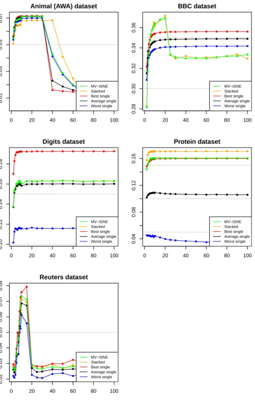
3.5 MV-tSNE clustering evaluation with clustering purity. . . 60 3.6 MV-tSNE clustering evaluation with clustering normalized mutual

information. . . 61 3.7 MV-tSNE clustering evaluation with the Davies-Bouldin index

(av-erage on all input views). Less is better. . . 62 4.1 MV-MDS projection of two example datasets. . . 71 4.2 MV-MDS dimensionality reduction evaluation with SVM

classifi-cation. . . 72 4.3 MV-MDS dimensionality reduction evaluation with cophenetic

cor-relation (average on all input views). . . 74 4.4 MV-MDS dimensionality reduction evaluation with area under the

RN X curve (average on all input views). . . 75

4.5 MV-MDS clustering evaluation with clustering purity. . . 76 4.6 MV-MDS clustering evaluation with clustering normalized mutual

information. . . 77 4.7 MV-MDS clustering evaluation with the Davies-Bouldin index

(av-erage on all input views). Less is better. . . 79 5.1 MVSC-CEV projection of two example datasets. . . 91 5.2 MVSC-CEV dimensionality reduction evaluation with SVM

(24)

xxii List of Figures

5.3 MVSC-CEV dimensionality reduction evaluation with cophenetic correlation (average on all input views). . . 94 5.4 MVSC-CEV dimensionality reduction evaluation with area under

theRN X curve (average on all input views). . . 95

5.5 MVSC-CEV clustering evaluation with clustering purity. . . 97 5.6 MVSC-CEV clustering evaluation with clustering normalized

mu-tual information. . . 98 5.7 MVSC-CEV clustering evaluation with the Davies-Bouldin index

(average on all input views). Less is better. . . 99 6.1 Dimensionality reduction evaluation with SVM classification. . . . 104 6.2 Dimensionality reduction evaluation with cophenetic correlation. . 105 6.3 Dimensionality reduction evaluation with AUC-RNX. . . 106 6.4 Clustering purity. . . 108 6.5 Clustering normalized mutual information. . . 109 6.6 Clustering evaluation with Davies-Bouldin index (less is better). . 110

(25)

Chapter 1

Multiview unsupervised

pattern recognition methods

1.1 Introduction

1.1.1 Multiview data

The development of information and communication technologies has led to ever-increasing data production in most areas of human activity. The differ-ence is not only quantitative, but it is also qualitative, as today it is relatively easy to capture different aspects or features from a given entity or experiment. New pattern recognition methods should be designed, not only to deal with large amounts of information, in the sense of high number of data samples, but also with information of heterogeneous nature even in a single dataset.

In the context of this thesis, focused on multiview datasets and methods, aview of an entity is defined as a set of variables acquired by means of an in-strument applied to the entity. In this sense, a view can be a picture, an audio or video recording, the results of a poll, survey or interview, physical variables of any kind, clinical variables, etc. Therefore, a multiview dataset is a dataset that comprises data matrices (data views) from different instruments or experiments on the same entities.

There are some concepts closely related that require a precise specification. While aviewis the most general term in this area, it actually specifies the data directly acquired from an observation instrument (camera, microphone, x-ray machine, interviewer, electronic survey, etc.). This is also known as sensory

information. On the other hand, when different characteristics are computed from a given sensory input (for example, different image descriptors from a picture), this data is usually defined as feature sets, and consequently the dataset is qualified as a multifeature dataset. It is possible to have hybrid datasets, with several sensory inputs (views) and several feature sets extracted from them.

(26)

2

CHAPTER 1. MULTIVIEW UNSUPERVISED PATTERN RECOGNITION METHODS

Finally, in the context of multimedia information management and re-trieval, it is often used the term multimodal dataset to refer to datasets that combine data from different media, like video, audio, still image, etc.

The methods presented in this thesis are generical and do not depend on a specific design or origin of the dataset, as they are conceived to process any kind of multiview, multifeature, or hybrid datasets. Throughout this thesis, the methods and the datasets used to test them will be qualified as multiview. The relevance of multiview datasets is increasing due to the high avail-ability of data acquisition instruments. However, most pattern recognition methods are designed to process a single data view. A na¨ıve option is to dis-card all data views but one; a second option is to concatenate all the input views into a single data matrix; the third option is to use a proper multi-view pattern recognition method. Many experiments have shown that the latter option renders better results [66, 62, 106, 11, 117, 106, 112, 70]. In other words, using multiview data is a challenge, as it requires new processing methods, but it is also an opportunity, as the potential results are better. As a consequence, multiview processing methods have become an important tool for data processing tasks. This is the goal of this work.

The multiview or multifeature quality is intrinsically heterogeneous, as the different aspects of the entities or subjects under study can also be heteroge-neous. Next, examples of multiview datasets are given in order to highlight this heterogeneity and to illustrate the assortment of multiview dataset designs and the varied nature of the data views.

1.1.1.1 Image datasets

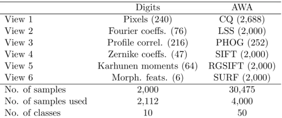
The University of California at Irvine (UCI) multiple features digits dataset [9], available at the UCI machine learning repository,1is a multifeature dataset created from a set of handwritten numerals (from ’0’ to ’9’), scanned as 15×16 grayscale pixels images. There are 200 samples of each numeral, resulting in a total of 2,000 samples. The multifeature aspect of this dataset lies in the different image descriptors that have been applied to the images. More specifically, this dataset has six feature sets: (1) the pixel averages in 2×3 windows, (2) 76 Fourier coefficients of the character shapes, (3) 216 profile correlations, (4) 64 Karhunen-Love coefficients [99], (5) 47 Zernike moments [71], and (6) 6 morphological features (not specified). As each image descriptor captures a different aspect of the images, having multiple views or feature sets of the data is assumed to contain more information about the data samples.

Strictly speaking, this is a multifeature dataset, as several features have been extracted or computed from the same sensory input (the digit images). Figure 1.1 shows an example of the original digits of this dataset.

1

(27)

1.1. INTRODUCTION 3

Figure 1.1: Example handwritten digits from the ”Multiple features” dataset.

A similar multifeature image dataset is the Animal with attributes (AWA) dataset[65]2. In this dataset the original data are 30,475 photographies of ani-mals, divided in 50 animal classes. As the input images have higher resolution than in the case of the digits dataset and they are in color, the image descrip-tors extracted from the pictures are different. However, the overall design of the dataset is the same: compute a series of image descriptors from the input images. These descriptors are: (1) 2,688 color histogram features, (2) 2,000 self-similarity features, (3) 252 pyramid histogram of oriented gradients fea-tures (PHOG) [25], (4) 2,000 scale-invariant feature transform values (SIFT) [72], (5) 2,000 colour SIFT values, and (6) 2,000 speeded-up robust features (SURF)[6]. Figure 1.2 shows an example of the original images from which the dataset has been generated.

Another source of multiview datasets are hyperspectral images, where the same location is photographed using cameras that can capture light wave-lengths other than those of visible light. A known example of this kind of datasets is the Hydice dataset 3, with a 191 band hyperspectral image of a mall in Washington DC. In this case, each band of the image can be considered a different view of the same entities, and therefore multiview methods can be useful to process it. Figure 1.3 shows some fragments of this image.

A qualitatively different multiview image dataset are the Columbia object image libraries (COIL-20 and COIL-100)[83]4, which respectively are collec-tions of pictures of 20 or 100 objects. The multiview aspect in these datasets lies in the fact that there are 72 pictures of each object in the collection, taken

2 http://attributes.kyb.tuebingen.mpg.de/ 3 https://engineering.purdue.edu/~biehl/MultiSpec/hyperspectral.html 4 http://www.cs.columbia.edu/CAVE/software/softlib/coil-20.php

(28)

4

Figure 1.2: Example images from the ”Animal with attributes” dataset. Taken from [65].

from different angles. Figure 1.4 shows an example of some of these pictures. No image descriptors are provided in this dataset, but simply the images of the objects with the backgrounds removed.

A similar dataset is the extended Yale face database B [42]5, that contains gray level images of 28 human subjects, each with 9 poses and 64 different lighting conditions. The goal of this dataset is to train face recognition sys-tems robust to varying situations. Figure 1.5 shows some example images of one of the subjects in the dataset.

1.1.1.2 Text datasets

There are multiple ways in which a text can be analyzed to extract features from it. As a consequence, there are several approaches to text multiview dataset. Some of the most well known among them are described next.

The BBC News multiview text collection [44, 43]6 comprises 2,225 news articles from the BBC news website (years 2004-2005) labelled with one of five possible topics (business, entertainment, politics, sport or tech). There are several subsets, but the overall dataset design is to split each news article in segments (ranging from 2 to 4) and use each of the segments as a different data view. The features of a segment are the non-stop words it contains. The

5

http://vision.ucsd.edu/~leekc/ExtYaleDatabase/ExtYaleB.html

6

(29)

1.1. INTRODUCTION 5

Figure 1.3: Example fragments from the Hydice dataset. Taken from [69].

complete feature matrix of each view is a matrix of documents×words.

A different approach to build multiview datasets is exemplified by the Reuters multilingual corpus [3]7, a set of 18,758 news articles labelled in six categories. In this case the multiview aspect lies in the fact that these articles are available in five different languages (English, French, German, Italian and Spanish).

7

https://archive.ics.uci.edu/ml/datasets/Reuters+RCV1+RCV2+Multilingual+ Multiview+Text+Categorization+Test+collection

(30)

6

Figure 1.4: Example images from the COIL-20 dataset.

Figure 1.5: Example images from one subject in the extended Yale face database B.

(31)

1.1. INTRODUCTION 7

Figure 1.6: Excerpt from the phenotypic data in the ALL dataset.

The Citeseer dataset [73]8 consists of 3,312 scientific publications from the Citeseer database [10] labelled with one of six classes according to their subject area. It features two data views: (1) a binary dictionary of 3,703 words, where each publication has a 1 if it contains the word or a 0 otherwise, and (2) a symmetrical citation network, as a matrix of 3,312×3,312 elements whose value cij = 1 if documenticites documentj or vice versa, orcij = 0 if there

are no references between these documents. In this case, the dictionary view is defined in feature space while the citation view is defined in graph space.

There exist several datasets with the same structure, as for example the Cora dataset [79], which contains 2,708 scientific publications classified into one of seven classes. This dataset also has two views, one bag of words with 1,433 words and a reference graph that represents 5,429 links between docu-ments.

WebKB [24] has a similar structure, but the source data are the words in web pages from four universities and their hyperlinks.

1.1.1.3 Biological datasets

Biology, medicine and related areas are also a natural source of multiview data, as the subjects themselves are of complex nature and there are numer-ous kinds of tests and instruments that produce different data. Some examples of these datasets are presented next.

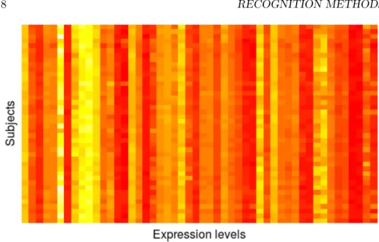
The acute lymphocytic leukemia dataset (ALL) [18] 9 compiles informa-tion from 128 subjects. One of the views includes 21 phenotypic features (age, gender, including biological markers and clinical diagnosis). The other view has the expression level of 12,625 genes. Figures 1.6 and 1.7 illustrate the two views of this dataset.

8

http://www.cs.umd.edu/~sen/lbc-proj/LBC.html

9

(32)

8

Figure 1.7: Partial heatmap of the gene expression data in the ALL dataset.

The Berkeley protein dataset for genomic data fusion [66]10is a multiview dataset whose samples are 1,040 yeast proteins. The proteins are labeled according to their location, as either membrane proteins, ribosomal proteins, or other. This dataset comprises 8 data views or feature sets, intended to grant knowledge on different aspects of the proteins so as to improve the predictive power of machine learning methods. The 8 views of this dataset are:

• KSW: Smith-Waterman[93] distance kernel on protein sequences.

• KB: BLAST[2] distance kernel on protein sequences.

• KPfam: Pfam database [95] hidden markov model kernel on protein

se-quences.

• KFFT: fast fourier transform of the hydrophobicity profile [64] extracted

from the protein sequences. Useful to recognize membrane proteins.

• KLI: linear kernel on protein interactions.

• KD: diffusion kernel on protein interactions.

• KE: radial basis kernel on gene expression (microarray gene expression

on 441 genes).

• KRND: linear kernel on a matrix of random numbers, used as baseline

to compare the other kernels.

10

(33)

1.1. INTRODUCTION 9

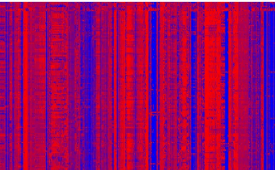
Figure 1.8: Expression profiles of the ribosomal genes. Rows correspond to the ribosomal genes, and columns to the microarray experiments. Taken from [66]

.

An important aspect of these data views is that some are defined in feature space (for example the expression levels) while others are relationships between proteins and therefore are defined in graph space. Also, as the focus of [66] is to present different kernel methods, some of the feature sets are different kernel matrices of the same data (protein sequences or interactions). Strictly speaking, this is a multiview dataset, as three different views of the proteins are used (sequences, interactions, expression), and also a multifeature dataset, as several features are extracted from the original views (the different kernels applied).

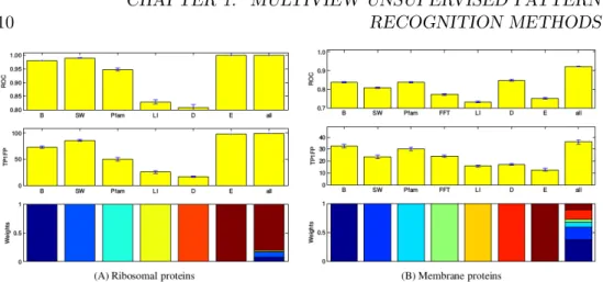
Figure 1.8 shows the expression profiles of the ribosomal genes. Figure 1.9 shows the improvement on classification accuracy of using all the data views relative to using only one view.

1.1.1.4 Multimodal datasets

Multimodal datasets combine information from different media sources, such as image and audio, in order to increase the amount of information available to the learning methods.

(34)

10

Figure 1.9: Comparison of single-view versus multiview classification. The first row shows the ROC classification score. The second row shows the per-centage of true positives at one percent false positives. The third row shows the relative weights of the kernel matrices for the linear combination used in the experiments. Taken from [66].

The Wikipedia articles cross-modal dataset [22]11 contains both images and texts from 2,866 Wikipedia articles, classified into one of ten categories. This dataset is designed to test cross-modal multimedia retrieval methods, where information from a single view is deemed insufficient for the task and the combination of the different views is expected to increase the quality of the results.

There exist several datasets composed of images and their associated anno-tation tags. Among the most popular in the literature are: Corel5k [34], that contains 5,000 images from a Corel image CD that are manually annotated with different tags; ESP Game [105], that includes 20,000 images extracted from the profiles of the users of an online game, along with user-defined textual information; and NUS-WIDE [19]12, that contains 269,648 extracted from the social network Flickr, along with six image feature sets, and the ground truth for 81 concepts or tags, where a given image can have more than one concept. Figure 1.10 shows some example images and their tags from the NUS-WIDE dataset.

11

http://www.cs.umd.edu/~sen/lbc-proj/LBC.html

12

(35)

1.1. INTRODUCTION 11

Figure 1.10: Example figures and tags from NUS-WIDE dataset. Taken from [17].

1.1.2 Unsupervised pattern recognition methods

”Development of unsupervised pattern recognition methods is the most challenging and promising area of research today.” Andrew Ng, NIPS Conference, Dec. 2016

Pattern recognition methods can be classified in two categories: supervised and unsupervised. Supervised methods require the existence of some kind of data sample labeling that indicates the class or other relevant property of each sample. Building labeled datasets is usually expensive, as in most cases a human expert (or a team of them) is required to generate the labeling. This limits the number of samples that can be labeled by the availability of human experts, usually in the thousands of samples. Moreover, labeling a dataset can be intrinsically difficult or laborious, as in image partition tasks where each object in the image has to be isolated, for example by drawing its contour, or in medical diagnosis.

It is important to note that the nature of the labels depends on the task that has to be solved. For example, on image processing there are numerous tasks to be performed: image segmentation, identification of a specific object type, identification of letters or digits, of faces, car models, etc. In each case, the labeling will be different, even if the image set is the same.

Nowadays, in the era of the big data, it is possible to acquire millions or even billions of data samples more easily than it has ever been. But in most cases, this data is not labeled. In general, manually labeling millions of data samples is unaffordable. Although hybrid methods exist that can use partially labeled data, known as semi-supervised methods, they are not always suitable. Unsupervised methods do not require any kind of human annotation on the data in order to perform their pattern recognition tasks. Two of the most relevant unsupervised pattern recognition tasks are dimensionality reduction and data clustering.

(36)

12

1.1.2.1 Dimensionality reduction

Dimensionality reduction methods, also known as data embedding methods or data projection methods, have as their goal to transform an input dataset with high dimensionality (i.e. high number of variables), into a lower dimen-sionality space, i.e. with fewer variables. This process must keep as much information as possible from the original dataset. Application of dimension-ality reduction methods often is one of the first steps in the data analysis workflow. The dimensionality reduction offers several advantages: it gives researchers a better understanding of the data, it sometimes improves the usefulness of the data (removing noise or irrelevant information), and it also reduces the computational complexity of the next data processing steps.

Some dimensionality reduction methods, also called data projection meth-ods, are specifically designed to generate a graphical representation of high dimensional data. Reducing the data to a 2 or 3-dimensional space allows to graphically display the data, giving researchers an insight into the structure of the data that may be difficult to attain otherwise.

Among the most relevant dimensionality reduction methods are: principal components analysis (PCA)[53], multidimensional scaling (MDS) [60, 61, 23], t-distributed stochastic neighbour embedding (t-SNE) [102, 74, 75, 76], canon-ical correlation analysis (CCA)[46, 47].

1.1.2.2 Clustering algorithms

The goal of clustering algorithms is to find groups or clusters of samples given a data set of which no previous information about groups or classes is assumed. This is one of the first steps when analyzing new data, as it suggests a structure for initially unstructured data.

Most clustering algorithm have a parameter that controls the granularity of the clustering, be it the number of clusters to be obtained, the minimum distance to group two points together, or any other equivalent granularity controlling parameter. There is no single solution of the clustering of a dataset, but rather it can be done at different levels of detail or granularity.

There is a wide range of clustering algorithms of which some representa-tive examples are: K-means[48, 81], hierarchical clustering[52, 82], partition around medoids (PAM)[59, 31], DBScan [35], spectral clustering[87, 84].

1.2 State of the art: multiview dimensionality

reduction

The goal of multiview dimensionality reduction methods is to reduce a dataset with multiple, high-dimensional data views {X1, X2, . . . Xv} into a single,

lower-dimensional space or data projection, while keeping the most relevant properties of the original data.

(37)

1.2. STATE OF THE ART: MULTIVIEW DIMENSIONALITY

REDUCTION 13

In general, dimensionality reduction methods are expected to preserve the relative distances between the data samples. This is a relatively difficult prob-lem to solve with a single data view, and it obviously becomes harder to solve when there are several data views, as the distances between data samples may vary from view to view and a consensus solution must be found.

When analyzing single-view dimensionality reduction methods, the qual-ity of the resulting data space with respect to the original data is analyzed from two points of view. First, the local data structure is evaluated: do the points in the low-dimensional space have the same neighbours as in the original, high-dimensional space? A method whose projections satisfy this condition are said to keep the local data structure. However, this is not the only desirable property of a dimensionality reduction method, as there is a second question to be assessed: if points a and b are far from each other in the input space, are they also far from each other in the output space? This is also an important feature, and the methods that satisfy it are said to preserve

the global data structure.

These two properties (preservation of local and global data structure) are also central to multiview dimensionality reduction methods, with the added difficulty of greater computational complexity and potential conflicts between views. A nave solution to this problem is to concatenate the input views into a single feature matrix, but this method does not account for the intrinsic structure of each data view and therefore does not fully exploit the richness of the multiview data.

1.2.1 Multiview dimensionality reduction methods

1.2.1.1 Low-rank approximation methods

Laplacian eigenmaps[7], also known as spectral embedding, is a well known single-view dimensionality reduction method. Multiview spectral embedding (MSE)[108] is an extension of spectral embedding to multiview datasets. Its goal is to find a low-dimensional and smooth embedding of the high-dimensional, multiple input views. More specifically, if the multiview dataset X is com-posed of V data matrices such that X = {X(v) ∈ _Rn×mv_}_, _∀ ₁ _≤ _v _≤ _V_,

then the resulting low-dimensional representation of X is Y ∈Rn×d, whered

is a user defined parameter such that d < mv ∀1 ≤v ≤ V. In other words,

the dimensionality of the low-dimensional representation has to be lower than the dimensionality of any of the input views. MSE comprises three steps: part optimization, global coordinate alignment, and alternating optimization. The first stage, part optimization, is based on the patch alignment frame-work described in [116]. The goal of this stage is to independently obtain a low-dimensional representation of each view that preserves the locality of each sample, i.e. the relationship with its closest neighbours. In order to find the patch of the i-th sample in the v-th view, denoted as X_i(v), the following

(38)

14

objective function has to be minimized

min Y={Y_i(v)},α V X v=1 αvtr Y_i(v)L(_iv)Y_i(v)T (1.1)

whereY_i(v)is the low-dimensional representation ofX_i(v),L(_iv)is the Laplacian of X_i(v), andαv is a weight value associated to each view that increases with

the relative relevance of viewv.

On the second stage, the different low-dimensional representations Y(v)

are aligned by assuming that they can be unified from the global coordinate matrixY by means of a selection matrix that encodes the spatial relationship with the samples in the high dimensional space, such that Y_j(v) =Y S_j(v). In other words, the low-dimensional representations of each view are consistent with each other globally. The solution to these transformations is given by the following objective function

min Y,α V X v=1 αr_vtrY L(_nv)YT s.t. Y YT =I; V X v=1 αv = 1; αv ≥0 (1.2)

The third and last stage of MSE is an alternating optimization algorithm that minimizes the previous objective function in a computationally efficient way. MatrixY is the resulting global low-dimensional projection.

The method described in [88] aims at generating a common, low-dimensional projection of several data views. The goal is to apply this projection with cross-media document retrieval, looking for the nearest neighbours in the pro-jection space, saving time and memory. Their premise is to make two samples appear close to each other in the projection if and only if they are close in all the input views. In order to obtain the common projection, a projection func-tion is defined for each data view such that (two view case, such as described in the paper; it can be extended to more views):

g1 :Rd1 →RD and g2:Rd2 →RD (1.3)

where di is the dimensionality of view i and D is the dimensionality of the

desired common projection; in general it is assumed D max(d1, d2). A linear parametrization of the above functions is assumed, such that g₁w :=

hw1, φ(xi)i and g2w := hw2, ψ(yi)i. Functions g1 and g2 are determined by optimizing the following objective function

(39)

1.2. STATE OF THE ART: MULTIVIEW DIMENSIONALITY REDUCTION 15 L(w1, w2,X,Y,S) := m X i,j=1 Li,j(w1, w2, xi, yj,Sxi) +ηΩ(w1) +γΩ(w2) (1.4)

where the loss function L is defined as follows

Li,j(w1, w2, xi, yj,Sxi) = Iyj∈S_xi 2 ×L i,j 1 + 1−Iyj∈S_xi 2 ×L i,j 2 (1.5) with Li,j₁ =kgw1 1 (xi)−g2w2(yj)k2F (1.6) Li,j₂ (βd) =          −1 2β 2 d+aλ 2 2 , if 0≤ |βd|< λ |βd|2₋₂_aλ_|_β_d|₊_a2_λ2 2(a−1) , if λ≤ |βd| ≤aλ 0, if |βd| ≥aλ (1.7)

where aand λare heuristically chosen constants. This optimization problem is further decomposed in two lesser problems and resolver iteratively. The resulting projection functions g1 and g2 can then be used to generated the desired common projection.

The convex multi-view subspace learning method (MSL) [107] aims at learning a subspace representation of a multiview dataset while assuming and enforcing conditional independence between the different views. A convex regularizer that finds the subspace is proposed. This method is also designed to achieve the best possible reconstruction of the original data from the low-dimensional representation. Summarizing the method, it applies an optimiza-tion algorithm to the objective funcoptimiza-tion

min

K∈convGf(K), f(K) =k

ˆ

Z−Kk2_F (1.8)

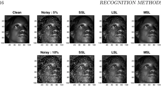
where K is the desired low-dimensional representation, convG is the convex hull of the set of possible subspaces for the input views, ˆZ =CH is the prod-uct of the concatenated feature matrixCand its common 2,1-normH. Figure 1.11 compares the quality of an image reconstructed using MSL with respect to the same image reconstructed using two alternative methods: local mul-tiview subspace learning (LSL) [88] and single-view subspace learning (SSL) [13].

(40)

16

Figure 1.11: Reconstructed image comparison between different dimensional-ity reduction methods. Taken from [107].

The ensemble manifold regularized sparse low-rank approximation (EMR-SLRA) algorithm [114] uses the framework of least-squares component analysis [27] to obtain a low-rank approximation of the concatenated multiview feature matrix. This algorithm comprises three steps: first it computes the low-rank approximation of the multiview matrix, second it regularizes the ensemble manifold, and finally it determines and applies a group sparsity constraint.

LetX ={X1, X2, . . . XV}be the concatenated feature matrix. The low-rank

approximationY of X is given by the following expression

min

U,Y kX−U Yk

2

s.t. UTU =I

(1.9)

On the second step, the low-rank approximation Y obtained has to be regularized, as from its definition all the features in X have been processed uniformly, and the intrinsic structure of each of the input views has not been considered. EMR-SLRA uses ensemble manifold regularization [41] and heat kernels [7] to find a vector of view coefficients β = {β1, β2, . . . , βV}, so that

input viewXiis multiplied by that factor in order to account for their different

(41)

1.2. STATE OF THE ART: MULTIVIEW DIMENSIONALITY REDUCTION 17 min Y,β V X v=1 (βv)rtr(Y L(v)YT) s.t. V X v=1 βi = 1, βv >0 (1.10)

where L(i) _{is the Laplacian matrix of input view} _X

i and r is a user defined

parameter. Finally, a group sparsity constraint is introduced in order to min-imize the potential noise introduced in Y from X. To minimize the effects of that noise, an ideal multiview feature matrix ˆX is obtained by applying the

`2,1-norm fitting constraint [85], as it is robust against noise in the data [109]. The expression to compute ˆX is

min ˆ X

kXˆ −Xk2,1 (1.11)

The`2,1-norm regularized is defined as: kXk2,1 = X i s X j X_ij2 =X i kxi,:k2 (1.12)

ReplacingX by ˆX in Equation 1.9 along a number of iterations produces a low-rank projection matrix Y that is more robust to the noise in the input views.

Multitask multiview feature embedding (MMFE) [115] generates a low-rank approximation matrix to the multiview data. The overall structure of the method is similar to that of EMR-SLRA [114], although the integration of the multiview data is now based on multitask learning methods [14, 36, 86, 33]. More specifically, each input data view is considered a different learning task. The objective function used to find the integrated low-rank representation Y

is min U,U(v)_,Y,Y(v)kX−U Yk 2₊ V X v=1 kX(v)−U(v)Y(v)k2 +α V X v=1 kY −Y(v)k2 s.t. UTU =I, U(v)TU(v) =I (1.13)

where {X1, X2, . . . XV} are the input views, X is the concatenated feature

matrix, Y(v) is the low-rank representation of X(v), Y is the low-rank repre-sentation of X,U(v) and U are the projection of the data points into the cor-responding low-rank space, and α is a regularization user defined parameter.

(42)

18

The resulting low-rank matrixY is the desired low-dimensional representation of the original data.

1.2.1.2 Probabilistic methods

The multiview stochastic neighbor embedding method (m-SNE) [110] is a multiview method based on stochastic neighbor embedding (SNE) [49] and t-distributed SNE (t-SNE) [102, 74]. t-SNE computes a symmetric joint prob-ability distribution from the pairwise distances of the data samples. The con-ditional probability between points xi and xj in the input high-dimensional

space is pj|i = exp(−kxi−xjk2/2σ2) P k6=l exp(−kxk−xlk2/2σ2) (1.14)

whereσis an hyperparameter of the method. The symmetric joint probability distribution, designed to avoid the effect of outlier points, is pij =

pj|i+pi|j

2n ,

wherenis the number of data samples. m-SNE generates one symmetric joint probability matrix for each input view and combines them using the next formula pij = V X v=1 α(v)p(_ijv) (1.15)

whereα(v) is a coefficient associated with each view andp(_ijv) is the joint prob-ability matrix of viewv. This produces a single joint probability matrix that is used as input for the standard t-SNE method.

1.2.1.3 Kernel-based methods

The kernelized multiview projection (KMP) [91] is a kernel method to reduce a multiview dataset of human actions, where each frame of a video capture of a subject performing an action is a view of the dataset. The approach of this method is to use a kernel that reduces the multiple, high-dimensional input views (video frames) to a single, low-dimensional space. Another requisite of this method is that it should be computationally efficient. The method comprises three steps. First, it applies an image filter called incremental nave Bayes filter (INBF) to remove the noise in the frames and try to keep only the information relevant to the task. This step is specific to the human action recognition problem. Second, it computes a kernel matrix for each input view using dynamic time warping (DTW)[8] using the following kernel function between videosvp and vq in view i:

(43)

1.2. STATE OF THE ART: MULTIVIEW DIMENSIONALITY REDUCTION 19 ki(vp, vq) = exp −DTW(X i p, Xqi)2 2σ2 (1.16) this produces a set of kernel matricesK1, K2, . . . , KM, whereM is the number

of views. After computing the Laplacian of these kernel matrices,L1, L2, . . . , LM,

an iterative procedure is applied to compute the fused kernel matrix K = PM

i=1αIKi and the fused Laplacian matrix L =PMi=1αILi. The coefficients

initially are αi = _M1 1 ≤ i ≤M, but are iteratively adjusted by solving the

generalized eigenvalue problem

KLKp =λKDKp (1.17)

where Dis the diagonal matrix ofKp. This process is repeated until Kp and

αi become stable; the final common projection P is derived from the stable

value of Kp.

1.2.1.4 Co-training methods

The method presented in [111] is specifically designed to improve image tag-ging and classification. It assumes a two-view dataset, with images as one view and annotation tags as the other. From the image view, several feature sets can be extracted using different image descriptors. The main strategy of this method is to have the information on each view guide the information extraction from the other view, in order to obtain an improved set of image tags. In the end, an improved common subspaceZ is obtained, on which the image tags are predicted. First, the geometric structure of the different views is modeled by a corresponding k-nearest neighbour graph {Wv}V

v=1, where

V is the number of image feature views. WS = TTT is used to model the semantic structure of the images, where T is the matrix of image tags. The common subspace Z is obtained by optimization of the following expression

min Z f(Z), s.t. Z T_Z ₌_I _(1.18) where f(Z) is defined as f(Z) = 1 γlog n_XV v=1 exp[γkZ−(WhWS)k2_F] o +ηkT −ZZTTk2_F (1.19)

where is the Hadamard product [39] and kAkF is the Frobenius norm of

matrixA. The common subspaceZ is then used to train a classifier to decide on the presence or absence of each possible image tag in the dataset.

(44)

20

1.3 State of the art: multiview clustering

In general terms, clustering a dataset with multiple data views{V1, V2, . . . Vc}

involves the following steps:

1. Obtain a similarity matrixSi for each view Vi.

2. Compute a projectionPi of eachSi into a space suitable for clustering.

3. Produce a clustering assignment.

The main structural difference between the multiview clustering methods proposed in the literature lies in the step where the information from the multiple views is collapsed into a single view in order to produce the final clustering assignment.

The first category of multiview clustering methods merges the similarity matrices to obtain a combined similarity matrixS0 that minimizes the differ-ences between the input similarity matricesSi, i.e. views are merged in Step

1. Afterwards, a standard clustering algorithm is applied to S0 in order to obtain the final clustering.

The second category of multiview clustering methods merge the input views during Step 2 to generate a compatible projection for all views (P0). Afterwards, a standard clustering method is applied to the merged projection

P0.

Ensemble clustering methods are designed to overcome the randomness of clustering methods such as K-means by combining clustering assignments from several runs in order to find a stable assignment. Although not strictly considered as multiview clustering methods, they can be used for multiview clustering if they are applied to the clustering assignments of different views. Thus, they would produce a clustering assignment compatible with all views. These methods merge the information from the different views after Step 3.

There exist several multiview clustering methods in the literature that are described next, classified according to the step where they merge the information in order to produce the final clustering assignment.

1.3.1 View merging methods

The first category of multiview clustering methods merge all the input views into a single similarity matrixS0, then apply a standard clustering algorithm to it.

The method described in [29] is designed to merge exactly two input views by minimizing the disagreement between them, applying the Minimizing-disagreement algorithm [28]. This method generates a weighted graph where each data sample is a node and the edges between nodesiand jare weighted