Optimal Solutions for Sparse Principal Component Analysis

Optimal Solutions for Sparse Principal Component Analysis

Alexandre d’Aspremont [email protected]

ORFE, Princeton University Princeton, NJ 08544, USA

Francis Bach [email protected]

INRIA - WILLOW Project-Team

Laboratoire d’Informatique de l’Ecole Normale Sup´erieure (CNRS/ENS/INRIA UMR 8548)

45 rue d’Ulm, 75230 Paris, France

Laurent El Ghaoui [email protected]

EECS Department, U.C. Berkeley Berkeley, CA 94720, USA

Editor: Aapo Hyvarinen

Abstract

Given a sample covariance matrix, we examine the problem of maximizing the variance explained by a linear combination of the input variables while constraining the number of nonzero coefficients in this combination. This is known as sparse principal component analysis and has a wide array of applications in machine learning and engineering. We formulate a new semidefinite relaxation to this problem and derive a greedy algorithm that computes a full set of good solutions for all target numbers of non zero coefficients, with total complexity O(n3), where n is the number of variables. We then use the same relaxation to derive sufficient conditions for global optimality of a solution, which can be tested in O(n3)per pattern. We discuss applications in subset selection and sparse recovery and show on artificial examples and biological data that our algorithm does provide globally optimal solutions in many cases.

Keywords: PCA, subset selection, sparse eigenvalues, sparse recovery, lasso

1. Introduction

Principal component analysis (PCA) is a classic tool for data analysis, visualization or compres-sion and has a wide range of applications throughout science and engineering. Starting from a multivariate data set, PCA finds linear combinations of the variables called principal components, corresponding to orthogonal directions maximizing variance in the data. Numerically, a full PCA involves a singular value decomposition of the data matrix.

One of the key shortcomings of PCA is that the factors are linear combinations of all original variables; that is, most of factor coefficients (or loadings) are non-zero. This means that while PCA facilitates model interpretation and visualization by concentrating the information in a few factors, the factors themselves are still constructed using all variables, hence are often hard to interpret.

factors involve only a few coordinate axes). Solutions that have only a few nonzero coefficients in the principal components are usually easier to interpret. Moreover, in some applications, nonzero coefficients have a direct cost (e.g., transaction costs in finance) hence there may be a direct trade-off between statistical fidelity and practicality. Our aim here is to efficiently derive sparse principal components, that is, a set of sparse vectors that explain a maximum amount of variance. Our belief is that in many applications, the decrease in statistical fidelity required to obtain sparse factors is small and relatively benign.

In what follows, we will focus on the problem of finding sparse factors which explain a maxi-mum amount of variance, which can be written:

max kzk≤1z

T_Σz

−ρCard(z) (1)

in the variable z_∈Rn, whereΣ_∈Sn is the (symmetric positive semi-definite) sample covariance matrix,ρis a parameter controlling sparsity, and Card(z)denotes the cardinal (or `0 norm) of z, that is, the number of non zero coefficients of z.

While PCA is numerically easy, each factor requires computing a leading eigenvector, which can be done in O(n2_{), sparse PCA is a hard combinatorial problem. In fact, Moghaddam et al. (2006b)} show that the subset selection problem for ordinary least squares, which is NP-hard (Natarajan, 1995), can be reduced to a sparse generalized eigenvalue problem, of which sparse PCA is a par-ticular intance. Sometimes factor rotation techniques are used to post-process the results from PCA and improve interpretability (see QUARTIMAX by Neuhaus and Wrigley 1954, VARIMAX by Kaiser 1958 or Jolliffe 1995 for a discussion). Another simple solution is to threshold the load-ings with small absolute value to zero (Cadima and Jolliffe, 1995). A more systematic approach to the problem arose in recent years, with various researchers proposing nonconvex algorithms (e.g., SCoTLASS by Jolliffe et al. 2003, SLRA by Zhang et al. 2002 or D.C. based methods such as (Sriperumbudur et al., 2007) which find modified principal components with zero loadings). The SPCA algorithm, which is based on the representation of PCA as a regression-type optimization problem (Zou et al., 2006), allows the application of the LASSO (Tibshirani, 1996), a penaliza-tion technique based on the`1norm. With the exception of simple thresholding, all the algorithms above require solving non convex problems. Recently also, d’Aspremont et al. (2007b) derived an

`1based semidefinite relaxation for the sparse PCA problem (1) with a complexity of O(n4√log n) for a givenρ. Finally, Moghaddam et al. (2006a) used greedy search and branch-and-bound meth-ods to solve small instances of problem (1) exactly and get good solutions for larger ones. Each step of this greedy algorithm has complexity O(n3_{), leading to a total complexity of O(n}4_{)for a full set} of solutions. Moghaddam et al. (2007) improve this bound in the regression/discrimination case.

Our contribution here is twofold. We first derive a greedy algorithm for computing a full set of good solutions (one for each target sparsity between 1 and n) at a total numerical cost of O(n3_)based on the convexity of the of the largest eigenvalue of a symmetric matrix. We then derive tractable sufficient conditions for a vector z to be a global optimum of (1). This means in practice that, given a vector z with support I, we can test if z is a globally optimal solution to problem (1) by performing a few binary search iterations to solve a one dimensional convex minimization problem. In fact, we can take any sparsity pattern candidate from any algorithm and test its optimality. This paper builds on the earlier conference version (d’Aspremont et al., 2007a), providing new and simpler conditions for optimality and describing applications to subset selection and sparse recovery.

Cand`es and Tao 2005, Donoho and Tanner 2005 or Meinshausen and Yu 2006 among others) that there is in fact a deep connection between `0 constrained extremal eigenvalues and LASSO type variable selection algorithms. Sufficient conditions based on sparse eigenvalues (also called re-stricted isometry constants in Cand`es and Tao 2005) guarantee consistent variable selection (in the LASSO case) or sparse recovery (in the decoding problem). The results we derive here produce upper bounds on sparse extremal eigenvalues and can thus be used to prove consistency in LASSO estimation, prove perfect recovery in sparse recovery problems, or prove that a particular solution of the subset selection problem is optimal. Of course, our conditions are only sufficient, not necessary and the duality bounds we produce on sparse extremal eigenvalues cannot always be tight, but we observe that the duality gap is often small.

The paper is organized as follows. We begin by formulating the sparse PCA problem in Section 2. In Section 3, we write an efficient algorithm for computing a full set of candidate solutions to problem (1) with total complexity O(n3_{). In Section 4 we then formulate a convex relaxation} for the sparse PCA problem, which we use in Section 5 to derive tractable sufficient conditions for the global optimality of a particular sparsity pattern. In Section 6 we detail applications to subset selection, sparse recovery and variable selection. Finally, in Section 7, we test the numerical performance of these results.

1.1 Notation

For a vector z_∈R, we let_kz_k1=∑ni=1|zi|andkzk= ∑ni=1z2i

1/2

, Card(z)is the cardinality of z, that is, the number of nonzero coefficients of z, while the support I of z is the set{i : zi 6=0}and we use Icto denote its complement. Forβ_∈R, we writeβ+=max{β,0}and for X ∈Sn(the set of symmetric matrix of size n_×n) with eigenvaluesλi, Tr(X)+=∑i=n 1max{λi,0}. The vector of all ones is written 1, while the identity matrix is written I. The diagonal matrix with the vector u on the diagonal is written diag(u).

2. Sparse PCA

LetΣ∈Snbe a symmetric matrix. We consider the following sparse PCA problem:

φ(ρ)_≡ max kzk≤1z

T_Σz

−ρCard(z) (2)

in the variable z∈Rn whereρ>0 is a parameter controlling sparsity. We assume without loss of generality thatΣ_∈Sn is positive semidefinite and that the n variables are ordered by decreasing marginal variances, that is, thatΣ11≥. . .≥Σnn. We also assume that we are given a square root A of the matrixΣwithΣ=ATA, where A∈Rn×nand we denote by a1, . . . ,an∈Rnthe columns of A. Note that the problem and our algorithms are invariant by permutations ofΣand by the choice of square root A. In practice, we are very often given the data matrix A instead of the covarianceΣ.

A problem that is directly related to (2) is that of computing a cardinality constrained maximum eigenvalue, by solving:

maximize zTΣz

subject to Card(z)_≤k

kz_k=1,

in the variable z∈Rn. Of course, this problem and (2) are related. By duality, an upper bound on the optimal value of (3) is given by:

inf

ρ∈Pφ(ρ) +ρk.

where P is the set of penalty values for whichφ(ρ) has been computed. This means in particular that if a point z is provably optimal for (2), it is also globally optimum for (3) with k=Card(z).

We now begin by reformulating (2) as a relatively simple convex maximization problem. Sup-pose thatρ_≥Σ11. Since zTΣz_≤Σ11(∑n

i=1|zi|)2and(∑n_i=1|zi|)2≤ kzk2Card(z)for all z∈Rn, we have:

φ(ρ) =max_kz_k≤1zTΣz−ρCard(z)

≤(Σ11−ρ)Card(z)

≤0,

hence the optimal solution to (2) whenρ_≥Σ11is z=0. From now on, we assumeρ≤Σ11in which case the inequality_kz_{k ≤}1 is tight. We can represent the sparsity pattern of a vector z by a vector u_{∈ {}0,1_}nand rewrite (2) in the equivalent form:

φ(ρ) = max

u∈{0,1}nλmax(diag(u)Σdiag(u))−ρ1

T_u

= max

u∈{0,1}nλmax(diag(u)A

T_{A diag(u))}

−ρ1Tu

= max

u∈{0,1}nλmax(A diag(u)A

T₎

−ρ1Tu,

using the fact that diag(u)2_{=diag(u) for all variables u∈ {0,1}}n _{and that for any matrix B,}

λmax(BT_{B) =}λ_max(BBT_{). We then have:}

φ(ρ) = max

u∈{0,1}nλmax(A diag(u)A

T₎

−ρ1Tu

=max

kxk=1 u∈{max0,1}nx

T_{A diag(u)A}T_x

−ρ1Tu

=max

kxk=1 u∈{max0,1}n

n

∑

ui((aTi x)2−ρ).

Hence we finally get, after maximizing in u (and using max_v∈{0,1}βv=β+):

φ(ρ) =max kxk=1

n

∑

((aT_i x)2₋ρ)+, (4)

which is a nonconvex problem in the variable x_∈Rn. We then select variables i such that(aT i x)2−

ρ>0. Note that ifΣii=aTi ai<ρ, we must have(aTi x)2≤ kaik2kxk2<ρhence variable i will never be part of the optimal subset and we can remove it.

3. Greedy Solutions

3.1 Sorting and Thresholding

The simplest ranking algorithm is to sort the diagonal of the matrix Σand rank the variables by variance. This works intuitively because the diagonal is a rough proxy for the eigenvalues: the Schur-Horn theorem states that the diagonal of a matrix majorizes its eigenvalues (Horn and John-son, 1985); sorting costs O(n log n). Another quick solution is to compute the leading eigenvector ofΣand form a sparse vector by thresholding to zero the coefficients whose magnitude is smaller than a certain level. This can be done with cost O(n2_).

3.2 Full Greedy Solution

Following Moghaddam et al. (2006a), starting from an initial solution of cardinality one atρ=Σ11, we can update an increasing sequence of index sets Ik⊆[1,n], scanning all the remaining variables to find the index with maximum variance contribution.

Greedy Search Algorithm.

• Input:Σ_∈Rn×n

• Algorithm:

1. Preprocessing: sort variables by decreasing diagonal elements and permute elements of Σaccordingly. Compute the Cholesky decompositionΣ=AT_A.

2. Initialization: I1=_{1_}, x1=a1/_ka1_k.

3. Compute ik=argmaxi∈/Ikλmax

∑j∈Ik∪{i}aja

T j

.

4. Set Ik+1=Ik∪ {ik}and compute xk+1as the leading eigenvector of∑j∈Ik+1aja

T j. 5. Set k=k+1. If k<n go back to step 3.

• Output: sparsity patterns Ik.

At every step, Ik represents the set of nonzero elements (or sparsity pattern) of the current point and we can define zkas the solution to problem (2) given Ik, which is:

zk= argmax {zIc_k=0,kzk=1}

zTΣz₋ρk,

which means that zk is formed by padding zeros to the leading eigenvector of the submatrixΣIk,Ik.

Note that the entire algorithm can be written in terms of a factorizationΣ=ATA of the matrixΣ, which means significant computational savings whenΣis given as a Gram matrix. The matrices ΣIk,Ik and∑i∈Ikaia

T

i have the same eigenvalues and their eigenvectors are transformed of each other through the matrix A, that is, if z is an eigenvector of ΣIk,Ik, then AIkz/kAIkzkis an eigenvector of

AIkA

T Ik.

3.3 Approximate Greedy Solution

Computing n₋k eigenvalues at each iteration is costly and we can use the fact that uuT is a subgra-dient ofλmaxat X if u is a leading eigenvector of X (Boyd and Vandenberghe, 2004), to get:

λmax

∑

ajaTj

!

≥λmax

∑

ajaTj

!

which means that the variance is increasing by at least(xT

kai)2when variable i is added to Ik. This provides a lower bound on the objective which does not require finding n₋k eigenvalues at each iteration. We then derive the following algorithm:

Approximate Greedy Search Algorithm.

• Input:Σ_∈Rn×n

• Algorithm:

1. Preprocessing. Sort variables by decreasing diagonal elements and permute elements of Σaccordingly. Compute the Cholesky decompositionΣ=ATA.

2. Initialization: I1={1}, x1=a1/ka1k. 3. Compute ik=argmaxi∈/Ik(x

T kai)2

4. Set Ik+1=Ik∪ {ik}and compute xk+1as the leading eigenvector of∑j∈Ik+1aja

T j. 5. Set k=k+1. If k<n go back to step 3.

• Output: sparsity patterns Ik.

Again, at every step, Ikrepresents the set of nonzero elements (or sparsity pattern) of the current point and we can define zkas the solution to problem (2) given Ik, which is:

zk= argmax {zIc

k=0,kzk=1}

zTΣz₋ρk,

which means that zk is formed by padding zeros to the leading eigenvector of the submatrixΣIk,Ik.

Better points can be found by testing the variables corresponding to the p largest values of(xT kai)2 instead of picking only the best one.

3.4 Computational Complexity

The complexity of computing a greedy regularization path using the classic greedy algorithm in Section 3.2 is O(n4_{): at each step k, it computes (n−k) maximum eigenvalue of matrices with} size k. The approximate algorithm in Section 3.3 computes a full path in O(n3_{): the first Cholesky} decomposition is O(n3_{), while the complexity of the k-th iteration is O(k}2_{)for the maximum} eigen-value problem and O(n2_{) for computing all products(x}T_a

j). Also, when the matrixΣis directly

given as a Gram matrix ATA with A_∈Rq×nwith q<n, it is advantageous to use A directly as the square root of Σand the total complexity of getting the path up to cardinality p is then reduced to O(p3+p2n)(which is O(p3_{)for the eigenvalue problems and O(p}2_{n)for computing the vector} products).

4. Convex Relaxation

In Section 2, we showed that the original sparse PCA problem (2) could also be written as in (4):

φ(ρ) =max kxk=1

n

∑

Because the variable x appears solely through X =xxT, we can reformulate the problem in terms of X only, using the fact that when_kx_k=1, X=xxTis equivalent to Tr(X) =1, X0 and Rank(X) = 1. We thus rewrite (4) as:

φ(ρ) = max. ∑n_i=1(aT

i X ai−ρ)+

s.t. Tr(X) =1, Rank(X) =1 X0.

Note that because we are maximizing a convex function over the convex set (spectahedron) ∆n=

{X_∈Sn: Tr(X) =1,X0}, the solution must be an extreme point of∆n(i.e., a rank one matrix), hence we can drop the rank constraint here. Unfortunately, X 7→(aT

i X ai−ρ)+, the function we are maximizing, is convex in X and not concave, which means that the above problem is still hard. However, we show below that on rank one elements of∆n, it is also equal to a concave function of X , and we use this to produce a semidefinite relaxation of problem (2).

Proposition 1 Let A_∈Rn×n,ρ_≥0 and denote by a1, . . . ,an∈Rnthe columns of A, an upper bound on:

φ(ρ) = max. ∑n_i=1(aT

i X ai−ρ)+

s.t. Tr(X) =1,X 0, Rank(X) =1

can be computed by solving

ψ(ρ) = max. ∑n_i=1Tr(X1/2_B iX1/2)+

s.t. Tr(X) =1,X 0. (5)

in the variables X_∈Sn, where Bi=aiaTi −ρI, or also:

ψ(ρ) = max. ∑n_i=1Tr(PiBi)

s.t. Tr(X) =1, X0, XPi0,

(6)

which is a semidefinite program in the variables X_∈Sn, Pi∈Sn.

Proof We let X1/2_{denote the positive square root (i.e., with nonnegative eigenvalues) of a symmetric} positive semi-definite matrix X . In particular, if X=xxTwith_kx_k=1, then X1/2=X=xxT, and for allβ_∈R,βxxT has one eigenvalue equal toβand n₋1 equal to 0, which implies Tr(βxxT)+=β+. We thus get:

(aT

i X ai−ρ)+ = Tr((aiTxxTai−ρ)xxT)+ = Tr(x(xT_a

iaTi x−ρ)xT)+

= Tr(X1/2aiaiTX1/2−ρX)+=Tr(X1/2(aiaTi −ρI)X1/2)+.

For any symmetric matrix B, the function X_7→Tr(X1/2_BX1/2₎

+is concave on the set of symmetric positive semidefinite matrices, because we can write it as:

Tr(X1/2_BX1/2₎

+ = max

{0PX}Tr(PB)

= min

where this last expression is a concave function of X as a pointwise minimum of affine functions. We can now relax the original problem into a convex optimization problem by simply dropping the rank constraint, to get:

ψ(ρ)_≡ max. ∑n_i=1Tr(X1/2_a

iaTi X1/2−ρX)+ s.t. Tr(X) =1,X 0,

which is a convex program in X _∈Sn. Note that because Bi has at most one nonnegative eigen-value, we can replace Tr(X1/2_a

iaTi X1/2−ρX)+ by λmax(X1/2aiaTi X1/2−ρX)+ in the above pro-gram. Using the representation of Tr(X1/2_BX1/2₎

+detailed above, problem (5) can be written as a semidefinite program:

ψ(ρ) = max. ∑n_i=1Tr(PiBi)

s.t. Tr(X) =1,X0,XPi0,

in the variables X_∈Sn, Pi∈Sn, which is the desired result.

Note that we always haveψ(ρ)_≥φ(ρ)and when the solution to the above semidefinite program has rank one,ψ(ρ) =φ(ρ)and the semidefinite relaxation (6) is tight. This simple fact allows us to derive sufficient global optimality conditions for the original sparse PCA problem.

5. Optimality Conditions

In this section, we derive necessary and sufficient conditions to test the optimality of solutions to the relaxations obtained in Sections 3, as well as sufficient condition for the tightness of the semidefinite relaxation in (6).

5.1 Dual Problem and Optimality Conditions

We first derive the dual problem to (6) as well as the Karush-Kuhn-Tucker (KKT) optimality con-ditions:

Lemma 2 Let A_∈Rn×n,ρ_≥0 and denote by a1, . . . ,an∈Rnthe columns of A. The dual of problem (6):

ψ(ρ) = max. ∑n_i=1Tr(PiBi)

s.t. Tr(X) =1, X0, XPi0,

in the variables X_∈Sn, Pi∈Sn, is given by:

min. λmax(∑ni=1Yi)

s.t. YiBi,Yi0, i=1, . . . ,n. (7)

in the variables Yi ∈Sn. Furthermore, the KKT optimality conditions for this pair of semidefinite programs are given by:

 



(∑n

i=1Yi)X=λmax(∑ni=1Yi)X

(X₋Pi)Yi=0,PiBi=PiYi

YiBi,Yi,X,Pi0,XPi, Tr X=1.

Proof Starting from:

max. ∑n_i=1Tr(PiBi) s.t. 0PiX

Tr(X) =1,X0,

we can form the Lagrangian as:

L(X,Pi,Yi) = n

∑

Tr(PiBi) +Tr(Yi(X−Pi))

in the variables X,Pi,Yi∈Sn, with X,Pi,Yi0 and Tr(X) =1. Maximizing L(X,Pi,Yi)in the primal variables X and Pi leads to problem (7). The KKT conditions for this primal-dual pair of SDP can be derived from Boyd and Vandenberghe (2004, p.267).

5.2 Optimality Conditions for Rank One Solutions

We now derive the KKT conditions for problem (6) for the particular case where we are given a rank one candidate solution X=xxT and need to test its optimality. These necessary and sufficient conditions for the optimality of X=xxT for the convex relaxation then provide sufficient conditions for global optimality for the non-convex problem (2).

Lemma 3 Let A_∈Rn×n,ρ_≥0 and denote by a1, . . . ,an∈Rnthe columns of A. The rank one matrix X=xxT is an optimal solution of (6) if and only if there are matrices Yi∈Sn,i=1, . . . ,n such that:

   

  

λmax(∑ni=1Yi) =∑i∈I((aTi x)2−ρ) xTYix=

(aT

ix)2−ρif i∈I 0 if i_∈Ic

YiBi,Yi0.

where Bi=aiaTi −ρI, i=1, . . . ,n and Icis the complement of the set I defined by:

max i∈/I (a

T

i x)2≤ρ≤min_i ∈I(a

T ix)2.

Furthermore, x must be a leading eigenvector of both∑_i∈IaiaiT and∑ni=1Yi.

Proof We apply Lemma 2 given X =xxT. The condition 0PixxT is equivalent to Pi=αixxT andαi∈[0,1]. The equation PiBi=XYi is then equivalent toαi(xTBix−xTYix) =0, with xTBix=

(aT

ix)2−ρand the condition(X−Pi)Yi =0 becomes xTYix(1−αi) =0. This means that xTYix=

((aT

i x)2−ρ)+ and the first-order condition in (8) becomesλmax(∑ni=1Yi) =xT(∑ni=1Yi)x. Finally, we recall from Section 2 that:

∑i∈I((aTi x)2−ρ) = max

kxk=1 u∈{max0,1}n

n

∑

ui((aTi x)2−ρ)

= max

u∈{0,1}nλmax(A diag(u)A

T₎

−ρ1Tu

The previous lemma shows that given a candidate vector x, we can test the optimality of X = xxT for the semidefinite program (5) by solving a semidefinite feasibility problem in the variables Yi ∈Sn. If this (rank one) solution xxT is indeed optimal for the semidefinite relaxation, then x must also be globally optimal for the original nonconvex combinatorial problem in (2), so the above lemma provides sufficient global optimality conditions for the combinatorial problem (2) based on the (necessary and sufficient) optimality conditions for the convex relaxation (5) given in lemma 2. In practice, we are only given a sparsity pattern I (using the results of Section 3 for example) rather than the vector x, but Lemma 3 also shows that given I, we can get the vector x as the leading eigenvector of∑_i∈IaiaTi .

The next result provides more refined conditions under which such a pair(I,x)is optimal for some value of the penaltyρ>0 based on a local optimality argument. In particular, they allow us to fully specify the dual variables Yifor i∈I.

Proposition 4 Let A_∈Rn×n,ρ_≥0 and denote by a1, . . . ,an∈Rnthe columns of A. Let x be the largest eigenvector of∑i∈IaiaTi . Let I be such that:

max i∈/I (a

T

i x)2<ρ<min_i ∈I(a

T

ix)2, (9)

the matrix X=xxT is optimal for problem (6) if and only if there are matrices Yi∈Snsatisfying

λmax

∑

BixxTBi xT_B

ix

+

∑

i∈Ic

Yi

!

≤

∑

i∈I

((aT_i x)2₋ρ),

with YiBi−Bixx

T_B i

xT_B

ix ,Yi0, where Bi=aia

T

i −ρI, i=1, . . . ,n.

Proof We first prove the necessary condition by computing a first order expansion of the functions Fi: X 7→Tr(X1/2BiX1/2)+ around X =xxT. The expansion is based on the results in Appendix A which show how to compute derivatives of eigenvalues and projections on eigensubspaces. More precisely, Lemma 10 states that if xT_{Bx>0, then, for any Y 0:}

Fi((1−t)xxT+tY) =Fi(xxT) + t xT_B

ix

Tr BixxTBi(Y−xxT) +O(t3/2),

while if xT_{Bx<0, then, for any Y 0,:}

Fi((1−t)xxT+tY) =t+Tr

Y1/2

Bi−

BixxTBi xT_B

ix

Y1/2

+

+O(t3/2_).

Thus if X=xxT is a global maximum of∑iFi(X), then this first order expansion must reflect the fact that it is also local maximum, that is, for all Y_∈Snsuch that Y0 and TrY =1, we must have:

lim t→0+

1 t

n

∑

[Fi((1−t)xxT+tY)−Fi(xxT)]≤0,

which is equivalent to:

−

∑

i_∈I

xTBix+TrY

∑

BixxTBi xT_B

ix

!

+

∑

i_∈Ic

Tr

Y1/2

Bi−

BixxTBi xT_B

ix

Y1/2

Thus if X=xxT is optimal, withσ=∑_i∈IxTBix, we get:

max

Y0,TrY=1TrY

∑

BixxTBi xT_B

ix −

σI

!

+

∑

i_∈Ic

Tr

Y1/2 Bi−Bix(xTBix)†xTBi

Y1/2

+≤0

which is also in dual form (using the same techniques as in the proof of Proposition 1):

min {YiBi−BixxT Bi

xT Bix ,Yi0}

λmax

∑

BixxTBi xT_B

ix

+

∑

i∈Ic

Yi

!

≤σ,

which leads to the necessary condition. In order to prove sufficiency, the only non trivial condition to check in Lemma 3 is that xTYix=0 for i∈Ic, which is a consequence of the inequality:

xT

∑

BixxTBi xT_B

ix

+

∑

i∈Ic

Yi

!

x_≤λmax

∑

BixxTBi xT_B

ix

+

∑

i∈Ic

Yi

!

≤xT

∑

BixxTBi xT_B

ix

!

x.

This concludes the proof.

The original optimality conditions in (3) are highly degenerate in Yi and this result refines these optimality conditions by invoking the local structure. The local optimality analysis in proposition 4 gives more specific constraints on the dual variables Yi. For i∈I, Yimust be equal to BixxTBi/xTBix, while if i_∈Ic, we must have YiBi−BixxTBi/xTBix, which is a stricter condition than Yi Bi (because xTBix<0).

5.3 Efficient Optimality Conditions

The condition presented in Proposition 4 still requires solving a large semidefinite program. In practice, good candidates for Yi, i∈Iccan be found by solving for minimum trace matrices satis-fying the feasibility conditions of proposition 4. As we will see below, this can be formulated as a semidefinite program which can be solved explicitly.

Lemma 5 Let A_∈Rn×n,ρ_≥0, x_∈Rnand Bi=aiaTi −ρI with a1, . . . ,an∈Rnthe columns of A. If(aT

i x)2<ρandkxk=1, an optimal solution of the semidefinite program: minimize TrYi

subject to YiBi−Bixx

T_B i

xT_B ix , x

T_Y

ix=0,Yi0,

is given by:

Yi=max

0,ρ (a

T i ai−ρ)

(ρ₋(aT

i x)2)

(I₋xxT)aiaTi (I−xxT)

k(I₋xxT_)a ik2

. (10)

Proof Let us write Mi=Bi−Bixx

T_B i

xT_B

ix , we first compute:

aT_i Miai = (aTi ai−ρ)aTi ai−

(aT

i aiaTi x−ρaTi x)2

(aT

i x)2−ρ

= (a

T i ai−ρ)

ρ−(aT i x)2

When aT_i ai ≤ρ, the matrix Mi is negative semidefinite, because kxk=1 means aTi Mai ≤0 and xTMx=aT_i Mx=0. The solution of the minimum trace problem is then simply Yi=0. We now assume that aT_i ai>ρand first check feasibility of the candidate solution Yiin (10). By construction, we have Yi0 and Yix=0, and a short calculation shows that:

aT_iYiai = ρ

(aT

i ai−ρ)

(ρ₋(aT

i x)2)

(aT_i ai−(aTi x)2)

= aT_i Miai.

We only need to check that YiMion the subspace spanned by aiand x, for which there is equality. This means that Yi in (10) is feasible and we now check its optimality. The dual of the original semidefinite program can be written:

maximize Tr PiMi

subject to I₋Pi+νxxT 0 Pi0,

and the KKT optimality conditions for this problem are written:







Yi(I−Pi+νxxT) =0,Pi(Yi−Mi) =0, I₋Pi+νxxT0,

Pi0,Yi0,YiMi,YixxT =0, i∈Ic.

Setting Pi=YiTrYi/TrYi2andνsufficiently large makes these variables dual feasible. Because all contributions of x are zero, TrYi(Yi−Mi)is proportional to Tr aiaTi (Yi−Mi)which is equal to zero and Yiin (10) satisifies the KKT optimality conditions.

We summarize the results of this section in the theorem below, which provides sufficient opti-mality conditions on a sparsity pattern I.

Theorem 6 Let A_∈Rn×n,ρ_≥0,Σ=ATA with a1, . . . ,an∈Rnthe columns of A. Given a sparsity pattern I, setting x to be the largest eigenvector of ∑i_∈IaiaTi , if there is a ρ∗ ≥0 such that the following conditions hold:

max i∈Ic(a

T

i x)2<ρ∗<min i∈I (a

T

i x)2 and λmax n

∑

Yi

!

≤

∑

i∈I

((aT_i x)2₋ρ∗),

with the dual variables Yifor i∈Ic defined as in (10) and:

Yi=

BixxTBi xT_B

ix

, when i_∈I,

then the sparsity pattern I is globally optimal for the sparse PCA problem (2) withρ=ρ∗ and we can form an optimal solution z by solving the maximum eigenvalue problem:

z= argmax {zIc=0,kzk=1}

Proof Following proposition 4 and lemma 5, the matrices Yiare dual optimal solutions correspond-ing to the primal optimal solution X =xxT in (5). Because the primal solution has rank one, the semidefinite relaxation (6) is tight so the pattern I is optimal for (2) and Section 2 shows that z is a globally optimal solution to (2) withρ=ρ∗_.

5.4 Gap Minimization: Finding the Optimalρ

All we need now is an efficient algorithm to findρ∗ in theorem 6. As we will show below, when the dual variables Y_ic are defined as in (10), the duality gap in (2) is a convex function ofρhence, given a sparsity pattern I, we can efficiently search for the best possibleρ(which must belong to an interval) by performing a few binary search iterations.

Lemma 7 Let A_∈Rn×n,ρ_≥0,Σ=ATA with a1, . . . ,an∈Rn the columns of A. Given a sparsity pattern I, setting x to be the largest eigenvector of∑_i∈IaiaTi , with the dual variables Yi for i∈Ic defined as in (10) and:

Yi=

BixxTBi xT_B

ix

, when i_∈I.

The duality gap in (2) which is given by:

gap(ρ)_≡λmax n

∑

Yi

!

−

∑

i_∈I

((aT_i x)2₋ρ),

is a convex function ofρwhen

max i∈/I (a

T

i x)2<ρ<min_i ∈I(a

T ix)2. Proof For i_∈I and u_∈Rn, we have

uTYiu=

(uT_a

iaTi x−ρuTx)2

(aT

i x)2−ρ

,

which is a convex function ofρ(Boyd and Vandenberghe, 2004, p.73). For i_∈Ic, we can write:

ρ(aT i ai−ρ)

ρ₋(aT i x)2

=₋ρ+ (aT_i ai−(aTi x)2)

1+ (a T ix)2

ρ₋(aT i x)2

,

hence max_{0,ρ(aT

i ai−ρ)/(ρ−(aTi x)2)}is also a convex function ofρ. This means that: uTYiu=max

0,ρ (a

T i ai−ρ)

(ρ₋(aT

i x)2)

(uT_a

i−(xTu)(xTai))2

k(I₋xxT_)a ik2 is convex inρwhen i_∈Ic. We conclude that∑n_i=1uTYiu is convex, hence:

gap(ρ) = max kuk=1

n

∑

uTYiu−

∑

((aT_i x)2₋ρ)

This result shows that the set ofρfor which the pattern I is optimal must be an interval. It also suggests an efficient procedure for testing the optimality of a given pattern I. We first compute x as a leading eigenvector∑_i∈IaiaTi . We then compute an interval inρfor which x satisfies the basic consistency condition:

max i∈/I (a

T

i x)2≡ρmin≤ρ≤ρmax≡min i∈I(a

T i x)2.

Note that this interval could be empty, in which case I cannot be optimal. We then minimize gap(ρ) over the interval[ρmin,ρmax]. If the minimum is zero for someρ=ρ∗, then the pattern I is optimal for the sparse PCA problem in (2) withρ=ρ∗.

Minimizing the convex function gap(ρ) can be done very efficiently using binary search. The initial cost of forming the matrix∑n_i=1Yi, which is a simple outer matrix product, is O(n3). At each iteration of the binary search, a subgradient of gap(ρ)can then be computed by solving a maximum eigenvalue problem, at a cost of O(n2_{). This means that the complexity of finding the optimalρover} a given interval[ρmin,ρmax]is O(n2log2((ρmax−ρmin)/ε)), whereεis the target precision. Overall then, the total cost of testing the optimality of a pattern I is O(n3_+n2_log

2((ρmax−ρmin)/ε)). Note that an additional benefit of deriving explicit dual feasible points Yiis that plugging these solutions into the objective of problem (7):

min. λmax(∑ni=1Yi)

s.t. YiBi,Yi0, i=1, . . . ,n.

produces an upper bound on the optimum value of the original sparse PCA problem (2) even when the pattern I is not optimal (all we need is aρsatisfying the consistency condition).

5.5 Solution Improvements and Randomization

When these conditions are not satisfied, the relaxation (6) has an optimal solution with rank strictly larger than one, hence is not tight. At such a point, we can use a different relaxation such as DSPCA by d’Aspremont et al. (2007b) to try to get a better solution. We can also apply randomization techniques to improve the quality of the solution of problem (6) (Ben-Tal and Nemirovski, 2002).

6. Applications

In this section, we discuss some applications of sparse PCA to subset selection and compressed sensing.

6.1 Subset Selection

We consider p data points in Rn, in a data matrix X _∈Rp×n. We assume that we are given real numbers y_∈Rpto predict from X using linear regression, estimated by least squares. We are thus looking for w_∈Rnsuch that_ky₋X w_k2is minimum. In the subset selection problem, we are looking for sparse coefficients w, that is, a vector w with many zeros. We thus consider the problem:

s(k) = min w_∈Rn,Card w_≤kk

Using the sparsity pattern u∈ {0,1}n_{, and optimizing with respect to w, we have}

s(ρ) = min

u∈{0,1}n_,1T_u≤kkyk

2_−yT_X(u)(X(u)T_X(u))−1_X(u)T_y,

where X(u) =X diag(u). We can rewrite yT_X(u)(X(u)T_X(u))−1_X(u)T_{y as the largest generalized} eigenvalue of the pair(X(u)T_yyT_X(u),X(u)T_{X(u)), that is, as}

yTX(u)(X(u)TX(u))−1X(u)Ty= max w∈Rn

wTX(u)T_yyT_X(u)w wT_X(u)T_X(u)w .

We thus have:

s(k) =_ky_k2₋ max

u∈{0,1}n_,1T_u≤kwmax_∈Rn

wTdiag(u)XT_yyT_{X diag(u)w} wT_diag(u)XT_{X diag(u))w} .

Given a pattern u_{∈ {}0,1_}n, let

s0=yTX(u)(X(u)TX(u))−1X(u)Ty

be the largest generalized eigenvalue corresponding to the pattern u. The pattern is optimal if and only if the largest generalized eigenvalue of the pair_{X(v)T_yyT_X(v),X(v)T_{X(v)}is less than s}

0for any v_{∈ {}0,1_}n such that vT1=uT1. This is equivalent to the optimality of u for the sparse PCA problem with matrix XTyyTX₋s0XTX , which can be checked using the sparse PCA optimality conditions derived in the previous sections.

Note that unlike in the sparse PCA case, this convex relaxation does not immediately give a simple bound on the optimal value of the subset selection problem. However, we get a bound of the following form: when v_{∈ {}0,1_}nand w_∈Rnis such that 1Tv=k with:

wT X(v)T_yyT_X(v)−s

0X(v)TX(v)

w_≤B,

where B_≥0 (because s0is defined from u), we have:

ky_k2₋s0_≥s(k) _{≥ k}y_k2₋s0₋B

min

v∈{0,1}n_,1T_v=kλmin(X(v)

T_X(v))

−1

≥ ky_k2₋s0−B λmin(XTX)

−1 .

6.2 Sparse Recovery

Following Cand`es and Tao (2005) (see also Donoho and Tanner, 2005), we seek to recover a signal f _∈Rnfrom corrupted measurements y=A f+e, where A_∈Rm×n is a coding matrix and e_∈Rm is an unknown vector of errors with low cardinality. This can be reformulated as the problem of finding the sparsest solution to an underdetermined linear system:

minimize _kx_k0

subject to Fx=Fy (11)

where _kx_k0=Card(x)and F ∈Rp×m is a matrix such that FA=0. A classic trick to get good approximate solutions to problem (11) is to substitute the (convex)`1 norm to the (combinatorial)

`0objective above, and solve instead:

minimize _kx_k1 subject to Fx=Fy,

which is equivalent to a linear program in x_∈Rm. Following Cand`es and Tao (2005), given a matrix F_∈Rp×mand an integer S such that 0<S_≤m, we define its restricted isometry constantδSas the smallest number such that for any subset I_⊂[1,m]of cardinality at most S we have:

(1₋δS)kck2≤ kFIck2≤(1+δS)kck2, (12)

for all c_∈R|I|, where FI is the submatrix of F formed by keeping only the columns of F in the set I. The following result then holds.

Proposition 8 Cand`es and Tao (2005). Suppose that the restricted isometry constants of a matrix F_∈Rp×msatisfy

δS+δ2S+δ3S<1 (13)

for some integer S such that 0<S≤m, then if x is an optimal solution of the convex program:

minimize _kx_k1 subject to Fx=Fy

such that Card x≤S then x is also an optimal solution of the combinatorial problem:

minimize _kx_k0 subject to Fx=Fy.

In other words, if condition (13) holds for some matrix F such that FA=0, then perfect recovery of the signal f given y=A f+e provided the error vector satisfies Card(e)_≤S. Our key observation here is that the restricted isometry constantδS in condition (13) can be computed by solving the following sparse maximum eigenvalue problem:

(1+δS)≤ max. xT(FTF)x

s. t. Card(x)_≤S

in the variable x∈Rmand another sparse maximum eigenvalue problem onαI−FFT withα suffi-ciently large, withδScomputed from the tightest one. In fact, (12) means that:

(1+δS) ≤ max

{I⊂[1,m]:|I|≤S} kmaxck=1c T_FT

I FIc

= max

{u∈{0,1}n_{: 1}T_{u≤S} k}max_xk=1x

T_diag(u)FT_{F diag(u)x}

= max

{kxk=1, Card(x)≤S}x

T_FT_Fx,

hence we can compute an upper bound onδSby duality, with:

(1+δS)≤inf

ρ≥0φ(ρ) +ρS

whereφ(ρ)is defined in (2). This means that while Cand`es and Tao (2005) obtained an asymptotic proof that some random matrices satisfied the restricted isometry condition (13) with overwhelm-ing probability (i.e., exponentially small probability of failure), whenever they are satisfied, the tractable optimality conditions and upper bounds we obtain in Section 5 for sparse PCA problems allow us to prove, deterministically, that a finite dimensional matrix satisfies the restricted isometry condition in (13). Note that Cand`es and Tao (2005) provide a slightly weaker condition than (13) based on restricted orthogonality conditions and extending the results on sparse PCA to these condi-tions would increase the maximum S for which perfect recovery holds. In practice however, we will see in Section 7.3 that the relaxations in (7) and d’Aspremont et al. (2007b) do provide very tight upper bounds on sparse eigenvalues of random matrices but solving these semidefinite programs for very large scale instances remains a significant challenge.

7. Numerical Results

In this section, we first compare the various methods detailed here on artificial examples, then test their performance on a biological data set. PathSPCA, a MATLAB code reproducing these results may be downloaded from the authors’ web pages.

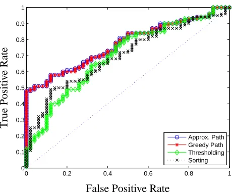
7.1 Artificial Data

We generate a matrix U of size 150 with uniformly distributed coefficients in[0,1]. We let v_∈R150 be a sparse vector with:

vi=







1 if i_≤50 1/(i₋50) if 50<i_≤100 0 otherwise.

0 0.2 0.4 0.6 0.8 1 0

0.1 0.2 0.3 0.4 0.5 0.6 0.7 0.8 0.9 1

Approx. Path Greedy Path Thresholding Sorting

PSfrag replacements

False Positive Rate

T

rue

Positi

v

e

Rate

Figure 1: ROC curves for sorting, thresholding, fully greedy solutions (Section 3.2) and approxi-mate greedy solutions (Section 3.3) forσ=2.

We then plot the variance versus cardinality tradeoff curves for various values of the signal-to-noise ratio. In Figure 2, We notice that the magnitude of the error (duality gap) decreases with the signal-to-noise ratio. Also, because of the structure of our problem, there is a kink in the variance at the (exact) cardinality 50 in each of these curves. Note that for each of these examples, the error (duality gap) is minimal precisely at the kink.

Next, we use the DSPCA algorithm of d’Aspremont et al. (2007b) to find better solutions where the greedy codes have failed to obtain globally optimal solutions. In d’Aspremont et al. (2007b), it was shown that an upper bound on (2) can be computed as:

φ(ρ)_≤ min |Ui j|≤ρ

λmax(Σ+U).

which is a convex problem in the matrix U_∈Sn. Note however that the cost of solving this relaxation for a single ρ is O(n4√_{log n) versus O(n}3_{) for a full path of approximate solutions. Also, the} results in d’Aspremont et al. (2007b) do not provide any hint on the value ofρ, but we can use the breakpoints coming from suboptimal points in the greedy search algorithms in Section 3.3 and the consistency intervals in Eq. (9). In Figure 2 we plot the variance versus cardinality tradeoff curve forσ=10. We plot greedy variances (solid line), dual upper bounds from Section 5.3 (dotted line) and upper bounds computed using DSPCA (dashed line).

7.2 Subset Selection

0 50 100 150 0

20 40 60 80 100 120

PSfrag replacements

Cardinality

V

ariance

10 20 30 40 50 60

5 10 15 20 25

PSfrag replacements

Cardinality

V

ariance

Figure 2: Left: variance versus cardinality tradeoff curves forσ=10 (bottom),σ=50 andσ=100 (top). We plot the variance (solid line) and the dual upper bounds from Section 5.3 (dotted line) for each target cardinality. Right: variance versus cardinality tradeoff curve for σ=10. We plot greedy variances (solid line), dual upper bounds from Section 5.3 (dotted line) and upper bounds computed using DSPCA (dashed line). Optimal points (for which the relative duality gap is less than 10−4) are in bold.

the optimality of solutions obtained from various algorithms such as the Lasso, forward greedy or backward greedy algorithms.

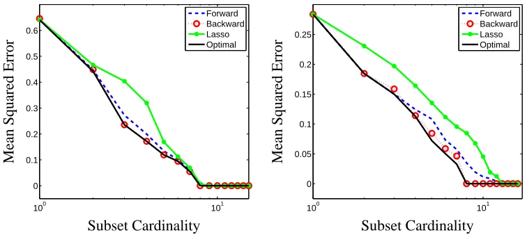
In Figure 3, we consider two pairs of randomly generated examples in dimension 16, one for which the lasso is provably consistent, one for which it isn’t. We perform 50 simulations with 1000 samples and varying noise and compute the average frequency of optimal subset selection for Lasso and greedy backward algorithm together with the frequency of provable optimality (i.e., where our method did ensure a posteriori that the point was optimal). We can see that the backward greedy algorithm exhibits good performance (even in the Lasso-inconsistent case) and that our sufficient optimality condition is satisfied as long as there is not too much noise. In Figure 4, we plot the average mean squared error versus cardinality, over 100 replications, using forward (dotted line) and backward (circles) selection, the Lasso (large dots) and exhaustive search (solid line). The plot on the left shows the results when the Lasso consistency condition is satisfied, while the plot on the right shows the mean squared errors when the consistency condition is not satisfied. The two sets of figures do show that the LASSO is consistent only when the consistency condition is satisfied, while the backward greedy algorithm finds the correct pattern if the noise is small enough (Couvreur and Bresler, 2000) even in the LASSO inconsistent case.

7.3 Sparse Recovery

Following the results of Section 6.2, we compute the upper and lower bounds on sparse eigenvalues produced using various algorithms. We study the following problem:

maximize xTΣx

subject to Card(x)_≤S

10−4 10−2 100 102 0

0.2 0.4 0.6 0.8 1

Greedy, prov. Greedy, ach. Lasso, ach.

PSfrag replacements

Noise Intensity

Probability

of

Optimality

10−4 10−2 100 102

0 0.2 0.4 0.6 0.8

1 Greedy, prov._{Greedy, ach.}

Lasso, ach.

PSfrag replacements

Noise Intensity

Probability

of

Optimality

Figure 3: Backward greedy algorithm and Lasso. We plot the probability of achieved (dotted line) and provable (solid line) optimality versus noise for greedy selection against Lasso (large dots), for the subset selection problem on a noisy sparse vector. Left: Lasso consistency condition satisfied. Right: consistency condition not satisfied.

100 101

0 0.1 0.2 0.3 0.4 0.5 0.6

Forward Backward Lasso Optimal

PSfrag replacements

Subset Cardinality

Mean

Squared

Error

100 101

0 0.05 0.1 0.15 0.2 0.25

Forward Backward Lasso Optimal

PSfrag replacements

Subset Cardinality

Mean

Squared

Error

1 2 3 4 5 6 7 8 2.5

3 3.5 4 4.5

Exhaustive App. Greedy Greedy SDP var. Dual Greedy Dual SDP Dual DSPCA

PSfrag replacements

Cardinality

Max.

Eigen

v

alue

2 4 6 8 10

1 1.2 1.4 1.6 1.8 2 2.2 2.4 2.6

Exhaustive App. Greedy Greedy SDP var. Dual Greedy Dual SDP Dual DSPCA

PSfrag replacements

Cardinality

Max.

Eigen

v

alue

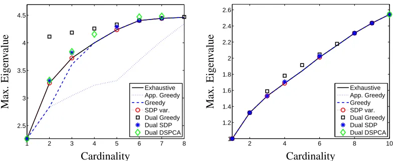
Figure 5: Upper and lower bound on sparse maximum eigenvalues. We plot the maximum sparse eigenvalue versus cardinality, obtained using exhaustive search (solid line), the approx-imate greedy (dotted line) and fully greedy (dashed line) algorithms. We also plot the upper bounds obtained by minimizing the gap of a rank one solution (squares), by solving the semidefinite relaxation explicitly (stars) and by solving the DSPCA dual (diamonds). Left: On a matrix FT_{F with F Gaussian. Right: On a sparse rank one plus noise matrix.}

where we pick F to be normally distributed and small enough so that computing sparse eigenvalues by exhaustive search is numerically feasible. We plot the maximum sparse eigenvalue versus cardi-nality, obtained using exhaustive search (solid line), the approximate greedy (dotted line) and fully greedy (dashed line) algorithms. We also plot the upper bounds obtained by minimizing the gap of a rank one solution (squares), by solving the semidefinite relaxation explicitly (stars) and by solving the DSPCA dual (diamonds). On the left, we use a matrixΣ=FTF with F Gaussian. On the right, Σ=uuT/_ku_k2+2V , where ui=1/i, i=1, . . . ,n and V is matrix with coefficients uniformly dis-tributed in[0,1]. Almost all algorithms are provably optimal in the noisy rank one case (as well as in many of the biological examples that follow), while Gaussian random matrices are harder. Note however, that the duality gap between the semidefinite relaxations and the optimal solution is very small in both cases, while our bounds based on greedy solutions are not as good. This means that solving the relaxations in (7) and d’Aspremont et al. (2007b) could provide very tight upper bounds on sparse eigenvalues of random matrices. However, solving these semidefinite programs for very large values of n remains a significant challenge.

7.4 Biological Data

Rank Rankgene GAN Description 3 8.6 J02854 Myosin regul.

6 18.9 T92451 Tropomyosin

7 31.5 T60155 Actin

8 25.1 H43887 Complement fact. D prec.

10 2.1 M63391 Human desmin

12 32.3 T47377 S-100P Prot.

Table 1: 6 genes (out of 4027) that were both in the top 20 sparse PCA genes and in the top 10 Rankgene genes.

0 50 100 150 200 250 300 350 400 450 500 0

0.5 1 1.5 2 2.5 3 3.5x 10

4

PSfrag replacements

Cardinality

V

ariance

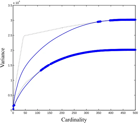
Figure 6: Variance (solid lines) versus cardinality tradeoff curve for two gene expression data sets, lymphoma (top) and colon cancer (bottom), together with dual upper bounds from Sec-tion 5.3 (dotted lines). Optimal points (for which the relative duality gap is less than 10−4) are in bold.

8. Conclusion

bounds. Having n matrix variables of dimension n, the problem is of course extremely large and finding numerical algorithms to directly optimize these relaxation bounds would be an important extension of this work.

Acknowledgments

The first author acknowledges support from NSF grant DMS-0625352, ONR grant number N00014-07-1-0150 and a gift from Google, Inc. We would like to thank Katya Scheinberg and the organizers of the Banff workshop on optimization and machine learning, where most of this paper was written.

Appendix A. Expansion of Eigenvalues

In this appendix, we consider various results on expansions of eigenvalues we use in order to derive sufficient conditions. The following proposition derives a second order expansion of the set of eigenvectors corresponding to a single eigenvalue.

Proposition 9 Let N _∈Sn. Let λ0 be an eigenvalue of N, with multiplicity r and eigenvectors U∈Rn×r(such that UTU=I). Let∆be a matrix in Sn. Ifk∆kF is small enough, the matrix N+∆ has exactly r (possibly equal) eigenvalues aroundλ0 and if we denote by(N+∆)λ0 the projection

of the matrix N+∆onto that eigensubspace, we have:

(N+∆)_λ0 = λ0UUT+UUT∆UUT+λ0UUT∆(λ0I−N)†+λ0(λ0I−N)†∆UUT

+UUT∆UUT∆(λ0I₋N)†+ (λ0I₋N)†∆UUT∆UUT+UUT∆(λ0I₋N)†UUT

+λ0UUT∆(λ0I₋N)†∆(λ0I₋N)†+λ0(λ0I₋N)†∆(λ0I₋N)†∆UUT

+λ0(λ0I−M)†∆UUT∆(λ0I−M)†+O(k∆k3F)

which implies the following expansion for the sum of the r eigenvalues in the neigborhood ofλ0: Tr(N+∆)_λ0 = rλ0+TrUT∆U+TrUT∆(λ0I−N)†∆U

+λ0Tr(λ0I−N)†∆UUT∆(λ0I−N)†+O(k∆k3F).

Proof We use the Cauchy residue formulation of projections on principal subspaces (Kato, 1966): given a symmetric matrix N, and a simple closed curve

C

ΠC(N) = 1

2iπ I

C

dλ λI₋N

is equal to the orthogonal projection onto the orthogonal sum of all eigensubspaces of N associated with eigenvalues in the interior of

C

i=1λiuiuTi , and the Cauchy residue formula (2i1π H

C λd−λλi =1 if λi is in the

interior int(

C

C

1 2iπ

I

C

dλ λI₋N =

n

∑

uiuTi × 1 2iπ

I

C

dλ λ−λi

=

∑

i,λi∈int(C)

See Rudin (1987) for an introduction to complex analysis and Cauchy residue formula. Moreover, we can obtain the restriction of N onto a specific sum of eigensubspaces as:

NΠC(N) = 1

2iπ I

C

Ndλ λI₋N =

1 2iπ

I

C

λdλ λI₋N.

From there we can easily compute expansions around a given N by using expansions of(λI−N)−1_. The proposition follows by considering a circle around λ0 that is small enough to exclude other eigenvalues of N, and applying several times the Cauchy residue formula.

We can now apply the previous proposition to our particular case:

Lemma 10 For any a _∈ Rn, ρ > 0 and B = aaT ₋ ρI, we consider the function F : X _7→Tr(X1/2_BX1/2₎

+ from Sn+ to R. let x∈Rn such thatkxk=1. Let Y 0. If xTBx>0, then

F((1₋t)xxT+tY) =xTBx+ t

xT_BxTr Bxx T_B(Y

−xxT) +O(t3/2),

while if xTBx<0, then

F((1₋t)xxT+tY) =Tr

Y1/2

B₋Bxx T_B

xT_Bx

Y1/2

+

+O(t3/2).

Proof We consider X(t) = (1₋t)xxT_{+tY . We have X(t) =U(t)U(t)}T_{with U(t) =}

(1₋t)1/2_x

t1/2Y1/2

,

which implies that the non zero eigenvalues of X(t)1/2_BX(t)1/2_{are the same as the non zero} eigen-values of U(t)T_{BU(t). We thus have}

F(X(t)) =Tr(M(t))+,

with

M(t) =

(1₋t)xT_{Bx t}1/2_(1−t)1/2_xT_BY1/2

t1/2(1₋t)1/2_yT_{Bx tY}1/2_BY1/2

=

xTBx 0 0 0

+t1/2

0 xTBY1/2 Y1/2Bx 0

+t

−xTBx 0 0 Y1/2BY1/2

+O(t3/2)

= M(0) +t1/2∆1+t∆2+O(t3/2).

The matrix M(0)has a single (and simple) non zero eigenvalue which is equal toλ0=xTBx with eigenvector U = (1,0)T_{. The only other eigenvalue of M(0) is zero, with multiplicity n.} Proposi-tion 9 can be applied to the two eigenvalues of M(0): there is one eigenvalue of M(t)around xTBx, while the n remaining ones are around zero. The eigenvalue close toλ0is equal to:

Tr(M(t))_λ0 = t TrU>∆2U+λ0+t TrUT∆1(λ0I−M(0))†∆1U

+λ0Tr(λ0I−M(0))†∆1UUT∆1(λ0I−M(0))†+O(t3/2)

= xTBx+ t

xT_BxTr Bxx T_B(Y

For the remaining eigenvalues, we get that the projected matrix on the eigensubspace of M(t) associated with eigenvalues around zero is equal to

(M(t))0 = t(I₋UUT)∆2(I₋UUT) +t(I₋UUT)∆1(₋M(0))†(I₋UUT) +O(t3/2)

=

0 0

0 tY1/2(B₋Bxx_xT_BxTB)Y1/2

,

which leads to a positive part equal to t+Tr

h

Y1/2(B₋BxxTB xT_Bx)Y1/2

i

+. When x

T_{Bx>0, then the}

ma-trix is negative definite (because B=aaT₋ρI), and thus the positive part is zero. By summing the two contributions, we obtain the desired result.

References

A. Alizadeh, M. Eisen, R. Davis, C. Ma, I. Lossos, and A. Rosenwald. Distinct types of diffuse large b-cell lymphoma identified by gene expression profiling. Nature, 403:503–511, 2000.

A. Alon, N. Barkai, D. A. Notterman, K. Gish, S. Ybarra, D. Mack, and A. J. Levine. Broad patterns of gene expression revealed by clustering analysis of tumor and normal colon tissues probed by oligonucleotide arrays. Cell Biology, 96:6745–6750, 1999.

A. Ben-Tal and A. Nemirovski. On tractable approximations of uncertain linear matrix inequalities affected by interval uncertainty. SIAM Journal on Optimization, 12(3):811–833, 2002.

S. Boyd and L. Vandenberghe. Convex Optimization. Cambridge University Press, 2004.

J. Cadima and I. T. Jolliffe. Loadings and correlations in the interpretation of principal components. Journal of Applied Statistics, 22:203–214, 1995.

E. J. Cand`es and T. Tao. Decoding by linear programming. Information Theory, IEEE Transactions on, 51(12):4203–4215, 2005.

C. Couvreur and Y. Bresler. On the optimality of the backward greedy algorithm for the subset selection problem. SIAM J. Matrix Anal. Appl., 21(3):797–808, 2000.

A. d’Aspremont, F. R. Bach, and L. El Ghaoui. Full regularization path for sparse principal compo-nent analysis. In Proceedings of the Twenty-fourth International Conference on Machine Learn-ing (ICML), 2007a.

A. d’Aspremont, L. El Ghaoui, M.I. Jordan, and G. R. G. Lanckriet. A direct formulation for sparse PCA using semidefinite programming. SIAM Review, 49(3):434–448, 2007b.

D. L. Donoho and J. Tanner. Sparse nonnegative solutions of underdetermined linear equations by linear programming. Proceedings of the National Academy of Sciences, 102(27):9446–9451, 2005.