Classes of Kernels for Machine Learning:
A Statistics Perspective
Marc G. Genton [email protected]
Department of Statistics
North Carolina State University Raleigh, NC 27695-8203, USA
Editors:Nello Cristianini, John Shawe-Taylor, Robert Williamson
Abstract
In this paper, we present classes of kernels for machine learning from a statistics perspective. Indeed, kernels are positive definite functions and thus also covariances. After discussing key properties of kernels, as well as a new formula to construct kernels, we present several important classes of kernels: anisotropic stationary kernels, isotropic stationary kernels, compactly supportedkernels, locally stationary kernels, nonstationary kernels, andsep-arable nonstationary kernels. Compactly supportedkernels andsepandsep-arable nonstationary kernels are of prime interest because they provide a computational reduction for kernel-based methods. We describe the spectral representation of the various classes of kernels and conclude with a discussion on the characterization of nonlinear maps that reduce non-stationary kernels to either stationarity or local stationarity.
Keywords: Anisotropic, Compactly Supported, Covariance, Isotropic, Locally Station-ary, NonstationStation-ary, Reducible, Separable, Stationary
1. Introduction
Recently, the use of kernels in learning systems has receivedconsiderable attention. The main reason is that kernels allow to map the data into a high dimensional feature space in order to increase the computational power of linear machines (see for example Vapnik, 1995, 1998, Cristianini andShawe-Taylor, 2000). Thus, it is a way of extending linear hypotheses to nonlinear ones, andthis step can be performedimplicitly. Support vector machines, kernel principal component analysis, kernel Gram-Schmidt, Bayes point machines, Gaussian processes, are just some of the algorithms that make crucial use of kernels for problems of classification, regression, density estimation, and clustering. In this paper, we present classes of kernels for machine learning from a statistics perspective. We discuss simple methods to design kernels in each of those classes and describe the algebra associated with kernels.
The kinds of kernel K we will be interestedin are such that for all examplesxand zin an input spaceX ⊂Rd:
K(x,z) =φ(x), φ(z),
important to be able to design new kernels. Clearly, from the symmetry of the inner product, a kernel must be symmetric:
K(x,z) =K(z,x),
andalso satisfy the Cauchy-Schwartz inequality:
K2(x,z)≤K(x,x)K(z,z).
However, this is not sufficient to guarantee the existence of a feature space. Mercer (1909) showedthat a necessary andsufficient condition for a symmetric function K(x,z) to be a kernel is that it be positive definite. This means that for any set of examplesx1, . . . ,xl and
any set of real numbersλ1, . . . , λl, the function K must satisfy: l
i=1
l
j=1
λiλjK(xi,xj)≥0. (1)
Symmetric positive definite functions are called covariances in the statistics literature. Hence kernels are essentially covariances, andwe propose a statistics perspective on the design of kernels. It is simple to create new kernels from existing kernels because positive definite functions have a pleasant algebra, and we list some of their main properties below. First, ifK1,K2 are two kernels, anda1,a2 are two positive real numbers, then:
K(x,z) =a1K1(x,z) +a2K2(x,z), (2)
is a kernel. This result implies that the family of kernels is a convex cone. The multiplication of two kernelsK1 and K2 yields a kernel:
K(x,z) =K1(x,z)K2(x,z). (3)
Properties (2) and(3) imply that any polynomial with positive coefficients, pol+(x) =
{n
i=1αixi|n∈N, α1, . . . , αn∈R+}, evaluatedat a kernelK1, yields a kernel:
K(x,z) =pol+(K1(x,z)). (4)
In particular, we have that:
K(x,z) = exp(K1(x,z)), (5) is a kernel by taking the limit of the series expansion of the exponential function. Next, if
g is a real-valuedfunction onX, then
K(x,z) =g(x)g(z), (6)
is a kernel. Ifψ is anRp-valuedfunction on X and K3 is a kernel onRp×Rp, then:
K(x,z) =K3(ψ(x), ψ(z)), (7)
is also a kernel. Finally, ifA is a positive definite matrix of size d×d, then:
is a kernel. The results (2)-(8) can easily be derived from (1), see also Cristianini and Shawe-Taylor (2000). The following property can be usedto construct kernels andseems not to be known in the machine learning literature. Let h be a real-valuedfunction on X, positive, with minimum at 0 (that is,h is a variance function). Then:
K(x,z) = 1 4
h(x+z)−h(x−z)
, (9)
is a kernel. The justification of (9) comes from the following identity for two random variables Y1 and Y2: Covariance(Y1,Y2)=[Variance(Y1 +Y2)−Variance(Y1 −Y2)]/4. For instance, consider the functionh(x) =xTx. From (9), we obtain the kernel:
K(x,z) = 1 4
(x+z)T(x+z)−(x−z)T(x−z)
=xTz.
The remainder of the paper is set up as follows. In Section 2, 3, and 4, we discuss respectively the class of stationary, locally stationary, andnonstationary kernels. Of par-ticular interest are the classes of compactly supportedkernels andseparable nonstationary kernels because they reduce the computational burden of kernel-based methods. For each class of kernels, we present their spectral representation andshow how it can be usedto design many new kernels. Section 5 addresses the reducibility of nonstationary kernels to stationarity or local stationarity, andwe conclude the paper in Section 6.
2. Stationary Kernels
A stationary kernel is one which is translation invariant:
K(x,z) =KS(x−z),
that is, it depends only on the lag vector separating the two examplesx and z, but not on the examples themselves. Such a kernel is sometimes referredto as anisotropic stationary kernel, in order to emphasize the dependence on both the direction and the length of the lag vector. The assumption of stationarity has been extensively usedin time series (see for example Brockwell andDavis, 1991) andspatial statistics (see for example Cressie, 1993) because it allows for inference on K basedon all pairs of examples separatedby the same lag vector. Many stationary kernels can be constructedfrom their spectral representation derived by Bochner (1955). He proved that a stationary kernelKS(x−z) is positive definite inRd if andonly if it has the form:
KS(x−z) =
Rd
cosωT(x−z)F(dω), (10)
When a stationary kernel depends only on the norm of the lag vector between two examples, andnot on the direction, then the kernel is saidto be isotropic (or homogeneous), andis thus only a function of distance:
K(x,z) =KI(x−z).
The spectral representation of isotropic stationary kernels has been derived from Bochner’s theorem (Bochner, 1955) by Yaglom (1957):
KI(x−z) =
∞
0
Ωdωx−zF(dω), (11)
where
Ωd(x) =
2
x
(d−2)/2 Γ
d
2 J(d−2)/2(x),
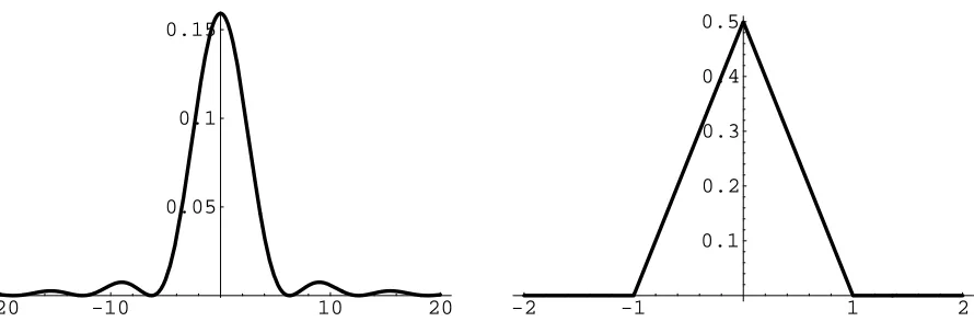
form a basis for functions in Rd. Here F is any nondecreasing bounded function, Γ(d/2) is the gamma function, and Jv is the Bessel function of the first kindof order v. Some familiar examples of Ωd are Ω1(x) = cos(x), Ω2(x) = J0(x), andΩ3(x) = sin(x)/x. Here again, by choosing a nondecreasing bounded functionF (or its derivativef), we can derive the corresponding kernel from (11). For instance in R1, with the spectral density f(ω) = (1−cos(ω))/(πω2), we derive the triangular kernel:
KI(x−z) =
∞
0
cos(ω|x−z|)1−cos(ω)
πω2 dω
= 1
2(1− |x−z|) +,
where (x)+ = max(x,0) (see Figure 1). Note that an isotropic stationary kernel obtained with Ωd is positive definite in Rd andin lower dimensions, but not necessarily in higher dimensions. For example, the kernelKI(x−z) = (1− |x−z|)+/2 is positive definite inR1 but not in R2, see Cressie (1993, p.84) for a counterexample. It is interesting to remark from (11) that an isotropic stationary kernel has a lower bound(Stein, 1999):
KI(x−z)/KI(0)≥ inf
x≥0Ωd(x), thus yielding:
KI(x−z)/KI(0) ≥ −1 in R1
KI(x−z)/KI(0) ≥ −0.403 inR2
KI(x−z)/KI(0) ≥ −0.218 inR3
KI(x−z)/KI(0) ≥ 0 in R∞.
-20 -10 10 20 0.05
0.1 0.15
-2 -1 1 2
0.1 0.2 0.3 0.4 0.5
Figure 1: The spectral density f(ω) = (1 −cos(ω))/(πω2) (left) andits corresponding isotropic stationary kernelKI(x−z) = (1− |x−z|)+/2 (right).
(1938) provedthat if βd is the class of positive definite functions of the form given by Bochner (1955), then the classes for alldhave the property:
β1 ⊃β2⊃ · · · ⊃βd⊃ · · · ⊃β∞,
so that asdis increased, the space of available functions is reduced. Only functions with the basis exp(−x2) are containedin all the classes. The positive definite requirement imposes a smoothness condition on the basis as the dimensiondis increased. Several criteria to check the positive definiteness of stationary kernels can be found in Christakos (1984). Further isotropic stationary kernels defined with non-Euclidean norms have recently been discussed by Christakos andPapanicolaou (2000).
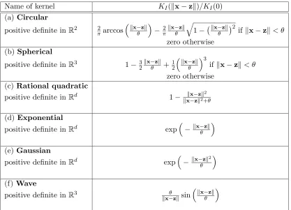
From the spectral representation (11), we can construct many isotropic stationary ker-nels. Some of the most commonly usedare depictedin Figure 2. They are definedby the equations listedin Table 1, whereθ >0 is a parameter. As an illustration, the exponential kernel (d) is obtained from the spectral representation (11) with the spectral density:
f(ω) = π 1
θ +πθω2
,
whereas the Gaussian kernel (e) is obtainedwith the spectral density:
f(ω) =
√
θ
2√π exp
−θω2
4 .
Note also that the circular andspherical kernels have compact support. They have a linear behavior at the origin, which is also true for the exponential kernel. The rational quadratic, Gaussian, and wave kernels have a parabolic behavior at the origin. This indicates a different degree of smoothness. Finally, the Mat´ern kernel (Mat´ern, 1960) has recently received considerable attention, because it allows to control the smoothness with a parameter ν. The Mat´ern kernel is defined by:
KI(x−z)/KI(0) = 1 2ν−1Γ(ν)
2√νx−z
θ
ν
Hν
2√νx−z
-4 -2 2 4 0.2
0.4 0.6 0.8 1
-4 -2 2 4
0.2 0.4 0.6 0.8 1
(a) (b)
-4 -2 2 4
0.2 0.4 0.6 0.8 1
-4 -2 2 4
0.2 0.4 0.6 0.8 1
(c) (d)
-4 -2 2 4
0.2 0.4 0.6 0.8 1
-4 -2 2 4
-0.2 0.2 0.4 0.6 0.8 1
(e) (f)
Figure 2: Some isotropic stationary kernels: (a) circular; (b) spherical; (c) rational quadratic; (d) exponential; (e) Gaussian; (f) wave.
Name of kernel KI(x−z)/KI(0) (a)Circular
positive definite in R2 π2 arccos
x−z
θ
− 2
π
x−z
θ
1−x−θz2 ifx−z< θ
zero otherwise (b)Spherical
positive definite in R3 1−32x−θz +12
x−z
θ
3
ifx−z< θ
zero otherwise (c) Rational quadratic
positive definite in Rd 1−x−x−zz2+2θ (d)Exponential
positive definite in Rd exp
−x−θz
(e) Gaussian
positive definite in Rd exp
−x−θz2
(f) Wave
positive definite in R3 θ
x−zsin
x−z
θ
Table 1: Some commonly usedisotropic stationary kernels.
to the Gaussian kernel for ν → ∞. Therefore, the Mat´ern kernel includes a large class of kernels andwill prove very useful for applications because of this flexibility.
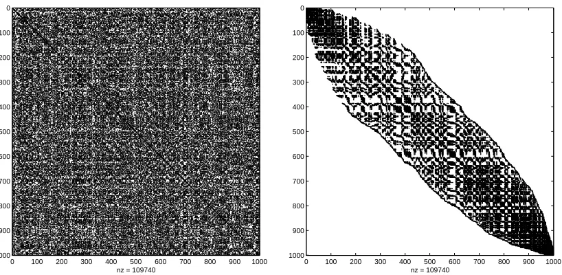
Compactly supportedkernels are kernels that vanish whenever the distance between two examples x and z is larger than a certain cut-off distance, often called the range. For instance, the spherical kernel (b) is a compactly supportedkernel since KI(x−z) = 0 when x−z ≥ θ. This might prove a crucial advantage for certain applications dealing with massive data sets, because the corresponding Gram matrix G, whose ij-th element is Gij = K(xi,xj), will be sparse. Then, linear systems involving the matrix G can be
0 100 200 300 400 500 600 700 800 900 1000 0
100
200
300
400
500
600
700
800
900
1000
nz = 109740
0 100 200 300 400 500 600 700 800 900 1000 0
100
200
300
400
500
600
700
800
900
1000
nz = 109740
Figure 3: The Gram matrix for 1,000 examples uniformly distributed in the unit square, basedon a spherical kernel with rangeθ= 0.2: initial (left panel); after reordering (right panel).
spherical andthe circular kernels wouldbe the only compactly supportedkernels available, this technique wouldbe limited. Fortunately, large classes of compactly supportedkernels can be constructed, see for example Gneiting (2002a) and references therein. A compactly supportedkernel of Mat´ern type can be obtainedby multiplying the kernel (12) by the kernel:
max
1−x−z ˜
θ
˜
ν
,0
,
where ˜θ >0 and˜ν ≥(d+ 1)/2, in order to insure positive definiteness. This product is a kernel by the property (3). Beware that it is not possible to simply “cut-off” a kernel in order to obtain a compactly supported one, because the result will not be positive definite in general.
3. Locally Stationary Kernels
A simple departure from the stationary kernels discussed in the previous section is provided by locally stationary kernels (Silverman, 1957, 1959):
K(x,z) =K1
x+z
2
K2(x−z), (13)
constant, we further impose that K2(0) = 1. The variable (x+z)/2 has been chosen because of its suggestive meaning of the average or centroidof the examplesx andz. The variance is determined by:
K(x,x) =K1(x)K2(0) =K1(x), (14)
thus justifying the name of power schedule forK1(x), which describes the global structure. On the other hand,K2(x−z) is invariant under shifts and thus describes the local structure. It can be obtainedby considering:
K(x/2,−x/2) =K1(0)K2(x). (15)
Equations (14) and(15) imply that the kernelK(x,z) defined by (13) is completely deter-minedby its values on the diagonal x=zandantidiagonalx=−z, for:
K(x,z) = K((x+z)/2,(x+z)/2)K((x−z)/2,−(x−z)/2)
K(0,0) . (16)
Thus, we see thatK1is invariant with respect to shifts parallel to the antidiagonal, whereas
K2 is invariant with respect to shifts parallel to the diagonal. These properties allow to findmoment estimators of bothK1 andK2 from a single realization of data, although the kernel is not stationary.
We already mentioned that stationary kernels are locally stationary. Another special class of locally stationary kernels is defined by kernels of the form:
K(x,z) =K1(x+z), (17)
the so-calledexponentially convex kernels (Lo`eve, 1946, 1948). From (16), we see immedi-ately that K1(x+z)≥0. Actually, as notedby Lo`eve, any two-sided Laplace transform of a nonnegative function is an exponentially convex kernel. A large class of locally stationary kernels can therefore be constructedby multiplying an exponentially convex kernel by a stationary kernel, since the product of two kernels is a kernel by the property (3). However, the following example is a locally stationary kernel in R1 which is not the product of two kernels:
exp
−a(x2+z2)
= exp
−2a((x+z)/2)2
exp
−a(x−z)2/2
, a >0, (18)
since the first factor in the right side is a positive function without being a kernel, and the secondfactor is a kernel. Finally, with the positive definite Delta kernelδ(x−z), which is equal to 1 if x=zand0 otherwise, the product:
K(x,z) =K1 x+z
2
δ(x−z),
is a locally stationary kernel, often calleda locally stationary white noise.
The spectral representation of locally stationary kernels has remarkable properties. In-deed, it can be written as (Silverman, 1957):
K(x,z) =
Rd
Rd
cosωT1x−ωT2z
f1
ω1+ω2
2
i.e. the spectral densityf1
ω1+ω2 2
f2(ω1−ω2) is also a locally stationary kernel, and:
K1(u) =
Rd
cos(ωTu)f2(ω)dω,
K2(v) =
Rd
cos(ωTv)f1(ω)dω,
i.e. K1, f2 and K2, f1 are Fourier transform pairs. For instance, to the locally stationary kernel (18) corresponds the spectral density:
f1 ω
1+ω2 2
f2(ω1−ω2) = 1 4πaexp
− 1
2a((ω1+ω2)/2)
2exp− 1
8a(ω1−ω2)
2/2, which is immediately seen to be locally stationary since, except for a positive factor, it is of the form (18), with a replacedby 1/(4a). Thus, we can design many locally stationary kernels with the help of their spectral representation. In particular, we can obtain a very rich family of locally stationary kernels by multiplying a Mat´ern kernel (12) by an exponentially convex kernel (17). The resulting product is still a kernel by the property (3).
4. Nonstationary Kernels
The most general class of kernels is the one of nonstationary kernels, which depend explicitly on the two examplesx and z:
K(x,z).
For example, the polynomial kernel of degree p:
K(x,z) = (xTz)p,
is a nonstationary kernel. The spectral representation of nonstationary kernels is very general. A nonstationary kernel K(x,z) is positive definite in Rd if andonly if it has the form (Yaglom, 1987):
K(x,z) =
Rd
Rd
cosωT1x−ωT2z
F(dω1, dω2), (19)
where F is a positive bounded symmetric measure. When the function F(ω1,ω2) is con-centratedon the diagonalω1 =ω2, then (19) reduces to the spectral representation (10) of stationary kernels. Here again, many nonstationary kernels can be constructedwith (19). Of interest are nonstationary kernels obtainedfrom (19) withω1=ω2 but with a spectral density that is not integrable in a neighborhoodaroundthe origin. Such kernels are referred to as generalizedkernels (Matheron, 1973). For instance, the Brownian motion generalized kernel corresponds to a spectral densityf(ω) = 1/ω2 (Mandelbrot and Van Ness, 1968).
A particular family of nonstationary kernels is the one of separable nonstationary kernels:
K(x,z) =K1(x)K2(z),
kernels possess the property that their Gram matrix G, whose ij-th element is Gij =
K(xi,xj), can be written as a tensor product (also called Kronecker product, see Graham,
1981) of two vectors defined by K1 and K2 respectively. This is especially useful to reduce computational burden when dealing with massive data sets. For instance, consider a set ofl
examplesx1, . . . ,xl. The memory requirements fot the computation of the Gram matrix is
then reduced froml2to 2lsince it suffices to evaluate the vectorsa= (K1(x1), . . . , K1(xl))T and b = (K2(x1), . . . , K2(xl))T. We then haveG=abT. Such a computational reduction
can be of crucial importance for certain applications involving very large training sets.
5. Reducible Kernels
In this section, we discuss the characterization of nonlinear maps that reduce nonstationary kernels to either stationarity or local stationarity. The main idea is to find a new feature space where stationarity (see Sampson andGuttorp, 1992) or local stationarity (see Genton andPerrin, 2001) can be achieved. We say that a nonstationary kernelK(x,z) is stationary reducible if there exist a bijective deformation Φsuch that:
K(x,z) =KS∗(Φ(x)−Φ(z)), (20)
whereKS∗ is a stationary kernel. For example inR2, the nonstationary kernel defined by:
K(x,z) =x+z − z−x
2xz , (21)
is stationary reducible with the deformation:
Φ(x1, x2) =
lnx2 1+x22
,arctan(x2/x1) T
,
yielding the stationary kernel:
KS∗(u1, u2) = cosh(u1/2)−
(cosh(u1/2)−cos(u2))/2. (22) Effectively, it is straightforwardto check with some algebra that (22) evaluatedat:
Φ(x)−Φ(z) =
ln
x
z ,arctan(x2/x1)−arctan(z2/z1)
T
,
yields the kernel (21). Perrin and Senoussi (1999, 2000) characterize such deformations
Φ. Specifically, if Φ andits inverse are differentiable in Rd, and K(x,z) is continuously differentiable forx=y, thenK satisfies (20) if andonly if:
DxK(x,z)QΦ−1(x) +DzK(x,z)Q−Φ1(z) =0, x=y, (23) whereQΦis the Jacobian ofΦandDxdenotes the partial derivatives operator with respect tox. It can easily be checkedthat the kernel (21) satisfies the above equation (23). Unfor-tunately, not all nonstationary kernels can be reduced to stationarity through a deformation
Φ. Consider for instance the kernel inR1:
which is positive definite as can be seen from (6). It is obvious that K(x, z) d oes not satisfy Equation (23) andthus is not stationary reducible. This is the motivation of Genton andPerrin (2001) to extendthe model (20) to locally stationary kernels. We say that a nonstationary kernelK is locally stationary reducible if there exists a bijective deformation
Φsuch that:
K(x,z) =K1
Φ(x) +Φ(z)
2
K2
Φ(x)−Φ(z), (25)
where K1 is a nonnegative function and K2 is a stationary kernel. Note that if K1 is a positive constant, then Equation (25) reduces to the model (20). Genton and Perrin (2001) characterize such transformations Φ. For instance, the nonstationary kernel (24) can be reduced to a locally stationary kernel with the transformation:
Φ(x) = x 3 3 −
1
3, (26)
yielding:
K1(u) = exp
−18u2−12u (27)
K2(v) = exp
−9
2v
2 . (28)
Here again, it can easily be checkedfrom (27), (28), and(26) that:
K1
Φ(x) +Φ(z)
2
K2
Φ(x)−Φ(z)= exp(2−x6−z6).
Of course, it is possible to construct nonstationary kernels that are neither stationary re-ducible nor locally stationary rere-ducible. Actually, the familiar class of polynomial kernels of degree p,K(x,z) = (xTz)p, cannot be reduced to stationarity or local stationarity with
a bijective transformationΦ. Further research is needed to characterize such kernels.
6. Conclusion
Acknowledgments
I wouldlike to acknowledge support for this project from U.S. Army TACOM Research, Development andEngineering Center under the auspices of the U.S. Army Research Office Scientific Services Program administered by Battelle (Delivery Order 634, Contract No. DAAH04-96-C-0086, TCN 00-131). I wouldlike to thank DavidGorsich from U.S. Army TACOM, Olivier Perrin, as well as the Editors and two anonymous reviewers, for their comments that improvedthe manuscript.
References
N. Aronszajn. Theory of reproducing kernels. Trans. American Mathematical Soc., 68: 337–404, 1950.
S. Bochner. Harmonic Analysis and the Theory of Probability. University of California Press, Los Angeles, California, 1955.
P. J. Brockwell andR. A. Davis. Time Series: Theory and Methods. Springer, New York, 1991.
G. Christakos. On the problem of permissible covariance andvariogram models. Water Resources Research, 20(2):251–265, 1984.
G. Christakos. Modern Spatiotemporal Geostatistics. OxfordUniversity Press, New York, 2000.
G. Christakos and V. Papanicolaou. Norm-dependent covariance permissibility of weakly homogeneous spatial random fields and its consequences in spatial statistics. Stochastic Environmental Research and Risk assessment, 14(6):471–478, 2000.
N. Cressie. Statistics for Spatial Data. John Wiley & Sons, New York, 1993.
N. Cressie andH.-C. Huang. Classes of nonseparable, spatio-temporal stationary covariance functions. Journal of the American Statistical Association, 94(448):1330–1340, 1999.
N. Cristianini andJ. Shawe-Taylor. An Introduction to Support Vector Machines and other Kernel-based Learning Methods. Cambridge University Press, Cambridge, 2000.
M. G. Genton and O. Perrin. On a time deformation reducing nonstationary stochastic processes to local stationarity. Technical Report NCSU, 2001.
J. R. Gilbert, C. Moler, andR. Schreiber. Sparse matrices in MATLAB: design andimple-mentation. SIAM Journal on Matrix Analysis, 13(1):333–356, 1992.
T. Gneiting. Compactly supportedcorrelation functions. Journal of Multivariate Analysis, to appear, 2002a.
A. Graham. Kronecker Products and Matrix Calculus: with Applications. Ellis Horwood Limited, New York, 1981.
M. Lo`eve. Fonctions al´eatoires `a d ´ecomposition orthogonale exponentielle. La Revue Sci-entifique, 84:159–162, 1946.
M. Lo`eve. Fonctions al´eatoires du second ordre. In: Processus Stochastiques et Mouvement Brownien (P. L´evy), Gauthier-Villars, Paris, 1948.
B. B. Mandelbrot and J. W. Van Ness. Fractional brownian motions, fractional noises and applications. SIAM Review, 10:422–437, 1968.
B. Mat´ern. Spatial Variation. Springer, New York, 1960.
G. Matheron. The intrinsic random functions and their applications. J. Appl. Probab., 5: 439–468, 1973.
J. Mercer. Functions of positive andnegative type andtheir connection with the theory of integral equations. Philos. Trans. Roy. Soc. London, A 209:415–446, 1909.
O. Perrin andR. Senoussi. Reducing non-stationary stochastic processes to stationarity by a time deformation. Statistics and Probability Letters, 43(4):393–397, 1999.
O. Perrin and R. Senoussi. Reducing non-stationary random fields to stationarity and isotropy using a space deformation. Statistics and Probability Letters, 48(1):23–32, 2000.
P. D. Sampson andP. Guttorp. Nonparametric estimation of nonstationary spatial covari-ance structure. Journal of the American Statistical Association, 87(417):108–119, 1992.
I. J. Schoenberg. Metric spaces andcompletely monotone functions.Annals of Mathematics, 39(3):811–841, 1938.
R. A. Silverman. Locally stationary random processes. IRE Transactions Information Theory, 3:182–187, 1957.
R. A. Silverman. A matching theorem for locally stationary random processes. Communi-cations on Pure and Applied Mathematics, 12:373–383, 1959.
M. Stein. Interpolation of Spatial Data: Some Theory for Kriging. Springer, New York, 1999.
V. Vapnik. The Nature of Statistical Learning Theory. Springer, New York, 1995.
V. Vapnik. Statistical Learning Theory. Wiley, New York, 1998.
A. M. Yaglom. Some classes of random fields in n-dimensional space, related to stationary random processes. Theory of Probability and its Applications, 2:273–320, 1957.