* Corresponding author. Tel: +1-801-863-8858 E-mail: [email protected] (M. Hamidi) © 2014 Growing Science Ltd. All rights reserved. doi: 10.5267/j.ijiec.2013.09.008
International Journal of Industrial Engineering Computations 5 (2014) 87–100
Contents lists available at GrowingScience
International Journal of Industrial Engineering Computations
homepage: www.GrowingScience.com/ijiec
A heuristic algorithm for a multi-product four-layer capacitated location-routing problem
Mohsen Hamidia*, Kambiz Farahmandb, S. Reza Sajjadic and Kendall E. Nygardd
a
Finance and Economics Department, Woodbury School of Business, Utah Valley University, USA b
Department of Industrial and Manufacturing Engineering, North Dakota State University, NDSU Department, 2485, P.O. Box 6050, Fargo, North Dakota 58108-6050, USA
c
TransSolutions, LLC, 14600 Trinity Blvd., Suite 200, Fort Worth, TX 76155, USA d
Department of Computer Science, North Dakota State University, IACC 258, 2740, P.O. Box 6050, Fargo, ND 58108-6050, USA C H R O N I C L E A B S T R A C T
Article history: Received July 2 2013
Received in revised format September 7 2013
Accepted September 27 2013 Available online
September 27 2013
The purpose of this study is to solve a complex multi-product four-layer capacitated location-routing problem (LRP) in which two specific constraints are taken into account: 1) plants have limited production capacity, and 2) central depots have limited capacity for storing and transshipping products. The LRP represents a multi-product four-layer distribution network that consists of plants, central depots, regional depots, and customers. A heuristic algorithm is developed to solve the four-layer LRP. The heuristic uses GRASP (Greedy Randomized Adaptive Search Procedure) and two probabilistic tabu search strategies of intensification and diversification to tackle the problem. Results show that the heuristic solves the problem effectively.
© 2014 Growing Science Ltd. All rights reserved
Keywords:
Location-Routing Problem (LRP) Distribution Network
GRASP (Greedy Randomized Adaptive Search Procedure) Tabu Search
1. Introduction
(Min et al., 1998). Some LRP applications are food and drink distribution, newspaper distribution, parcel delivery, and waste collection (Nagy & Salhi, 2007). The LRP is one of the combinatorial optimization problems (Nagy & Salhi, 2007). LRP models include too many variables and constraints to be solved in a short amount of time by exact methods (Laporte, 1988). The LRP is an NP-hard, Non-deterministic Polynomial-time hard, problem, and exact methods can only solve small problems in a reasonable amount of time (Nagy & Salhi, 2007). The useful methods to solve larger LRPs have been heuristics (Ambrosino & Scutella, 2005).
2. Literature Review
The majority of studied LRP models are two-layer LRPs in which the distribution network consists of two layers of depots and customers (Ambrosino & Scutella, 2005). Two-layer LRPs solve three problems (Hamidi et al., 2011, 2012a, 2012b): 1) location problem: given a series of candidate locations, how many depots should exist and where should they be placed?, 2) allocation problem: which customers should be assigned to which depot?, and 3) routing problem: how many tours are needed for each depot, which customers should be served on each tour, and what is the order of customers on each tour?. In this section some of the two-layer LRPs are reviewed. Wu et al. (2002) used simulated annealing and tabu search to solve the location-allocation problem and the vehicle routing problem sequentially and iteratively. Prins et al. (2006) applied GRASP followed by a path
relinking procedure to tackle the LRP. Barreto et al. (2007) presented a cluster analysis based
sequential heuristic. Marinakis and Marinaki (2008) developed a bi-level formulation that decomposes the problem to a capacitated facility location problem and a vehicle routing problem. They used genetic algorithm, GRASP, and neighborhood search techniques in their heuristic. Duhamel et al. (2010) introduced a heuristic that is a GRASP hybridized with an evolutionary local search. Yu et al. (2010) used simulated annealing to solve the LRP.
Lei (2009) discussed a three-layer LRP. The decisions are: 1) the locations of distribution centers (DC’s), 2) identifying the big clients to be included in the first level routing (the routing between plants, DC’s, and big clients), 3) the first-level routing, and 4) the second-level routing between DC’s and other clients not included in the first-level routing. The authors used a genetic algorithm heuristic to solve the problem. Ambrosino et al. (2009) studied a three-layer LRP consisting of one central depot, regional depots, and customers. In the network, customers are partitioned into regions. One regional depot should be selected in each region. The central depot provides general products, and the regional depots provide regional products. In each region each tour must include both the central depot and the selected regional depot. The authors modeled the LRP as a mixed-integer linear programming model and introduced a heuristic that uses clustering and neighborhood search techniques. The heuristic is useful only for small and medium-size problems. The computational time is very large for large problems. Lee et al. (2010) discussed a four-layer LRP in which only one product is distributed. The network consists of suppliers, manufacturers, distribution centers (DC), and customers. The decisions are: 1) location, locating manufacturers and DCs; 2) allocation, allocating suppliers to manufacturers and allocating customers to DCs; 3) routing, routing between manufacturers and suppliers starting from manufacturers and routing between DCs and customers starting from DCs; and 4) transportation, transporting products from manufacturers to DCs. The comprehensive surveys on the LRP can be found in Balakrishnan et al. (1987), Laporte (1988), Min et al. (1998), and Nagy and Salhi (2007).
3. The Multi-Product Four-Layer Distribution Network
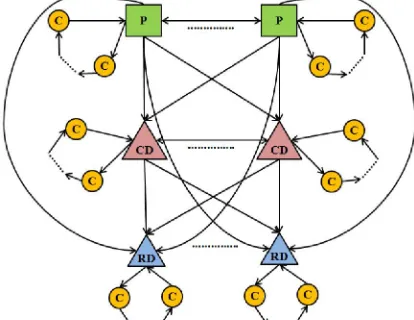
The LRP studied in this work is a complex multi-product four-layer capacitated LRP. This LRP is an extension of the LRP that we discussed in Hamidi et al. (2012b). As we described in Hamidi et al. (2011, 2012a, 2012b), the four-layer LRP represents a distribution network consisting of plants (P), central depots (CD), regional depots (RD), and customers (C). This distribution network is depicted in Fig. 1. General characteristics of this distribution network are as follows (Hamidi et al., 2012b):
Unlike Ambrosino and Scutella’s (2005) study, this distribution network has multiple plants, and multiple products are distributed in the network. Plants produce different types of products and send them to customers directly or through depots. Direct shipment between facilities (Plants, CDs, RDs) is allowed if the distance between the facilities is less than a maximum direct shipment distance. CDs can be used to transship products to other depots.
In Ambrosino and Scutella’s (2005) and Lee et al.’s (2010) studies customers can be served only by depots. But in this distribution network customers can be directly served by depots and plants. Multiple customers can be served in one tour. In Fig. 1 only one tour is shown for each facility, but several tours can be originated from the facility. Every customer is included in only one tour. The tour length is limited.
In the LRP discussed in this work, we take into account two specific constraints and add them to the LRP that we studied in Hamidi et al. (2012b). The constraints are as follows:
1) Plants have limited production capacity. In the scenario that we discussed in Hamidi et al. (2012b), each plant produces all types of products, and the production capacity for each product is unlimited (very large). But in the LRP presented in this paper each plant does not necessarily produce all types of products and has a certain production capacity for each product.
2) Central depots have limited capacity for storing and transshipping products. In Hamidi et al. (2012b) it is assumed that to transship products, CDs have unlimited storage capacity.
In this new scenario, each plant may have to send products to other plants directly or through CDs. Also, each facility may have to receive products from multiple facilities. We developed and presented the formulation of this LRP as a mixed integer programming model in Hamidi et al. (2011, 2012a). The decisions of the LRP are (Hamidi et al., 2011, 2012a): 1) location, locating CDs and RDs; 2) allocation, allocating customers to facilities; 3) transshipment between facilities; and 4) routing between facilities and customers. Since large LRPs cannot be solved in a reasonable amount of time by using exact algorithms, we developed a heuristic that is capable of solving large problems. The heuristic is presented in the following section.
4. The Heuristic Algorithm
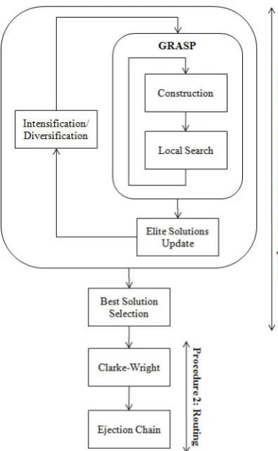
The heuristic developed for this LRP uses the same structure of the heuristic that we had developed for the LRP in Hamidi et al. (2012b) but the content of the heuristic is different. The heuristic structure is shown in Fig. 2.
We used GRASP (Greedy Randomized Adaptive Search Procedure) and two tabu search strategies of intensification and diversification in the first procedure of the heuristic. GRASP has two phases of construction and local search (Feo & Resende, 1995). The construction phase creates a greedy randomized solution, and the local search improves the solution by searching the neighborhood of the solution (Resende & Ribeiro, 2003). The intensification strategy in tabu search tries to generate solutions that are similar to high quality solutions, and the diversification strategy tries to generate solutions that are different from the generated solutions and search the areas of the solution space that have not been searched (Glover & Laguna, 1997). The core and the most important part of the heuristic is the construction phase of GRASP. In the construction phase, we developed a 7-step GRASP for the LRP presented in Hamidi et al. (2012b), whereas for the LRP presented in this paper a 13-step GRASP has been developed to consider the two additional constraints mentioned in the previous section. Also, in the local search phase the content of the transshipment path swap and the way it works is different from the transshipment path swap presented in Hamidi et al. (2012b).
Procedure 1: Location-Allocation-Transshipment
This procedure selects depots, assigns customers to facilities, and builds transshipment paths. In each round of the GRASP, n solutions are generated by the construction phase and improved by the local search phase. The steps of these two phases are as follows. In these steps, a facility is a plant, a CD, or an RD. Also, a depot is a CD or an RD. As shown in Fig. 2, after each round of the GRSAP, the list of elite solutions, best solutions found so far, is updated.
Construction Phase
Step 1. For each plant, allocate the customers whose distances from the plant are less than or equal to the coverage radius. The coverage radius is the maximum desirable distance of a customer from a facility to which the customer can be allocated. From the practical point of view, it is not desirable to assign distant customers to the facility because multiple customers are to be served in each tour and the tour length is limited. So, this radius can be a fraction (less than ½) of the maximum tour length, e.g. one fourth of the maximum tour length, to make sure that multiple customers are served in one tour.
Step 2. For each plant, calculate the demand of the plant for each product; the demand of the plant is the total demand of the customers assigned to the plant. The minimum of the production capacity of the plant for the product and the demand of the plant is assigned to the plant. If there is unsatisfied demand for the plant, go to Step 3 (the plant is called the facility), otherwise go to Step 8.
Step 3. If there is a plant whose distance from the facility is less than the maximum direct shipment distance, the minimum of the remaining production capacity of the plant for the product and the unsatisfied demand of the facility is assigned to the plant, and a transshipment path is constructed from the plant to the facility. If there is unsatisfied demand for the facility, do Step 4 and Step 5 until the demand is satisfied.
Step 4. Select the nearest plant to the facility that has a remaining production capacity for the product more than zero. The minimum of the remaining production capacity of the plant for the product and the unsatisfied demand is called XX.
Step 5. Among plants and open CDs with the following conditions, find the nearest one to the selected plant (called facility B).
Their distances from the facility are less than the maximum direct shipment distance. Their remaining throughput capacity is more than zero.
If no such a facility is found, among closed CDs whose distances from the facility are less than the maximum direct shipment distance, find the nearest one to the selected plant (called facility B) and open it. The minimum of XX and the remaining throughput capacity of facility B for the product is called XX1. Construct a transshipment path from facility B to the facility. Increase the unsatisfied demand of facility B by XX1. Reduce XX by XX1. Reduce the unsatisfied demand of the facility by XX1. If XX is not zero, restart Step 5. If XX is zero and there is still unsatisfied demand, go to Step 4.
Step 6. For each opened CD with unsatisfied demand, go to Step 3 to construct the transshipment paths.
Step 7. For each open CD, do the following:
Assign the near unassigned customers to the depot until the remaining capacity of the depot is less than the customer’s demand or the distance between the depot and the customer is more than the coverage radius; sort the unassigned customers based on their distances to the depot and start from the nearest customer.
For each product, calculate the demand of the facility. Go to Step 3 to construct the transshipment paths.
Step 8. Create the main list. Add all of the plants and already opened CDs to the main list; the main list includes all plants and open CDs some of which will be added to the list in following steps. Select the first facility in the main list.
Step 9. Create the restricted candidate list (RCL) for the selected facility. The RCL for the facility is the list of depots with the following characteristics:
The depot is unopened.
The nearest customer to the depot has not been assigned to any facility.
The depot can directly be connected to the selected facility; its distance to the facility is less than or equal to the maximum direct shipment distance.
If the selected facility is a CD, only depots that cannot directly be connected to any plant can be in the RCL.
Step 10. From the RCL of the selected facility, randomly select a depot and do the following: Open the depot.
If the depot is a CD, add it to the end of the main list.
Assign the near unassigned customers to the depot until the remaining capacity of the depot is less than the customer’s demand or the distance between the depot and the customer is more than the coverage radius; sort the unassigned customers based on their distances to the depot and start from the nearest customer.
Do Steps 3 to 7 to construct the transshipment paths.
Step 11. If all customers are assigned, finish the construction phase.
Step 12. Select the next facility in the main list (in case the main list is exhausted, the next facility is the first facility in the main list) and update its RCL. If the RCL is not empty, go to Step 10. Otherwise, restart Step 12. If the RCLs of all facilities in the main list are empty and at least one customer has not been assigned, go to Step 13.
Step 13. For an unassigned customer, find the nearest closed depot and open it. Assign the near unassigned customers to the depot until the remaining capacity of the depot is less than the customer’s demand or the distance between the depot and the customer is more than the coverage radius; sort the unassigned customers based on their distances to the depot and start from the nearest customer. To construct transshipment paths for the opened depot, do Steps 3 to 7. Restart this step until all customers are assigned.
the location cost, the GRASP allocates customers to CDs that are already opened for transshipping products to other depots. It also allocates as many customers as possible to a depot to reduce the number of open depots. To reduce the routing cost, the GRASP allocates the closest customers to each depot. As seen in the GRASP, a depot will not be in the RCL if the nearest customer to the depot is already allocated. This reduces the routing cost and the number of opened depots.
The total cost of each solution is the sum of the location cost, transshipment cost, and estimated routing cost. Because the tours are not built in the first procedure, Eq. (1) is used to estimate the routing cost (Sajjadi et al., 2011; Hamidi et al., 2012b):
Estimated Routing Cost =
RD CD P j j j j j RD CD P j j n D c D tc nt
ft( ) (1.8 1.8 ), (1)
where j is facilities, ft is the fixed cost of one tour, ntj is the approximate number of tours for facility j, tc is the travelling cost per mile for a vehicle, Dj is the total of direct distances from facility j to customers allocated to facility j, cj is the average number of stops on one tour, and nj is the number of
customers allocated to facility j. The approximate number of tours for facility j (ntj) is vc
dˆj , which is
rounded to the nearest integer larger than the ratio, where dˆj is the total of demands of customers
allocated to facility j and vc is the vehicle capacity. The average number of stops on one tour (cj) is the average number of customers on one tour which is equal to
j
d
vc, where
j
d is the average demand of
customers allocated to facility j.
Local Search
The following local search steps are applied iteratively until the solution cannot be improved in both steps. The “Transshipment Path Swap” decreases the transshipment cost, and the “Depot Drop” decreases the location cost.
Transshipment Path Swap: For transshipment paths of each product, for every open facility (facility A) select an open facility (B) and an open facility (C) with the following conditions:
C sends the product to B, and B sends the product to A.
The amount of the product sent from C to B is greater than or equal to that of sent from B to A. For each pair of B and C, if the distance between A and C is less than the maximum direct shipment distance, instead of indirectly transshipping the product from C to A through B, use the direct path from C to A to transport the product directly from C to A. Otherwise, find an open CD or a plant (D) with the following conditions:
Its distances from A and C are less than the maximum direct shipment distance.
It has enough remaining capacity for transshipping the current flow of the product from B to A. If the total distance from C to D and D to A is less than the total distance from C to B and B to A, replace B with D for transshipping the product from C to A.
Depot Drop: For each open RD, if no customer has been allocated to the RD, close it. For each open
CD, if no customer has been allocated to the CD and the CD is not a transshipment point, through which products are not transported to other depots, close it.
Diversification and Intensification
all depots in the RCL have the same chance to be selected. The intensification strategy searches the promising regions of the solution space by favoring the most frequently selected depots existing in the elite solutions (Hamidi et al., 2012b). This strategy is applied in Step 10 of the construction phase of the GRASP. The depots that are more frequency selected in the elite solutions have a higher chance to be selected in this step of the GRASP. Using a short-term memory, the intensification strategy uses Eq. (2) to calculate the selection probability (Hamidi et al., 2012b):
RCL j j j j freq freqP1 1 , (2)
where Pj1 is the selection probability of depot j1, and freqj1 is the number of times depot j1 is selected in the current elite solutions.
The diversification strategy searches the regions of the solution space that have not been searched by favoring the least frequently selected depots (Hamidi et al., 2012b). This strategy is also applied in Step 10 of the construction phase of the GRASP. The depots that are less frequency selected so far have a higher chance to be selected in this step of the GRASP. Using a long-term memory, the diversification strategy uses Eq. (3) to calculate the selection probability (Hamidi et al., 2012b):
RCL j j j j freq freq P ) 1 / 1 ( 1 / 1 11 , (3)
where freq1j1 is the number of times depot j1 is selected in all of the solutions obtained so far.
After m rounds of the GRASP, the best solution is selected. This solution includes location, allocation, and transshipment decisions.
Procedure 2: Routing
Using the best solution generated by the first procedure, this second procedure builds tours. In this procedure the Clarke-Wright Savings algorithm, developed by Clarke and Wright (1964), as illustrated in Larsen and Odoni (2007) is used to build tours from facilities to customers. We added the tour length constraint to the algorithm as it was not taken into account in Larsen and Odoni (2007). After building the tours, the node ejection chains algorithm presented by Rego (2001) is used to improve the tours. This algorithm consists of two multi-node exchange and insert processes (Rego, 2001).
In the distribution network, different types of products, with different sizes, are distributed to customers. As we indicated in Hamidi et al. (2012b), to calculate the remaining capacity of depots and vehicles, the volume of the customer’s demand is the total number of standard units, e.g. number of cubic feet, for all of the products demanded by the customer.
5. Computational Results
heuristic with 120 iterations. In this figure the opened facilities, the allocation of customers to facilities, and the tours from facilities to customers can be viewed.
Fig. 3. Location of facilities and customers Fig. 4. Location, allocation, and routing decisions
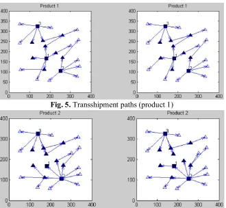
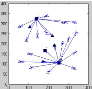
In this distribution network, five products are distributed. Since plants have limited production capacity for products, different scenarios are considered for the production capacity. All three plants have a high production capacity for product 1. Plant 1 does not produce product 2, but plants 2 and 3 have a high production capacity for this product. The only plant producing product 3 is plant 1. To produce product 4, plants 2 and 3 have a high capacity while plant 1 has a limited capacity (20% of the total demand of customers) and to produce product 5, plant 1 has a high capacity while plants 2 and 3 have a limited capacity (20% of the total demand of customers). In Fig. 5 to Fig. 9 the transshipment paths for each product before and after the local search phase are shown; the left plot represents the before local search paths, and the right plot represents the after local search paths.
Fig. 5. Transshipment paths (product 1)
Fig. 7. Transshipment paths (product 3)
Fig. 8. Transshipment paths (product 4)
Fig. 9. Transshipment paths (product 5)
Fig. 10. Result of Run 1 Fig. 11. Result of Run 2
The average CPU time of the heuristic developed by Duhamel et al. (2010) to for solve large-size two-layer LRPs, instances with 200 customers, are 965 seconds for Prodhon's instances with 10 depots and 1,255 seconds for Tuzun's instances. In addition, the average CPU time of the heuristic presented by Yu et al. (2010) to solve two-layer LRPs, instances with 200 customers and 10 depots, is 1,485 seconds. We used an Intel(R) Core(TM) i5 CPU (3.19GHz) machine with 3.17 GB of RAM to solve the problem. The computational time of the heuristic that we presented in this paper for the four-layer LRP with 3 plants, 20 CDs, 30 RDs, and 380 customers is 165 seconds, which is a very reasonable amount of time. Note that the presented four-layer LRP is a much larger and more complex problem than a two-layer LRP.
To make sure that the heuristic obtains high quality solutions, we used the heuristic to solve different versions of the sample small problem that we solved by the mixed integer programming model in Hamidi et al. (2011, 2012a). The small problem has 2 plants, 2 CDs, 2 RDs, and 4 customers. The problem was solved with different production capacities for plants. The heuristic achieved the optimal solution, verified by enumeration, for every version of the problem.
We used a confidence interval analysis to verify the reliability of the heuristic. The above large problem was solved 30 times by the heuristic. The best solution of each run is shown in Table 1.
Table 1
Best solutions
Run Best Solution Run Best Solution Run Best Solution
1 559,014 11 549,870 21 551,519
2 546,043 12 551,755 22 547,543
3 553,556 13 545,893 23 556,564
4 550,421 14 549,359 24 543,495
5 537,039 15 551,208 25 557,512
6 560,612 16 561,156 26 553,278
7 545,858 17 552,841 27 544,502
8 548,423 18 548,814 28 557,512
9 556,498 19 551,212 29 553,278
10 549,296 20 551,107 30 544,502
distribution with the mean of μ and the standard deviation of
n. The 99% confidence interval (α=0.01) for the best solution mean will be:
1 ] [ Z n XP , (4)
]1[
n Z X
P , (5)
99 . 0 ] 320 , 553 [ ] 30 478 , 5 33 . 2 989 , 550
[
P
P . (6)
This analysis shows that with the probability of 99% the best solution mean is less than or equal to 553,320. It was seen that only 33 solutions out of 3600 solutions generated in 30 runs (only 0.9% of the solutions) are less than or equal to the upper limit of the confidence interval (553,320). Note that the 3600 solutions are greedy solutions. This approves the reliability of the heuristic algorithm.
Finally, if the constraint of direct shipment distance is relaxed, the four-layer LRP will become a three-layer LRP. In the three-three-layer LRP, products can be directly shipped to any facility. Hence, the heuristic is also capable of solving the three-layer LRP. Fig. 12 shows the transshipment paths for product 2 when the three-layer LRP is solved.
Fig. 12. Three-layer LRP transshipment paths for Product 2
6. Conclusions
The LRP studied in this work is a complex multi-product four-layer capacitated LRP. This LRP is an extension of the LRP that we discussed in Hamidi et al. (2012b). In this LRP, two specific constraints are taken into account: 1) plants have limited production capacity, and 2) central depots have limited capacity for storing and transshipping products. In this paper, a heuristic algorithm is developed to solve large problems. The main components of this heuristic are a GRASP that has been developed for this particular problem and two intensification and diversification strategies that are developed to efficiently search the solution space. Results indicate that the heuristic solves the LRP effectively in terms of computational time and solution quality.
References
Aksen, D., & Altinkemer, K. (2008). A location-routing problem for the conversion to the “click-and-mortar” retailing: The static case. European Journal of Operational Research, 186(2), 554-575. Ambrosino, D., & Grazia Scutellà, M. (2005). Distribution network design: new problems and related
Ambrosino, D., Sciomachen, A., & Scutellà, M. G. (2009). A heuristic based on multi-exchange techniques for a regional fleet assignment location-routing problem. Computers & Operations Research, 36(2), 442-460.
Balakrishnan, A., Ward, J. E., & Wong, R. T. (1987). Integrated facility location and vehicle routing models: Recent work and future prospects. American Journal of Mathematical and Management Sciences, 7(1), 35-61.
Barreto, S., Ferreira, C., Paixao, J., & Santos, B. S. (2007). Using clustering analysis in a capacitated location-routing problem. European Journal of Operational Research, 179(3), 968-977.
Bruns, A., Klose, A., & Stähly, P. (2000). Restructuring of Swiss parcel delivery services. OR-Spektrum, 22(2), 285-302.
Clarke, G., & Wright, J. W. (1964). Scheduling of vehicles from a central depot to a number of delivery points. Operations research, 12(4), 568-581.
Duhamel, C., Lacomme, P., Prins, C., & Prodhon, C. (2010). A GRASP× ELS approach for the capacitated location-routing problem. Computers & Operations Research, 37(11), 1912-1923. Feo, T. A., & Resende, M. G. (1995). Greedy randomized adaptive search procedures. Journal of
global optimization, 6(2), 109-133.
Glover, F., & Laguna, M. (1997). Tabu search (Vol. 22). Boston: Kluwer academic publishers.
Hamidi, M., Farahmand, K., & Sajjadi, S. R. (2011). Modeling a Four-Layer Location-Routing Problem. In Proceedings of the 2011 IAJC-ASEE International Conference, Hartford, CT, USA. Hamidi, M., Farahmand, K., & Sajjadi, S. R. (2012a). Modeling a four-layer location-routing problem.
International Journal of Industrial Engineering Computations, 3(1), 43-52.
Hamidi, M., Farahmand, K., Sajjadi, S. R., & Nygard, K. E. (2012b). A hybrid GRASP-tabu search metaheuristic for a Four-Layer Location-Routing Problem. International Journal of Logistics Systems and Management, 12(3), 267-287.
Laporte, G. (1988). Location-routing problems, in: Golden, B. L., Assad, A. A., Vehicle Routing: Methods and Studies, North-Holland, Amsterdam. 163-198.
Larsen, R.C., & Odoni, A.R. (2007). Urban operation research: logistical and transportation planning methods (2nd edition). Dynamic Ideas Belmont, Massachusetts.
Lee, J. H., Moon, I. K., & Park, J. H. (2010). Multi-level supply chain network design with routing. International Journal of Production Research, 48(13), 3957-3976.
Lin, J. R., & Lei, H. C. (2009). Distribution systems design with two-level routing considerations. Annals of Operations Research, 172(1), 329-347.
Marinakis, Y., & Marinaki, M. (2008). A bilevel genetic algorithm for a real life location routing problem. International Journal of Logistics: Research and Applications, 11(1), 49-65.
May, M. D., & Tu, C. Y. (2008, December). Location-routing based dynamic vehicle routing problem for express pick-up service. In IEEE International Conference on Industrial Engineering and Engineering Management, 2008. IEEM 2008. (pp. 1830-1834). IEEE.
Min, H., Jayaraman, V., & Srivastava, R. (1998). Combined location-routing problems: A synthesis and future research directions. European Journal of Operational Research, 108(1), 1-15.
Nagy, G., & Salhi, S. (2007). Location-routing: Issues, models and methods. European Journal of Operational Research, 177(2), 649-672.
Prins, C., Prodhon, C., & Calvo, R. W. (2006). Solving the capacitated location-routing problem by a GRASP complemented by a learning process and a path relinking. 4OR, 4(3), 221-238.
Rego, C. (2001). Node-ejection chains for the vehicle routing problem: Sequential and parallel algorithms. Parallel Computing, 27(3), 201-222.
Resende, M. G., & Ribeiro, C. C. (2003). Greedy randomized adaptive search procedures. In Handbook of metaheuristics (pp. 219-249). Springer US.
Sajjadi, S.R., Hamidi, M., Farahmand, K., & Khiabani, V. (2011). A greedy heuristic algorithm for the capacitated location-routing problem. In Proceedings of the 2011 Industrial Engineering Research
Conference (IERC), Reno, NV, USA.
Wu, T. H., Low, C., & Bai, J. W. (2002). Heuristic solutions to multi-depot location-routing problems. Computers & Operations Research, 29(10), 1393-1415.