J.-S. Dhersin, Editor
OPTIMIZATION AND STATISTICAL METHODS FOR HIGH FREQUENCY
FINANCE
∗Marc Hoffmann
1, Mauricio Labadie
2, Charles-Albert Lehalle
3, Gilles
Pag`
es
4, Huyˆ
en Pham
5and Mathieu Rosenbaum
6Abstract. High Frequency finance has recently evolved from statistical modeling and analysis of financial data – where the initial goal was to reproduce stylized facts and develop appropriate inference tools – toward trading optimization, where an agent seeks to execute an order (or a series of orders) in a stochastic environment that may react to the trading algorithm of the agent (market impact, invoentory). This context poses new scientific challenges addressed by the minisymposium OPSTAHF.
Introduction
High Frequency Finance requires increasingly sophisticated algorithms in order to manage a series of orders from the point of view of an agent (a trader) that wishes to execute his or her orders in a limited amount of time, under various trading objectives and market constraints, possibly at very fine temporal scales. Section 1 (contributed by M. Labadie) gives a general framework for operating such a task, by means of a stochastic control program (using HJB equations) in order to deal with inventory constrainsts. Section 2 (contributed by Gilles Pag`es) proposes a new on-line optimisation algorithm for posting passive orders in a limit order book. Section 3 (contributed by H. Pham) proposes a tick-by-tick price model that incoporates microstructure effects at fine scales and that diffuses at coarse scales and for which a stochastic control algorithm for executing orders is developed. Finally, Section 4 (contributed by C.A. Lehalle) offers a wider view for order book dynamics reviewing some recent approaches and suggesting an opening in the direction of the recent and attractive mean-field game theory.
1.
HF trading under inventory and directional risk constraints
1.1.
High-frequency trading and market-makers.
The high-frequency traders (HFTs) are trading algorithms, with the fastest response or lowest latency, that buys and sells assets in electronic and listed markets, trying to capitalise ephemeral arbitrage opportunities.
∗This paper is based on the mini-symposium OPSTAHF (OPtimization and STAtistical methods for High Frequency finance)
organized by M. Hoffmann and M Rosenbaum that took place in the 2013 SMAI workshop.
1 Universit´e Paris-Dauphine and CEREMADE, CNRS UMR 7534. 2 EXQIM.
3 Capital Fund Management (CFM).
4 Universit´e Pierre et Marie Curie and LPMA, CNRS UMR 7599. 5 Universit´e Paris-Diderot and LPMA, CNRS UMR 7599. 6 Universit´e Pierre et Marie Curie and LPMA, CNRS UMR 7599.
c
EDP Sciences, SMAI 2014
One special kind of HFTs are market-makers. HFTs offer liquidity to the market, i.e. they place both a buying and a selling limit order on the Limit Order Book (LOB). Since they are offering liquidity, their buying price (bid price) is smaller than their selling price (ask price); therefore, each time they buy and sell they earn the spread (difference between ask and bid prices). However, market-makers suffer execution risks since they cannot control when and how their orders will be executed.
1.2.
Stochastic model and Hamilton-Jacobi-Bellman equation (HJB)
The optimisation programme for a market-maker is thus to maximise the profit by trading the spread over and over throughout the day whilst minimising both the execution and inventory risks. We extend the model of Avellaneda and Stoikov [3], where the only state variable is the mid-priceS(t), to a general Markovian setting with several continuous state variablesY(t) = (S(t),Σ(t), Z(t), . . .). In our case Z(t) is the half-spread of the market and Σ(t) the volatility of the mid-price. We use the convention of small letters for the values of the state variables at time t, e.g. y =Y(t). The market-maker places two limit orders of one share on each side of the LOB: a selling limit order atS(t) +δ+ and buying limit order at S(t)−δ−. The arrival of buying and selling market orders to the LOB is assumed to be Poisson and independent; the distribution of how many levels in the LOB are comsumed by a single market order is exponential (see Avellaneda and Stoikov [3] for details).
Assume the utility function is the PNL (profit and loss) X(t) +S(t)Q(t). Since the only variables the market-maker can control is where to place her quotes, i.e. (δ+, δ−), then her value function is (see Fodra and Labadie [7, 8])
u(t, y, q, x) = max
(δ+,δ−)Et,y,q,x[X(T) +Q(T)S(T)], (1)
whereEt,y[·] :=E[· |Y(t) =y]. The associated HJB equation of (1) is
(∂t+L)u+ max δ+∈AAe
−k[z+δ+]
u(t, y, q−1, x+ (s+δ+))−u(t, y, q, x)
(2)
+ max δ−∈AAe
−k[z+δ−]
u(t, y, q+ 1, x−(s−δ−))−u(t, y, q, x)
= 0,
u(T, y, q, x) = x+qs ,
where L is the infinitesimal operator associated to the continuous state variablesY(t). The jump part of the equation ( i.e. the max terms) corresponds to the infinitesimal operator for the discrete state variableQ(t). In the presence of inventory-risk aversion εand transaction costs α, the HJB equation takes the form (see Fodra and Labadie [7, 8])
(∂t+L)u+ max δ+∈AAe
−k[z+δ+]
u(t, y, q−1, x+ (s+δ+)−α)−u(t, y, q, x)
(3)
+ max δ−∈AAe
−k[z+δ−]
u(t, y, q+ 1, x−(s−δ−)−α)−u(t, y, q, x)
= ενσ2q2,
u(T, y, q, x) =x+sq − εηzq2.
1.3.
Exact solution without inventory penalty
When there is no inventory penalty, the exact solution of the HJB equation (2) is (see Fodra and Labadie [7,8])
u(t, y, q, x) = uhold(t, y, q, x) +umm(t, y), (4)
uhold := x+q(s+ ∆), ∆ :=Et,y[S(T)]−s
umm :=
2 eEt,y
" Z T
t A Ke
−KZcosh(K∆)dξ
#
,
ψ∗ := δ+∗ +δ−∗ = 2
k (market-maker’s spread),
r∗ :=
p++p−
2 =s+ ∆ (centre of spread).
From (4) we get the following observations. (i) The solutionuhas two strategies: onebuy-and-hold uhold, which is the expected value of the portfolio if the trader keeps the position until the end, and onemarket-maker umm, which is the gain from trading the spread very fast and frequently (hence the integral). (ii) Sinceumm>0, the market-maker gets a better PNL by trading the spread than a buy-and-hold investor. (iii) The market-marker’s spread ψ∗ is constant and inveresly proportional to k: whenk increases, the market orders are less likely to consume several levels of the LOB, hence the market-maker needs to offer better prices to get executed, which means a smaller spread. (iv) The centrer∗of the spread is not the current mid-pricesbutEt,y[S(T)], i.e. the conditional expectation of the value of the mid-price. This means that the market-maker plays a price arbitrage: she tilts her quotes, accepting an inventory risk, in order to capitalise the current mispricing in the long run.
1.4.
Asymptotic solution with inventory penalty
In the case of inventory penaltyεand transaction costsα, the solution and controls are not explicit. However, using perturbation methods onε we can find the explicit expresion of the controls up to first-order (see Fodra and Labadie [8]):
ψα∗ = 2
k + 2α+ 2επ˜+O ε 2
(market-maker’s spread), (5)
rα∗ = s+ ∆−ε
(
Et,y
" Z T
t
H(α)˜πdξ
#
+ 2qπ˜
)
+O ε2
(centre of spread),
∆ := Et,y[S(T)]−s ,
H(α) := 4 eAe
−K(Z+α)sinh(K∆),
˜
π := ηEt,y[Z(T)] +νEt,y
" Z T
t Σ2dξ
#
.
2.
Optimal posting price of limit orders : learning by trading
2.1.
Introduction
Our aim is to propose an on-line optimization posting method of passive orders in a limit order book, without specifying the limit order book dynamics. We consider an agent who wants to buy during a short period [0, T] a quantityQT of traded assets and we look for the optimal distance to the “fair” price (usually mid-, possibly best bid) where he has to post his limit order to minimize the execution cost (the case of a sell limit order may be obtained by symmetry). We assume the agent is alearning trader: he searches for the optimal posting distance (the price that balances adverse selection and non execution risk) by successive trials, errors and corrections. The derived recursive optimization procedure yields the best price adjustment to apply to an order for a given stopping time (reassessment dates) given past market observations.
We model the execution process of orders by a Poisson process (Nt(δ))0≤t≤T with intensity ΛT(δ, S) depending on the fair price (St)t≥0 and the distance of order submissionδ. The execution cost results from the sum of the price of the executed quantity and a penalty function depending on the remaining quantity to be executed at the end of the period [0, T]. This penaltyκΦ(Q) models the excess cost induced by crossing the spread and the resulting market impact of this execution. An optimal distanceδ∗ is defined as a minimizer of the execution cost. This leads to an optimization problem under constraints which we solve by using a recursive stochastic procedure with projection (see [14] and [15]). We prove the a.s. convergence of the constrained algorithm under additional assumptions on the execution cost function (and light assumptions on the fair price dynamics (St)t∈[0,T]). From a practical viewpoint, we give criteria on the model parameters that ensure the viability of the algorithm and the existence of a cost minimizer) relying on a functional co-monotony principle presumably satisfied by the fair price process.
2.2.
Modeling and design of the algorithm
We focus our work on the problem of optimal trading with limit buy orders on one security. We only model the execution flow which reaches the price where the limit order is posted on a short period T with a Poisson process, namely
NT(δ) with intensity ΛT(δ, S) :=
Z T
0
λ(St−(S0−δ))dt, (6)
where 0 ≤ δ ≤ δmax (δmax ∈ (0, S0) is the depth of the order book), λ : [−S0,+∞) → R+ is a finite non-increasing convex function and (St)t≥0 is a c`adl`ag stochastic process modeling the dynamics of the the best opposite price of a security stock.
Over the period [0, T], we aim to execute a portfolio of sizeQT ∈Ninvested in the asset S. The execution
cost for a distanceδisE
(S0−δ) QT∧N
(δ)
T
. We add to this execution cost amarket impact penalty function
Φ :R7→R+, non-decreasing and convex, with Φ(0) = 0, to model theimpact effect(additional cost )induced
by the execution of the remaining quantityQT−N
(δ)
T
+. The resulting cost function reads
C(δ) :=E
h
(S0−δ)
QT∧N
(δ)
T
+κ STΦ
QT −N
(δ)
T
+
i
, δ∈[0, δmax] (7)
(where κ > 0 is a free tuning parameter). Prior to solving min0≤δ≤δmaxC(δ) by implementing a stochastic
gradient descent numerically, we show that under natural assumptions on QT and κ, the function C is twice differentiable and strictly convex on [0, δmax] with C0(0) <0 and that the derivatives C(k), k= 0,1,2, have a representation as an expectation. Consequently,
The representation ofC0as an expectation means that there exists a Borel functionalH : [0, δmax]×D([0, T],R)→
Rsuch that C0(δ) =E
h
H δ,(St)t∈[0,T]
i
,δ∈[0, δmax] whereD([0, T],R)→Rdenotes the set of c`adl`ag
func-tions from [0, T] toR(see [18] for an explicit form forH). In practice to implement numerically the recursive procedure, we have to replace the “copies”S(n)by copies ¯S(n)of a time discretization ¯S= ( ¯Sti)0≤i≤m, typically
an Euler scheme of a Brownian diffusion process. Then, with an obvious abuse of notation for the functionH, we can write the implementable procedureas follows:
δn+1= Proj[0,δmax]
δn−γn+1H
δn, S¯
(n+1)
ti
0≤i≤m
, n≥0, δ0∈[0, δmax], (8)
where S¯t(in)
0≤i≤m are copies of ( ¯Sti
0≤i≤m either independent or sharing “ergodic” properties, namely some averaging properties in the sense of [19]. In the first case, one will think about simulated data after a calibration process and in the second case to a direct implementation using a historical high frequency database of best opposite prices of the asset S.
Severala.s.convergence results are established in [18] under various types of assumptions on the sequences ( ¯St(n)
i )0≤i≤m: a first setting is to assume that the ( ¯S
(n)) are i.i.d.which correspond in the real world to the
Monte Carlo simulation of a formerly calibrated model for the dynamics ofS; in a second setting we assume that we work with a historical high frequency dataset of prices of the asset assumed to share rather light averaging properties. In both cases we show that
δn a.s.
−→δ∗.
Several numerical experiments on a true dataset ar reproduced and analyzed in [18].
2.3.
Criteria for the convexity and monotony at the origin
In this section, we look for simple criteria involving the parameter κ, that imply the requested assumption on the execution cost function C (or ¯C) without never needing to really specify the process S. The original form of the criteria implying that C0(0) <0 and C00 ≥0 cannot really be used in practice since they involve ratios of expectations of functionals combining both the dynamics of the assetSand the execution parameters in a highly nonlinear way. The key establishing the criteria is thefunctional co-monotony principleestablished in [18, 29] for a wide class of diffusions and their associated time discretization schemes.
Definition 2.1 (Co-monotony). A Borel functional F : D([0, T],R) → R is non-decreasing (resp.
non-increasing) if
∀α, β∈D([0, T],R), (∀t∈[0, T], α(t)≤β(t)) =⇒F(α)≤F(β) (resp. F(α)≥F(β)).
Two functionalsF andGonD([0, T],R) are co-monotonic if they have the same monotony. A functionalF has
polynomial growth if
∃r >0 s.t. ∀α∈D([0, T],R), |F(α)| ≤K(1 +kαkr∞).
Definition 2.2 (Functional co-monotony principle). A c`adl`ag (resp. continuous) process (St)t∈[0,T] satisfies a functional co-monotony principle if for every pairF, G: D([0, T],R)→Rof co-monotonic PS-a.s. continuous Borel functionals (for the sup-norm over [0, T]) with polynomial growth such thatF(S),G(S) andF(S)G(S)∈ L1, one has
E
h
F (St)t∈[0,T]
G (St)t∈[0,T]
i
≥EhF (St)t∈[0,T]
i
E
h
G (St)t∈[0,T]
i
. (9)
Among processes satisfying such a functional monotony principle, the (fractional) Brownian motion, Brownian one-dimensional diffusions, Liouville processes L´evy processes, etc (see [29]).
Theorem 2.3. Assume that (St)t∈[0,T] satisfies a functional co-monotony principle. Assume that λ(x) = Ae−kx,x∈
(a)Monotony at the origin:
C0(0)<0 as soon as QT ≥2T λ(−S0) and κ≤
1 +kS0
kE[ST] (Φ(QT)−Φ(QT−1)) .
(b) Convexity. Let ρQ ∈
0,1−P(Nµ=Q T−1) P(Nµ≤QT−1)
|µ=T λ(−S0)
. IfΦ6= id, assume that Φsatisfies
∀x∈[1, QT −1], Φ(x)−Φ(x−1)≤ρQ(Φ(x+ 1)−Φ(x)).
If QT ≥2T λ(−S0)and κ≤
2 kE[ST] Φ0`(QT)
, thenC00(δ)≥0,δ∈[0, δmax], so thatC is convex on[0, δmax] or
for the Euler scheme of (St)t∈[0,T] with step mT, for m≥mb,σ of a diffusion with constant diffusion coefficient. (c) The same inequalities hold for tany Rm+1-time discretization sequence (Sti)0≤i≤m which satisfies a co-monotony principle.
3.
Semi Markov model for market microstructure and HF trading
3.1.
Markov renewal model for stock price
The dynamics of the mid-price are given by the c`ad-l`ag piecewise constant process:
Pt = P0+ 2δ
Nt
X
n=1 Jn,
where P0 is the opening mid-price, 2δ > 0 is the tick size,Nt is the point process associated to the tick times (Tn)n (i.e. the price jump times), and (Jn)n is the marks sequence valued in {+1,−1} indicating whether the price jumped upwards (Jn = +1) or downwards (Jn =−1) at time Tn, called price direction. We use a Markov renewal approach to model the marked point process (Tn, Jn). (Jn) is an irreducible Markov chain with symmetric transition matrix of diagonal terms 1+2α, and antidiagonal terms 1−2α, where α∈[−1,1) represents the correlation between two consecutive price returns. Estimation on real data leads to a negative value ofα, meaning that the stock price exhibits a short-term mean-reversion, which is a well-known stylized fact about high-frequency data, also called microstructure noise. Denoting bySn=Tn−Tn−1the sequence of inter-arrival times associated to (Nt), we assume that conditionally on the sign JnJn+1 = ±1 of two consecutive price directions, (Sn)nis an independent sequence with distribution: F±(s) =P[Sn+1≤s|JnJn+1=±1], and density f±(s). The distinction betweenF+andF−models the clustering of trading activity, that is the irregular spacing of tick times according to the mean-reverting or trend period of price jumps. We denote by F = 1+2αF+ +
1−α
2 F− the unconditional distribution of (Sn). The intensity function of price jump in the same (resp. opposite) direction is then given by: h+ = 1+2α1−f+F (resp. h− = 1−2α
f−
1−F).
Markov embedding. Let us define the last price jump direction: It=JNt, and the elapsed time since the last
jump: St=t−sup{Tn :Tn ≤t}. Then, the price process (Pt) is embedded into a Markov system (Pt, It, St) with three observable state variables.
Diffusive behavior at macroscopic scale. The scaled price processPt(T)= P√tT
T,t∈[0,1], exhibits a diffusive behavior given by the following functional central limit theorem:
lim T→∞P
(T) (=d) σ
∞W,
whereW is a Brownian motion, andσ2
∞ =
1
R∞ 0 tdF(t)
1+α
1−α
is the macroscopic variance. Estimation, simulation
3.2.
Market order flow modeling
We model the market order flow of the Limit Order Book (LOB) by a marked point process (θk, Zk)k, where (θk)k represents the arrival times of the market order, and (Zk)k, valued in {±1} is the side of the exchange in the LOB: Zk = +1 (resp. −1) means that the trade is exchanged at the best bid (resp. ask) price, thus associated to a market sell (resp. buy) order. The existing dependence between the market order flow and the stock price is modeled as follows. The counting process (Mt)t associated to (θk)k is a Cox process with conditional intensityλ(St), whereλ(s) is a decreasing function, representing the fact that trade arrivals should occur less often in a period of price stability, i.e. whenStis large. The dependency between market order trade and stock price is modeled through the relation: Zk = ΓkIθk−, where (Γk)k is an i.i.d. sequence on{±1} with
mean ρ∈[−1,1]. This means that ρ=Corr(Zk, Iθ−k), with the interpretation that when ρ >0 (resp ρ <0) most of the trades arrive on the strong (resp. weak) side +Iθk− (resp. −Iθk−) of the LOB. Estimation on real
data usually leads to negative value of ρ, which formalizes the observed fact that most of the trades arrive in the unfavorable side of the LOB for the market maker, inducing the so-called adverse selection risk.
3.3.
The market making application
The agent strategy consists in placing continuously limit orders of small size L at the best available price, while respecting an inventory constraint: her control is described by a process (`±t)tvalued in {0,1} with the convention that when`±t = 1, a limit order of sizeLis posted at timeton the side±It−. When a market order arrives, she is executed on the side±It−of the LOB, of`±t times a random variable distributed asϑ
±
L(dk), with support on{0, . . . , L}. The objective of the market maker is to maximize over her limit orders strategies the expected gain:
EP N LT −CLOSE(YT)−η·RISK0,T, (10)
whereP N LT =XT+YTPT is the portfolio value at terminal dateT, evaluated at the mid priceP, withX the cash holdings, andY the inventory constrained to lie in a given bounded setY,CLOSE(YT) =−(δ+ε)|YT|, is the liquidated value of the inventory at terminal date with ε≥ 0 a fixed fee paid at each transaction, and RISK0,T =
RT
0 Y 2
t ·d[P]trepresents the market risk by holding the inventory during the whole trading period, weighted by the penalization parameter η ≥0. The value functionv to this Markovian stochastic control on finite horizon (10), involving the state variables (t, Pt, It, St, Xt, Yt), can be written in the reduced-form:
v(t, p, i, s, x, y) = x+yp+ω(t, s, yi),
whereω(t, s, q) is the unique bounded viscosity solution to:
∂t+∂sω+ 2δ(h+−h−)q−4δ2η(h++h−)q2
+ max q−`L∈Y
N+
trd[`] +N
+
jmp[`]
ω+ max q+`L∈Y
Ntrd− [`] +Njmp− [`]
ω = 0,
ω(T, s, q) = −|q|(δ+ε),
and the operatorsN’s are given by:
Ntrd± [`]ω := 1±ρ 2 λ(s)
Z
[ω(t, s, q∓k`)−ω(t, s, q) +k`(+δ−ε)]ϑ±L(dk)
Njmp± [`]ω := h±(s) [ω(t,0,±q−L`)−ω(t, s, q) +L`(−δ−ε)].
solving this IODE, and illustrate our results with some computational tests displaying the shape of the optimal policies, see [27].
4.
Dynamical models for orderbook dynamics: which ones and what for
This work is mainly based on the paper Efficiency of the Price Formation Process in Presence of High Frequency Participants: a Mean Field Game analysis, a joint work with PL Lions, JM Lasry and A Lachapelle [16].
4.1.
The emergence of a need in orderbook dynamics modelling
To manage the increase of complexity following the multiplication of venues and dispersion of liquidity across all trading venues available, market participants more intensively used electronic trading and quantitative (i.e. optimal) slicing of large orders [1]. Besides, the need for cross-venue arbitrage of latency and liquidity increased, giving birth to a new kind ofmiddle-men: the High Frequency traders [26]. A better understanding of the orderbook dynamics improves: the understanding by regulators and policy makers of the contribution of each market participant to the efficiency of the PFP (Price Formation Process); the existing market impact models ( [10] [2] [21] [24]), a key component of the PFP dynamics; and the capability to use more sophisticated optimal execution schemes ( [4] [30] [13] [12]).
Recently, some papers focused on this topic: a Dynamic Model of the Limit Order Book [31]; a Fokker-Planck description for the queue dynamics of large tick stocks [9]; Price Dynamics in a Markovian Limit Order Book Market [6]; Measuring the resiliency of an electronic limit order book – [17]; State-Dependent Model of Order Book Dynamics (forthcoming, by Huang, Rosenbaum, Lehalle).
4.2.
The Mean Field Game approach as a synthesis
MFG (Mean Field Games) are designed to model this type of dynamics [20]. An MFG model of endogenous volatility has been proposed in “Large investor trading impacts on volatility” [25]. An MFG-based model has already been designed at a larger time scale in “High Frequency Simulations of an Order Book: a Two-Scales Approach” [22]. We wanted to provide a framework at the smallest one. In this paper we model participant behaviours in the orderbook; obtain “master equations” describing the emerging dynamics; use them to describe the outcome of the mixing of HFT and Institutional Investors in the same orderbook.
4.2.1. One queue modelling
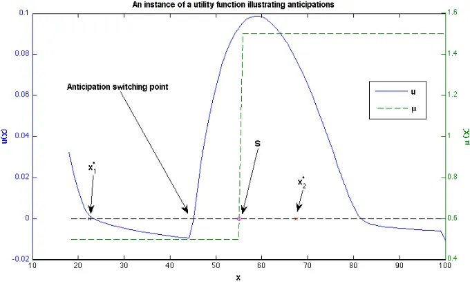
Sellers only, they arrive in the “game” according to a Poisson process of intensityλ, they compare their value functionu(x) (wherexis the size of the queue) to zero to choose to wait in the queue (whenu(x)>0) or not, the queue is consumed by a Poisson process of intensity µ(x), in case of transaction, a “pro-rata” scheme is used (“equivalent” to infinitesimal possibility to modify orders): q/xof the order is part of it; relaxed for FIFO in few slides.
Dynamics. The value function evolves following these four main possible events (we have price impactP(x) and waiting cost proportional toc q):
u(x) = (1−λ1u(x)>0dt−µ(x)dt)·u(x) ← nothing happens +λ1{u(x)>0}dt·u(x+q) ← new entrance +µ(x)dt·q
xP(x) + (1− q
x)u(x−q)
← transaction
To solve it at thekth order, we will perform a Taylor expansion ofu(x+q) andu(x−q) for smallq at the kth order). At the second order, we obtain:
0 = µ(x)
x (P(x)−u)−c+ (λ1{u>0}−µ(x))u 0+q1
2(λ1{u>0}−µ(x))u
00+µ(x)
x u
0.
This corresponds to a (trivial) shared risk Mean Field Game monotone system with N = 1. The mean field
aspect does not come from the continuum of agents (for every instant, the number of players is finite), but rather from the stochastic continuous structure of entries and exits of players.
Solution for a specific form ofµ(x). At queue sizesx∗such thatx∗=µ(x∗)P(x∗)/c,usign changes. Moreover, for the specific caseµ(x) =µ11x<S+µ21x≥S : There is a point strictly beforeSwhereuswitches from negative to positive. It means that participants anticipate service improvement.
Figure 1. All the components of the one queue model.
4.2.2. Going further
In the paper [16], a model with two coupled queues is developed and analysis in a first step, and then extended to more than one class of trading agents. We then use this model to understand the mechanism of liquidity dynamics in a limit orderbook when traditional investors are mixed with high frequency traders. Such results can help regulators and policy makers to understand the stakes and the potential consequences of their decisions to adjust the market microstructure (see [23] for more details about practical aspects).
References
[1] R. F. Almgren and N. Chriss. Optimal execution of portfolio transactions.Journal of Risk, 3(2):5–39, 2000.
[2] Robert Almgren, Chee Thum, Emmanuel Hauptmann, and Hong Li. Direct Estimation of Equity Market Impact.Risk, 18:57– 62, July 2005.
[3] Avellaneda and Stoikov. High-frequency trading in a limit-order book.Quantitative Finance, 8(3):227–224, 2008.
[4] Bruno Bouchard, Ngoc-Minh Dang, and Charles-Albert Lehalle. Optimal control of trading algorithms: a general impulse control approach.SIAM J. Financial Mathematics, 2(1):404–438, 2011.
[6] Rama Cont and Adrien De Larrard. Price Dynamics in a Markovian Limit Order Book Market. Social Science Research Network Working Paper Series, January 2011.
[7] Fodra and Labadie. High-frequency market-making with inventory constraints and directional bets.Preprint ArXiv, 2012. [8] Fodra and Labadie. High-frequency market-making for multi-dimensional markov processes.Preprint ArXiv, 2013.
[9] A. Gareche, G. Disdier, J. Kockelkoren, and J. P. Bouchaud. A Fokker-Planck description for the queue dynamics of large tick stocks, April 2013.
[10] Jim Gatheral. No-dynamic-arbitrage and market impact.Quantitative Finance, 10(7):749–759, 2010.
[11] Gu´eant, Lehalle, and Fern´andez-Tapia. Dealing with the inventory risk. a solution to the market making problem.Math Finan Econ, 7(4):477–507, 2013.
[12] Olivier Gu´eant, Charles-Albert Lehalle, and Joaquin Fernandez-Tapia. Dealing with the inventory risk: a solution to the market making problem.Mathematics and Financial Economics, September 2012.
[13] Idris Kharroubi and Huyen Pham. Optimal portfolio liquidation with execution cost and risk. June 2009.
[14] H. J. Kushner and D. S. Clark.Stochastic approximation methods for constrained and unconstrained systems, volume 26 of Applied Mathematical Sciences. Springer-Verlag, New York, 1978.
[15] H. J. Kushner and G. G. Yin.Stochastic approximation and recursive algorithms and applications, volume 35 ofApplications of Mathematics (New York). Springer-Verlag, New York, second edition, 2003. Stochastic Modelling and Applied Probability. [16] Aim´e Lachapelle, Jean-Michel Lasry, Charles-Albert Lehalle, and Pierre-Louis Lions. Efficiency of the Price Formation Process
in Presence of High Frequency Participants: a Mean Field Game analysis, May 2013.
[17] Jeremy Large. Measuring the resiliency of an electronic limit order book.Journal of Financial Markets, 10(1):1–25, February 2007.
[18] S. Laruelle, C.-A. Lehalle, and G. Pag`es. Optimal posting price of limit orders: learning by trading. Math. and Fin. Econ., 7(3):359–403, 2013.
[19] S. Laruelle and G. Pag`es. Stochastic approximation with averaging innovation applied to finance.Monte Carlo Methods Appl., 18(1):1–51, 2012.
[20] Jean-Michel Lasry and Pierre-Louis Lions. Mean field games.Japanese Journal of Mathematics, 2(1):229–260, March 2007. [21] Charles-Albert Lehalle and Ngoc M. Dang. Rigorous post-trade market impact measurement and the price formation process.
Liquidity Guide, 2010.
[22] Charles-Albert Lehalle, Olivier Gu´eant, and Julien Razafinimanana. High Frequency Simulations of an Order Book: a Two-Scales Approach. In F. Abergel, B. K. Chakrabarti, A. Chakraborti, and M. Mitra, editors, Econophysics of Order-Driven Markets, New Economic Windows. Springer, 2010.
[23] Charles-Albert Lehalle, Sophie Laruelle, Romain Burgot, St´ephanie Pelin, and Matthieu Lasnier.Market Microstructure in Practice. World Scientific publishing, 2013.
[24] F. Lillo, J. D. Farmer, and R. Mantegna. Econophysics - Master Curve for Price - Impact Function.Nature, (421), January 2003.
[25] Pierre L. Lions and Jean M. Lasry. Large investor trading impacts on volatility.Ann. I. H. Poincar´e, December 2006. [26] Albert J. Menkveld. High Frequency Trading and The New-Market Makers.Social Science Research Network Working Paper
Series, December 2010.
[27] Fodra P. and H. Pham. High frequency trading in a markov renewal model.Preprint ArXiv, 2013. [28] Fodra P. and H. Pham. Semi-markov model for market microstructure.arXiv:1305.0105., 2013.
[29] G. Pag`es. A functional co-monotony principle with an application to peacoks and barrier options. 2012. pr´e-pub PMA 1536, to appear inS´eminaire de Probabilit´es XLV.
[30] Gilles Pag`es, Sophie Laruelle, and Charles-Albert Lehalle. Optimal split of orders across liquidity pools: a stochatic algorithm approach.SIAM Journal on Financial Mathematics, 2:1042–1076, 2011.